TRUE OPERATION SIMULATION FOR
URBAN RAIL
Energy efficiency from access to Big data
JESPER KUMLIN
School of Business, Society and Engineering
Course: Degree Project in Industrial Engineering
and Management with Specialization in Energy Engineering
Course code: ERA402 Credits: 30 hp
Program: Master of Science program in
Supervisor: Maher Azaza Examiner: Erik Dahlquist
Customer: Ganesh Chandramouli, Bombardier
Transportation
Date: 2019-06-13
ABSTRACT
New 5G mobile communication technology promises new possibilities for current and future urban railways by enabling Big data transmission. This degree project analyzes how access to true operation data can improve future and existing urban railways energy efficiency.
Discussions on which type of sensor data are interesting for urban rail traction energy
efficiency at train manufacturer Bombardier Transportation were the basis to help determine the outline of this degree project. A literature study was conducted with the focus to better understand measures to reduce energy consumption in urban rail as well as help describe challenges in their possible implementation. The method was to test how energy and
performance calculations can improve from access to true operation data. A model based on real performance data was emulated in a simulation tool and compared to models that did not have real data adaptation. The results showed the adapted model simulate energy performance very similar to the real performance data, indicating a benefit of implementing such data to create better urban railway energy and performance simulations. Access to urban railway operation data also enabled an analysis of the driving style, which could help rail operators drive more energy-efficiently. This degree project also showed better
maintenance strategies would be possible with more data access. A preventive maintenance strategy where faulty parts are changed when needed, instead of after an estimated service distance or duration has passed could lead to better energy efficiency and financial savings.
Keywords: 5G, urban rail, Big data, energy efficiency, driver advisory system, preventive
FÖRORD
Denna masteruppsats är ett examensarbete för Civilingenjörsprogrammet i industriell
ekonomi vid Mälardalens Högskola i Västerås. Examensarbetet utfördes under våren 2019 på uppdrag av Bombardier Transportation i Västerås. Jag vill tacka Ganesh Chandramouli vid Bombardier Transportation för att du ställt upp som extern handledare samt bidragit med tankar och idéer. Tack till Peder Flykt vid Bombardier Transportation för stöd kring de simuleringar som genomfördes. Även ett tack till Daniel Lag vid Bombardier Transportation för ditt mentorskap och för att du möjliggjorde detta examensarbete. Tack till Maher Azaza som varit min handledare vid Mälardalens Högskola och väglett mig genom examensarbetet. Till sist vill jag också tacka min familj, speciellt Peter Kumlin och Pontus Kumlin för
intressanta diskussioner och för att ni alltid hjälper mig att tänka utanför ramarna. Ett speciellt tack till min sambo Louise Kjell för att du alltid tar fram det bästa ur mig och hjälper mig att sikta högre.
Västerås i juni 2019 Jesper Kumlin
SAMMANFATTNING
I takt med att städer fortsätter växa ökar behovet av klimatsmarta transportsätt.
Tunnelbanor och bussar är de vanligaste transportmedlen för stadsbor. Båda förväntas växa för att klara av det ökade behovet. Men tunnelbanan anses vara mer miljövänlig på grund av att den inte använder fossila bränslen. Ett ökat antal passagerare och introduceringen av elektriskt drivna bussar ökar pressen på nuvarande tunnelbanesystem i världen. Därför är det viktigt att skapa resurseffektiv expansion och energieffektivitetsförbättringar av befintlig järnväg. Ny 5G mobilkommunikationsteknik skapar nya möjligheter för nuvarande och framtida tunnelbanor genom att möjliggöra dataöverföring i större kapacitet än tidigare. Detta examensarbete analyserar hur tillgången av verkliga driftsdata kan förbättra framtida och befintliga tunnelbanors energieffektivitet.
Metoden som använts var att testa hur energi- och prestationsberäkningar kan förbättras från tillgång till verkliga driftsdata. En modell baserad på verkliga resultatdata skapades i ett simuleringsverktyg och jämfördes med modeller som inte har den verkliga
dataanpassningen. Resultaten visade att den anpassade modellen var mycket lik den verkliga körningen, vilket indikerar en fördel med att implementera sådan data för att skapa bättre energi och prestationssimuleringar. Det visade också potentiella fördelar för tågoperatörer när körstilen kan analyseras från åtkomst till tågdriftsdata. Tillgång till mer data kan därför förväntas förbättra tågens energi och prestationssimuleringar i stadsmiljö. Detta
examensarbete visade också att bättre underhållsstrategier skulle vara möjliga med mer dataåtkomst. En underhållsstrategi där felaktiga delar byts när det behövs, till skillnad från när en förväntad livslängd har gått eller när de går sönder kan leda till stora besparingar för både energikonsumtionen och ekonomiskt.
Nyckelord: 5G, tunnelbana, Big data, energi-effektivitet, Driver advisory system, proakivt
CONTENT
1 INTRODUCTION ...1
1.1 Background ... 2
1.1.1 Railway introduction ... 2
1.1.2 Urban rail emissions... 3
1.1.3 Bombardier Transportation... 3 1.2 Problem formulation... 4 1.3 Purpose/Aim ... 4 1.4 Research questions ... 4 1.5 Delimitation ... 4 2 METHOD ...5 2.1 Data collection ... 5 3 LITERATURE STUDY ...6
3.1 Urban rail traction energy flow ... 6
3.1.1 Braking Energy ... 6
3.1.2 Traction Losses ... 7
3.1.3 Motion Resistance ... 7
3.1.4 Auxiliary Load ... 8
3.2 Urban railway digitalization ... 8
3.2.1 Maintenance 4.0 ... 9
3.2.2 Flexible adaptation of the transport capacity ...11
4 CURRENT STUDY ... 12
4.1 Degree project outline ...12
4.2 Reference case ...13
4.3 TEP ...15
4.3.1 Test conditions ...15
4.3.1.1. TRAIN SET DEFINITION ... 15
4.3.1.2. TRAIN UNIT DEFINITION ... 16
4.3.1.4. LINE FILTER INDUCTOR ... 17
4.3.1.5. EFFORT DEFINITION ... 18
4.3.1.6. TRACK AND ENVIRONMENT... 19
4.3.1.7. SCHEDULE ... 19
4.3.1.8. CONTROL SETTINGS ... 19
4.3.2 Simulations and calculations ...20
4.3.2.1. CASE 1: “ALL-OUT” ... 20
4.3.2.2. CASE 2: DAS ... 20
4.3.2.3. CASE 3: TRUE OPERATION ... 20
4.4 Maintenance data ...22
5 RESULTS ... 24
5.1 Case 1: “All-out” ...24
5.2 Case 2: DAS ...26
5.3 Case 3: True operation ...28
5.4 Energy result comparison ...30
6 DISCUSSION... 31
6.1 Urban railway energy efficiency and digitalization ...31
6.2 Better energy and performance simulations ...32
6.3 Other energy optimization implementations ...33
7 CONCLUSIONS ... 35
8 SUGGESTIONS FOR FURTHER WORK ... 36
LIST OF FIGURES
Figure 1 Typical traction energy flow in urban rail systems ... 6
Figure 2 Common maintenance strategies ... 10
Figure 3 Reference case, route one speed profile ...14
Figure 4 Reference case, route two speed profile ... 15
Figure 5 Train set definition ...16
Figure 6 Train unit definition ... 17
Figure 7 Motor settings ... 17
Figure 8 Line filter inductor properties ... 18
Figure 9 Effort definition, total braking ... 18
Figure 10 Effort definition, electrical braking ... 18
Figure 11 Effort definition, traction...19
Figure 12 Typical speed profile in TEP ...21
Figure 13 Case 1:1 Speed profile comparison ... 24
Figure 14 Case 1:2 Speed profile comparison ... 25
Figure 15 Case 2:1 Speed profile ... 26
Figure 16 Case 2:2 Speed profile ... 27
Figure 17 Case 3:1 Speed profile comparison ... 28
Figure 18 Case 3:2 Speed profile comparison ... 29
LIST OF TABLES
Table 1 Reference case data ...14Table 2 Coasting set-up ...21
Table 3 Case three top speed set-up ... 22
Table 4 Maintenance scheme ... 23
Table 5 Case 1:1 Energy results ... 24
Table 6 Case 1:2 Energy results ... 25
Table 7 Case 2:1 Energy results ... 26
Table 8 Case 2:2 Energy results ... 27
Table 9 Case 3:1 Energy results ... 28
Table 10 Case 3:2 Energy results ... 29
ABBREVIATIONS
Abbreviation DescriptionACM Auxiliary Converter Module
ATO Automatic Train Operation
BC Battery Charger
CO Carbon monoxide
DAS Driver Advisory System
DC Direct Current
EDLC Electrochemical Double Layer Capacitor
ESS Energy Storage System
kWh Kilowatt-hour
MCM Motor Converter Module
NOx Nitrogen Oxide
PM Particulate Matter
PMSM Permanent Magnet Synchronous Motor
RB Regenerative Braking
TEP Train Energy and Performance calculations
VAC Volts Alternating Current
VDC Volts Direct Current
DEFINITIONS
Definition Description
5G 5th generation cellular mobile communications Big data Large and complex data sets difficult to
work with standard software
Train A form of transport consisting of a series of connected vehicles that runs along a rail track
1
INTRODUCTION
Urban cities are home to 55.3 % or 4.26 billion of the world’s population in 2018. The UN predicts that number to rise to 60 % by 2030 (UN, 2018). With the expected continued growth of the world’s population, 5.1 billion people could be living in cities by 2030 (UN, 2019). The UN has a goal to make cities and human settlements inclusive, safe, resilient and sustainable (UN, 2018). Growing cities will put pressure on current transport modes due to the increasing number of passengers. According to Mulley, Hensher & Cosgrove (2017) the main transport modes in cities are urban railways and buses and substantial investments are required in both to ensure future generations to travel inside cities in a safe and
environmentally friendly way. More traffic will result in larger energy consumption and capacity problems for current urban railways and an increasing number of electric buses will compete with urban railways for electricity demand. Therefore, one of the most important steps is energy-efficient expansion where reducing energy consumption in urban rail systems is a key contributor.
The four major energy consumption parts in urban rail systems are traction, lighting, air-conditioning, and elevators. Research by Su, Tang & Wang (2016) and González-Gil, Palacin, Batty & Powell (2014) shows that traction energy use is between 40-80 % of the total energy needed for the whole system. They state traction energy consumption must be considered in order to achieve urban rail energy efficiency. There are today many sensors measuring temperatures, voltages, and currents (true operation data) in urban railways. This type of sensor data mainly varies by 5Vs. They are volume, velocity, variety, value, and veracity. The volume considers the magnitude of data, which is always increasing. The velocity includes how to deal with the continuously generated data at high speeds. The variety deals with the fact that data are in different formats. For example, structured or unstructured data. The value of the data is when something useful can be interpreted from it. The veracity refers to biases, noise, and abnormality in data, which can lead to inaccuracies. These factors lead to data sets with sizes current software tools cannot handle within a reasonable timeframe, also called Big data (Grover, Chiang, Liang & Zhang, 2018).
Because of Big data characteristics and security risks, not all the data is remotely accessible. The next generation of mobile communication called 5G and it promises new possibilities for the rail industry. Compared to current technology, 5G networks can handle large amounts of data in a secure way (Yang et al, 2015). Because 5G technology is not widely implemented in technical applications, not a lot of research exists on what potential benefits it may have on urban rail systems.
1.1 Background
Regarding urban railway operation optimization, there are several different fields of interest. This section will start by introducing railways.
1.1.1 Railway introduction
There are three main types of traction used in railways throughout history. They are steam-, diesel- and electrical-powered. In the mid-1940s, diesel-powered trains took over from steam-powered trains partly due to low oil prices at the time and faster fueling times. Electrically powered trains developed throughout the 1900s and have significantly higher efficiency at 65-80 % compared to 20-25 % for diesel-powered trains (Östlund, 2011). Despite higher efficiency, electrical trains only make up 30 % of the global rail fleet (Ghavia, 2018). Electrically powered trains have less greenhouse gas emissions (GHG) than diesel-powered trains, assuming the electricity is from a renewable source. Compared to other means of transport it also has a lower environmental impact, but there is room for improvement (European Commission, 2017). Electric trains are preferable in cities because of the absence of exhaust gases and its silent operation. Some of the different types of railway systems in urban rail are tramways, light rail systems, metro, and commuter railways. Railway energy consumption can be divided into traction and non-traction consumption. Traction energy is energy with the purpose of moving the train forward, as well as the onboard auxiliary system, which for instance handles the climate control. Non-traction energy consumption includes the energy used at stations and other subsystems. It contains the signaling, lighting, ventilation and groundwater pumps required to enable a functioning railway system (González-Gil et al, 2014).
Electrically powered trains exist mainly in Europe and Japan. 95 % of Sweden’s trains are electrically powered, consuming 2 % of Sweden’s total annual electrical energy produced. The advantages of electric trains over diesel-powered are where traffic density is high and high output is preferable, making them ideal for urban use (Östlund, 2011). A reason electrical trains are not widely established is the high financial cost of implementation. One kilometer of the electrified railway can cost around one million Euros to install, not counting the high continuous maintenance costs (Ghavia, 2018). Every country also has its own standards of signaling systems as well as different physical and legal requirements of the trains (Östlund, 2011). There are also many different standards of voltages in different countries because of historical circumstances. A global standard does not exist because of the high costs of
replacing existing systems and a lack of research showing the potential benefit of one system over the other, just in Europe there are five different power supply systems.
Some of the parameters are the use of direct current (DC) and alternating current (AC), as well as frequency and voltage. Trains can travel over different technology borders if they are equipped with converters, modern converters can handle up to four different input voltages. The converters can either switch from AC to DC or vice versa, step-up or step-down the voltages as well as change frequency (Östlund, 2011).
Electric trains get power from overhead contact lines. The lines could either supply power or gain power from Regenerative Braking (RB) systems. RB is defined as the process of
transforming the braking energy of trains during the deceleration into electrical energy by using the electric motors as an electric generator instead. Another option is to use energy storage systems onboard the trains. The most common versions work both with overhead power lines and independently. One main factor is that they can replace diesel-powered trains on non-electrified lines. The type of energy storage system is usually supercapacitor, battery or fuel cells (Ghavia, 2018). The benefits of using energy storage directly on the trains are increasing the range to areas where the overhead power lines do not exist, or through city centers where such power lines might be forbidden. They are also typically cheaper than constructing new infrastructure for the power lines. Some downsides are the physical space they take up on the trains and the added weight, which might limit the added advantage of better RB power utilization. Because onboard energy storage systems are difficult to
implement on current trains another option is to place them along the tracks, although that adds line losses.
1.1.2 Urban rail emissions
Even though urban rail lacks a combustion engine on-board, they have substantial emissions. Abbasi, Jansson, Sellgren & Olofsson (2013) reviewed recent research on rail particle
emissions. They highlighted the lack of regulation on non-exhaust emissions, originating from friction between wheel and rail and braking processes. They found non-exhaust particle emissions to have toxic effects, which together with high concentration levels in subway systems make it an important optimization problem. Non-exhaust emissions are affected primarily by increased axle load, train speed, but also with an increased train frequency. Therefore, they need to be considered when optimizing railway emissions. Electric rail transport has exhaust emissions mainly from maintenance vehicles. Exhaust emissions are mainly present in diesel-locomotives, but it still has lower emissions of CO, NOx, and PM than those from the road transport, aviation, and shipping sectors (Fuglestvedt et al, 2008; Uherek et al, 2010).
1.1.3 Bombardier Transportation
Bombardier Transportation is a global mobility solution provider with products and services ranging from the manufacturing of trains to the development of related sub-systems. This degree project was conducted on behalf of Bombardier transportation as a part of their interest in the development of new 5G technology and how access to true operation Big data could benefit rail operation. Big data has the possibility to help increase energy efficiency in rail systems while also leading to economic savings. Therefore, it is an interesting subject to study further.
1.2 Problem formulation
Even though studies have been made on Big data in a railway context, not a lot has been done on how access to true operation data can improve energy efficiency. This degree project analyzes interesting energy efficiency implementations from access to propulsion system sensor data in urban railways.
1.3 Purpose/Aim
Investigate how access to propulsion system sensor data can be used to improve energy efficiency in urban railways.
1.4 Research questions
- If true operation data were more accessible, which energy saving measures are possible?
- How does access to propulsion data affect energy consumption in Train Energy and Performance simulations?
1.5 Delimitation
This degree project will delimit from emission optimization and focus on the traction energy optimization of urban railways, running on 750 V DC lines. Also, the technical
implementation of 5G in the railway industry is outside the scope of this degree project. No economic calculations will be performed.
2
METHOD
To answer the research questions, an energy technical simulation was conducted. The program used was Train Energy and Performance calculations (TEP), developed by
Bombardier Transportation. Specific data required for simulations on three selected driving style cases was provided by Bombardier Transportation and used in TEP to simulate actual train performance. The simulated data were compared to actual performance data from a real test made by Bombardier Transportation to verify its authenticity. That test will be called the reference case in this degree project. The first case is called “all-out” driving, where the fastest way of completing a track is simulated. The second case use the built-in Driver Advisory System (DAS) in TEP to simulate the most energy efficient driving style. The third case aims to emulate how TEP could use sensor data on the speed profile to create a digital twin of the reference case. These three cases were selected as they represent three extreme driving styles. The first is the worst-case scenario from an energy efficiency point of view, and the second case is the best-case scenario. The third case can show how far from the other two cases TEP are when the reference case is emulated. It can also show if such implementation of sensor data to TEP is beneficial when studying the driving style of trains.
2.1 Data collection
Since there are several energy consuming processes in the propulsion of trains, people from different engineering units of Bombardier Transportation were interviewed. The units included product management, advanced engineering, system engineering, converter
engineering, drives, and Train Control & Management System. They were asked to give their view on what additional data might benefit them in their respective field of works. Their answers were the basis to help determine the outline of this degree project. Train propulsion data was also gathered from Bombardier Transportation. Specifically, data from the reference case speed profile and physical properties as well as information of track and environment was provided by Bombardier Transportation. Data from a maintenance scheme at
Bombardier Transportation was also provided to enable a discussion of preventive maintenance implementation from access to such data.
A literature study on train energy flow was conducted using Google Scholar and searching for relevant literature. Some of the keywords when searching were: 5G, urban rail, Big data, energy efficiency, driver advisory system, and predictive maintenance. The literature study was designed to add more knowledge about the different energy consuming areas, as well as help to describe challenges in their possible implementation. Therefore, both older and newer sources were relevant. Focus was also on finding methods on how to increase energy efficiency regarding traction energy in urban rail, in order to know which type of sensor data is interesting to study further.
3
LITERATURE STUDY
To answer the research questions this section investigates the different energy consuming parts in urban rail traction energy and how others have optimized the energy consumption. Then the railway digitalization is examined.
3.1 Urban rail traction energy flow
Figure 1 shows a typical traction energy flow in urban rail systems. It consists of 4 main categories: Braking energy, Motion resistance, Traction losses, and Auxiliary load. The following section reviews the different methods for energy efficiency for each category.
Figure 1 Typical traction energy flow in urban rail systems
3.1.1 Braking Energy
Braking energy stands for 50% of the net traction energy demand and with RB 33% can be recovered in a typical urban rail system, as can be seen in Figure 1. RB is especially effective in urban rail systems because of the numerous and frequent number of stops. For RB to be effective it also requires short distances between either another train to receive the energy produced or stations to send the energy back to the electricity grid (Östlund, 2011). As shown in Figure 1, RB can help to decrease the overall energy consumption for urban rail trains. Generally, the braking energy accounts for half of the total energy losses of the trains and increasing with a higher number of stops (González-Gil et al, 2014).
Yang et al (2015) considered timetable optimization and energy-efficient driving as two of the most important factors regarding railway braking energy optimization. One way of
implementing them is with the use of DAS or automatic train operation (ATO). ATO is like a DAS but instead of just giving instructions it drives the train without a human driver.
Research by Ghavia (2018) has shown a potential 28 % increase in energy efficiency with the use of a DAS. Scheepmaker, Goverde & Kroon (2017) reviewed recent research on
energy-efficient train control. They found the algorithms in current DAS and ATO systems to require some simplifications to be able to perform their calculations in real-time due to many
calculations needed.
Another option to optimize the regenerated braking energy is to use it together with energy storage. Low utilized railways limit the efficiency of RB because the energy is dissipated in the braking resistors instead of sending it to a receiving train. The inclusion of energy storage system (ESS) can increase efficiency with current RB technology by minimizing wasted energy (Ghavia, 2018). Kılıçkıran et al (2017) found that the total energy consumption of trains can be reduced from between 10 % and 45 % with the use of RB, where the higher number corresponds to less wasted energy. The most common technologies used for ESSs in urban rail are electrochemical double layer capacitors (EDLCs), batteries and flywheels. EDLCs is the most suitable for use in urban rail because of its high-power density, fast response, high cycle efficiency and long lifecycle (González-Gil et al, 2014). The regenerated energy could also be used by the trains own auxiliary systems.
3.1.2 Traction Losses
Traction losses are the energy losses from inefficiencies in power converters, electric motors, and transmission system, where losses in the power converters and transmission system can be considered as minor. The main area of improvement regarding traction losses is the electric motor. The efficiency is highly dependent on the speed and power ranges (González-Gil et al, 2014). Using too big motors adds weight and power consumption without any added benefits. While using too small motors can lead to increased wear due to the motor being pushed to its limits more often. It also increases the risk of motor failures. The key to limiting traction losses is to use the right size motor for each individual rail system.
González-Gil et al (2014) also study the type of motor, where Permanent Magnet
Synchronous Motor (PMSM) have shown a traction energy saving of between 9-13%. Partly due to its high efficiency of 97%. It does not require as much cooling leading to lighter constructions but is limited by higher investment costs. Türker, Buyukkeles & Faruk Bakan (2016) have done research on a current controller for PMSM drives. They mean it is
necessary to have a robust control scheme to prevent one of the biggest drawbacks of PMSM motor systems, torque ripples. Torque ripples create unstable systems with a higher risk of failures because there is a direct relation between the phase currents and the output torque in PMSM systems.
3.1.3 Motion Resistance
Motion resistance is the aerodynamic resistance to vehicle progression and the mechanical friction between wheels and rails. Aerodynamic resistance gets more important with increasing speeds since aerodynamic drag increases with the square of velocity. At lower speeds, mechanical resistance is more significant because it is the mass of the train that mainly affects how big it is. Higher total weight means bigger mechanical friction and more energy needed to overcome it (González-Gil et al, 2014). Due to the relatively low speeds of
urban railways the size of the motion resistance is mainly determined by the train mass. A study by Su et al (2017) showed an increase in train mass by 50% increased the energy consumption by 100%. Therefore, reducing train mass is one of the most efficient ways to lower energy consumption, especially for urban rail cars.
3.1.4 Auxiliary Load
An energy consuming part not connected to the driving force is the auxiliary load. The
auxiliary system mainly consists of onboard ventilation, air-conditioning, and lighting (Yang, et al, 2015). Therefore, it is highly dependent on climate as hot places require more cooling and colder places more warming. The difference can be exemplified by the different climates of Oslo and London. Where Metro Oslo has a 28% share of the total traction energy from the heating systems alone, and London Underground is estimated to need just 10% for all their auxiliary systems (González-Gil et al, 2014). To reduce auxiliary energy consumption, adaptive air-conditioning could be implemented. Especially effective in cold climates where on some days the auxiliary energy requirement can be greater than the traction energy. Thermal isolation of the vehicles, windows and limiting the number of door openings are effective measures but the system also needs to know the required level of air-conditioning at any given moment to be as effective as possible. Research has shown a potential energy consumption decrease of 11 % when controlling air-conditioning level to the actual temperature and CO2 concentration, by adapting air-conditioning to when it is necessary (Gunselmann, 2005).
3.2 Urban railway digitalization
Urban railway digitalization is characterized by Big data measured from sensors on railway systems. The potential access to more information on urban railway operation is an
interesting subject for researchers. Even though Big data is a new concept, there have been studies on the implementation of Big data in a railway context. Dutch railways carried out adaptive and self-learning maintenance actions from Axle Box Acceleration measurements with one terabyte of track degradation data (Núñez, Hendriks, Li, De Schutter & Dollevoet, 2014). Big data was applied in a public transport context in Utrecht, Netherlands. They wanted to handle the traffic and explain the usage of mobile phones, smart cards, and computers to predict the traffic to make operation improvements (van Oort, 2014). Hodge, O’Keefe, Weeks & Moulds (2014) examined wireless sensors network technology for
monitoring and analyzing railway systems. They highlighted the importance to validate and filter Big data from errors to create useful information flows. Turner, Tiwari, Starr & Blacktop (2015) studied railway-related planning and scheduling issues. They also concluded that the ability to interpret Big data is a key focus for future knowledge-based and autonomous rail systems.
To be able to use Big data, a new way of handling and sending the data is required. The next generation of mobile communication is called 5G and it promises new possibilities for the rail industry. Current research shows 5G networks to be able to handle larger amounts of data
with better reliability, compared to current technology (Yang et al, 2015). It enables the introduction of smart systems to increase energy efficiency and stability. Intelligent cyber-physical systems are integrated into devices for monitoring and control purposes. These systems are connected and communicate with each other through internet technology, enabling remote access to data. It can also help predict failures, makes a diagnosis and triggers maintenance actions (Kans & Ingwald, 2016).
Increased wireless communication also increases the risk of cyber-attacks. One important reason for the limitations of wireless information flow from urban railways today is the security risk. Cyber-espionage to gain illegal access to sensitive information about the trains or cyberterrorism to hi-jack the trains operating system to cause damage to infrastructure or people (Gomes et al, 2018). The implementation of 5G technology could be a key factor in solving the problem of cyber-security risks. The emergence of 5G networks will offer two major advantages over current security techniques. Instead of trying to stop hackers by adding complex computational obstacles, physical layer security limits the physical transmission itself from being accessible to unauthorized people. Physical layer security techniques also have more scalability, making it ideal for growing networks (Yang, et al, 2015; Wu, et al 2018).
3.2.1 Maintenance 4.0
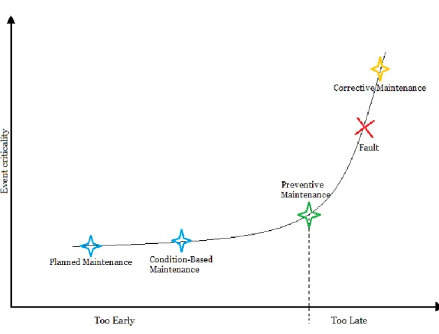
Hitachi (2018) have been looking at how predictive maintenance could be implemented in the rail industry. They state that there are four main maintenance strategies in railway operation. Planned maintenance is a service of parts after a certain time plan. Condition-based maintenance instead uses a set amount to determine when maintenance is required. It can be how many miles a train has rolled or how many revolutions a fan has turned. Both methods are usually set with a margin towards the safer side to not risk failure of
components. Corrective maintenance is maintenance on damaged parts. Parts which have already experienced failure and often caused unplanned stops. This means that corrective maintenance is the most expensive form of maintenance. Preventive maintenance means measuring critical components and find patterns of when the components need maintenance. Figure 2 shows how the maintenance strategies relate to each other with respect to time.
Figure 2 Common maintenance strategies
Kans, Galar & Thaduri (2016) explored the possible advantages of implementing smart systems connected to the internet to improve railway maintenance systems, also called Maintenance 4.0. These smart systems could connect trains to a network and be easily monitored in a way not previously possible due to the large data volumes required. They could also predict failure, make diagnostics and trigger maintenance actions. However, these systems require high data quality as well as good data access (Lee, Kao & Yang, 2014). If such data were available, maintenance 4.0 could enable scalable and upgradable systems, utilizing standardized products and interfaces. This would enable easy migration from legacy systems, which is key in the creation of new railway systems due to new trains often runs together with older trains.
Kans et al (2016) conclude that maintenance 4.0 would improve the energy efficiency and sustainability of the systems. Maintenance 4.0 systems could maximize capacity and utilization of the trains minimizing shutdowns, and therefore increasing energy efficiency. The high installation costs together with the many different types of systems requiring complex integration for example in the European rail network might limit the rail industry growth. Therefore, reducing operation and maintenance costs while keeping a high level of security is key to enable a growing rail industry (European Commission, 2017).
3.2.2 Flexible adaptation of the transport capacity
The concept of flexible capacity adaptation is to better match actual passenger loads with available capacity so as not to haul empty train cars. Operating trains with respect to its maximum capacity needs all the time leads to massive unnecessary energy consumption due to passenger fluctuations during the day. The problem is how to accurately anticipate what the capacity need will be at any given station and time of day. As well as to have a flexible system to quickly change the number of cars (Gunselmann, 2005). Frumin (2010) studied methods to measure passenger loads on trains from a historical data set. He found weight measurements from sensors in train suspension systems to be the most accurate on individual trains, compared to passenger volume data from the station's electronic gates. Sugiyama et al (2010) examined an approach for real-time estimation of railway passenger flow. They preferred to use the station electronic gates data due to the large data volumes required. Therefore, to implement real-time passenger flow information from train suspension sensor data the system must be able to send, receive and handle large data volumes.
4
CURRENT STUDY
This section starts by summarizing the discussions with people at Bombardier
Transportation, which were the outline for this degree project. Then the reference case, which was the basis for the three cases in TEP is presented. Then the input data for TEP simulations are explained. This section ends with an actual maintenance scheme from Bombardier
Transportation to provide a basis for a discussion on other possible benefits from access to more sensor data.
4.1 Degree project outline
Discussions at Bombardier Transportation showed several benefits and challenges with different types of potential data collection. Increased data knowledge could enable preventive, demand-based maintenance instead of the currently used maintenance
procedures which use a time-based system. If sensitive parts in the train could be monitored better, it could decrease the risk of failure.
Other more robust parts which might be functioning longer than their scheduled replacement cycle could be monitored and changed when needed, decreasing the risk of replacing fully functional components. All in all, it increases the train reliability and therefore decreases the need for back-up vehicles. Vehicles usually saved as back-ups could be used in service, increasing the total number of active trains in a fleet without the need to buy new ones. Better knowledge of the condition of the train also increases its longevity since bad parts are changed continuously. Worn parts also function less energy-efficiently and replacing them increases a train’s total energy efficiency. Switching parts when needed enables better lifetime utilization of each part and minimizes unforeseen stops reducing the total operating and maintenance costs.
More data could also lead to better train dimensioning. In the development of new trains, it could result in more realistic energy efficiency calculations and cost estimates.
Data could also aid in the upgrade of existing trains. For example, more real train operation data for the auxiliary power usage could help optimize the climate control system. Live data could also help other trains on the same track with track conditions. For instance, if there are leaves or ice on the tracks. It could also benefit the propulsion of the trains. More data
enables better energy-efficient driver assistance and braking energy optimization by giving the system real data, instead of a preset.
The following list summarizes the results of discussions regarding increased access to sensor data, called true operation data in this degree project.
True operation data:
➢ Preventive, demand-based maintenance
o Increased reliability, longevity and energy efficiency Optimized train fleet utilization
o Lower maintenance costs ➢ New trains
o More realistic energy efficiency simulations and cost estimates in bids ➢ Existing trains
o Knowledge of track conditions o Climate control optimization o Energy-efficient driving
o Power control system optimization
4.2 Reference case
The real performance data were provided by Bombardier Transportation from tests on an undisclosed urban location. They tested the accuracy of the onboard energy measurement system with external sensors, therefore there are 2 different energy consumption
measurement data sets in Table 1. With the help of a DAS which was read by the co-driver and giving instructions to the driver, the driving style followed the following scheme: 1. Full acceleration to target speed
2. Either:
a) Cruising at target speed OR
b) Starting coasting from the target speed
3. Full braking in front of stations, where the speed limit is 50 km/h 4. Cruising inside station until braking is required
5. Full braking to stop at platform end and waiting approximately 22 seconds before starting over again
Table 1 shows the real performance data. The start is the time one test started and the following stop is when that test ended, including all seven station stops. Route one means going one way and route two means the train switched and returned on the same track but from the other direction. The average stop time between stations was 30 seconds, although it varied slightly. Line energy traction is the energy used from the power lines by the train. Line energy braking is the regenerated braking energy. Brake resistor energy is the energy wasted in brake resistors due to the lack of a receiver of regenerated energy. Line net energy is the energy after braking energies are deducted, calculated according to the following formula:
𝐿𝑖𝑛𝑒 𝑛𝑒𝑡 𝑒𝑛𝑒𝑟𝑔𝑦 = 𝐿𝑖𝑛𝑒 𝑒𝑛𝑒𝑟𝑔𝑦 𝑡𝑟𝑎𝑐𝑡𝑖𝑜𝑛 − 𝐿𝑖𝑛𝑒 𝑒𝑛𝑒𝑟𝑔𝑦 𝑏𝑟𝑎𝑘𝑖𝑛𝑔 − 𝐵𝑟𝑎𝑘𝑒 𝑟𝑒𝑠𝑖𝑠𝑡𝑜𝑟 𝑒𝑛𝑒𝑟𝑔𝑦 Equation 1
Travel distance is the total traveled distance. The onboard measurement used energy is the used energy according to the onboard energy measurement system. The accuracy of the onboard energy measurement system was calculated according to the following formula:
𝐴𝑐𝑐𝑢𝑟𝑎𝑐𝑦 = 1 − 𝑜𝑛𝑏𝑜𝑎𝑟𝑑 𝑒𝑛𝑒𝑟𝑔𝑦 𝑚/(𝑙𝑖𝑛𝑒 𝑒𝑛𝑒𝑟𝑔𝑦 𝑡𝑟𝑎𝑐𝑡𝑖𝑜𝑛 − 𝑙𝑖𝑛𝑒 𝑒𝑛𝑒𝑟𝑔𝑦 𝑏𝑟𝑎𝑘𝑖𝑛𝑔) Equation 2
The results show the onboard energy measurement system to be considered accurate.
Table 1 Reference case data
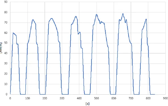
Figure 3 shows the speed profile of route 1 from Table 1. The maximum speed allowed on the track was 80 km/h. However, it was not accelerated to maximum speed between every
station due to the driving style of the driver. Coasting can be seen to be frequently used by the way the curve flattens out on the deceleration part. The acceleration can also be seen to be slowed down before maximum speed was reached between some stations.
Figure 3 Reference case, route one speed profile
Figure 4 shows the speed profile from route two of the reference case. The last stop in Figure 3 is the starting position in Figure 4. They are not exactly mirrored since the track differs a little depending on which direction the train is traveling. The speed profiles in Figure 3 and Figure 4 are the ones emulated in the three cases.
Figure 4 Reference case, route two speed profile
4.3 TEP
To answer the research questions three different variations of simulations will be carried out in TEP. One “all-out” driving, one using the built-in DAS in TEP and one using data from the reference case to create a digital twin in TEP.
This section starts by describing TEP. The train configuration and input data required for simulation can be categorized in eight main sections: train set definition, train unit definition, motor settings, line filter inductor, effort definition, track and environment, schedule and control settings. Then the three cases are explained.
4.3.1 Test conditions
The input data was the same for all three cases.The case conditions were based on the conditions of the reference test to enable a relevant comparison of energy simulation data and actual energy performance data. All input data was provided by Bombardier
Transportation.
4.3.1.1.
Train set definition
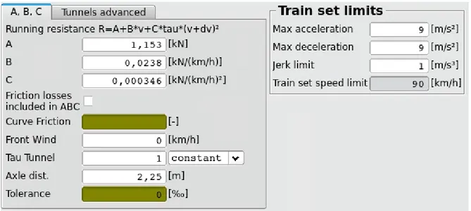
Train set definition includes data on running resistance. The running resistance is calculated in two different ways in TEP. Straight track resistance and curve resistance.
To calculate the straight track running resistance of a train in TEP the Davis formula is used:
Where v is the velocity, A the rolling resistance, B the mechanical resistance, and C the aerodynamic resistance. The coefficients A, B, and C are determined from theoretical
considerations or measurements based on specific conditions and design of train operation. To calculate the curve resistance in TEP the Propapadakis formula is used:
𝐶𝑅(𝑘𝑁) = 𝑔 ∗ 𝑚 ∗𝜇
𝑅∗ (0.72 ∗ 𝑤 + 0.47 ∗ 𝐿) Equation 4
Where μ and w are constants, m the train static weight, L the axle distance, R the curve radius and g the gravitational acceleration. Along with the straight track and curve resistance, the maximum acceleration and minimum deceleration are required to calculate the running resistance. For advanced calculations, specific tunnel data is required since the conditions are very different inside a tunnel than outside.
Figure 5 shows the train set definition of the current study. It is data on the straight track and curve running resistance. The running resistance data was calculated by the vehicle design team at Bombardier Transportation and used in this case. In this degree project, tunnel calculations were excluded from the calculations.
Figure 5 Train set definition
4.3.1.2.
Train unit definition
The train unit definition is data regarding the number of cars, mechanical/electric supply system, train weight, wheel diameter, top speed, passenger load, auxiliary energy supply and more. This data is typically known, and constant for any given train project. If auxiliary energy supply is used, the regenerated energy from braking will first go there before it goes out to the power lines to supply other trains. No auxiliary energy supply was used for this degree project. Also, all braking energy was assumed to be dissipated in brake resistors. Figure 6 shows the train unit definition for the current study. It includes data on the mechanical train unit and the condition of the wheels. The static mass and rotating addon mass were calculated by the vehicle design team at Bombardier Transportation. The rotating addon mass depends on the number of driven axles and the radius of the wheels. The wheels
were half-worn to simulate the average type of wheel condition. No auxiliary power supply was used because the reference case did not use one. Consequently, the train was simulated without the use of climate control. Passenger load was simulated as if 125 people weighing 75 kgs were on board.
Figure 6 Train unit definition
4.3.1.3.
Motor settings
Motor settings in TEP include settings associated with losses in the motor. A harmonic loss profile can be used to include losses associated with the motor but was excluded from this degree project due to a lack of time. The temperatures in the motor are also set here. Figure 7 shows the motor settings for the current study. The temperature in the motor was assumed to be 150 degrees Celsius as commonly used in train performance calculations. The harmonic loss profile can be used to include losses associated with the motor but was
excluded from this degree project due to a lack of time.
Figure 7 Motor settings
4.3.1.4.
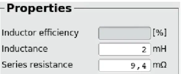
Line filter inductor
Line filter inductor properties include the inductance of the lines used. It is how the currents are filtered from the power supply to the train. Figure 8 shows the line filter inductor
Figure 8 Line filter inductor properties
4.3.1.5.
Effort definition
Effort definition defines the brake and drive power curves. Every train has an individual brake and drives power curve depending on weight, the type of motor used and other train characteristics. Brake and drive power curve are how much power is available for acceleration and braking at different speeds. It also includes how the adhesion of the tracks are, meaning how well the wheels grip the tracks.
The effort definition data was gathered from the reference case data and emulated to fit in the TEP model. Figure 9 shows the total braking, which was constant for all speeds.
Figure 9 Effort definition, total braking
Figure 10 shows the electrical braking curve for the current study. As can be seen in the figure the available power to brake the train decrease at higher speeds due to how the train is
dimensioned. Not enough effort is available at higher speeds, limiting the braking ability of the train.
Figure 11 shows the traction effort definition. The available power to drive the train decrease at higher speeds due to the type of motor used.
Figure 11 Effort definition, traction
4.3.1.6.
Track and environment
Track and environment data are data about the conditions the train is working in. It includes the ambient temperature, line power voltage, and speed limits. The track used a 750 V DC line voltage. There were eight stations, meaning seven stops. The train then switched way and returned on the same track but from the other way. In total there were 14 stops. The cases were simulated one way at a time in order to enable a closer look at the speed profiles and compare them in detail to the reference case. The track used was on an undisclosed urban location. The ambient temperature was set to 10 degrees Celsius. Since the location is hidden more information will not be presented.
4.3.1.7.
Schedule
The schedule includes information of the stations, distances and time limit the train will be active in. The time schedule is important to know when calculating the energy consumption since it creates boundaries the train need to follow. The schedule will not be shown because the location is undisclosed in this degree project.
4.3.1.8.
Control settings
Different control settings can be included for the driving of the train. DAS can be used to minimize energy consumption. A DAS is a system that helps the drivers of the trains to drive the trains in the least energy consuming way possible based on speed profile optimization and scheduling with other trains in service to optimize RB. In TEP it simulates the least energy consuming route on a given time schedule. In real operation, a DAS can give instructions to the drivers who then make proper adjustments. Another tool in TEP is
coasting. Coasting is essentially speeding the train up and then letting it coast when possible, to reduce energy consumption.
4.3.2 Simulations and calculations
To answer the research questions, one track was used to simulate three different driving styles in TEP. In order to calculate the difference in different driving styles, all other parameters must be constant. Data on the train unit, track and environment were constant throughout the three cases.
4.3.2.1.
Case 1: “All-out”
The first case is called “all-out” driving. This simulation calculates how much energy the train uses without any control setting implemented. The train accelerates as much as it can and brakes full when stopping for at a station. This case can be considered the worst-case scenario when the train uses the most energy on a given track set-up.
4.3.2.2.
Case 2: DAS
Case two using the built-in DAS function in TEP required a set time schedule to work in. The DAS constantly makes calculations based on current conditions for the train to calculate the least energy consuming driving style. The exact time scheme including stop times was emulated from the reference case. The driver in the reference case also ignored the 50 km/h speed limit when accelerating from a station, it was therefore removed from the simulations.
4.3.2.3.
Case 3: True operation
To create case three, driving data from the reference case was emulated in TEP. Specifically, the speed profile was analyzed in detail and replicated in TEP. Some top speeds were set lower than the reference case because they were peaks and not easily replicated in TEP. Instead, a lower top speed was considered to better emulate the total speed profile. Coasting settings matched how the train decelerated. To replicate the speed profile of the reference case a trial and error approach was used. Changes were made regarding top speed and
coasting distances and the results were checked towards the reference case speed profile until it was determined to be close enough. However, additional changes should be considered to make the model even better. Since the location is undisclosed, the actual input data will not be presented here.
Figure 12 shows how an example of how a speed profile looks in TEP. The blue curve is the speed limit. It was set to the maximum value the real train achieved between each station to replicate how the real train drives. It decreases to 50 km/h at every station since that is the speed limit around stations. The pink curve shows the speed of the train with respect to the distance.
Figure 12 Typical speed profile in TEP
Table 2 shows how the coasting was emulated in case three. Start position is when the train should start coasting, and the end position is each station stop. Min speed is the minimum speed when coasting should be used, and target speed is the speed the coasting should aim to reach before the station stop. The numbers in Table 2 are only for reference and not the actual numbers used in case three.
Table 2 Coasting set-up
Table 3 shows how the top speed was matched with the real case between every station in TEP. The green column shows the actual speed limits the train can drive according to track limitations. The white columns show how the top speed was matched according to the maximum speeds the real case train had been driving. The numbers in Table 3 are only for reference and not the actual numbers used in case three.
Table 3 Case three top speed set-up
Case three can be considered a replica of the real case when the speed profile, timetable, and train configuration data are the same. Then an accurate comparison of energy data can be performed.
4.4 Maintenance data
To be able to analyze potential benefits of predictive maintenance in urban rail this section covers current maintenance schemes for selected parts from data provided by Bombardier Transportation.
The parameters for maintenance cost are operating time, power-on time and mileage. Operating time refers to the time the component has been in use. Power-on time is the time the part has been powered on, this includes the time when the train is parked but power is still on due to maintenance or cold climate. Mileage is simply the number of kilometers the part has been on the train. There are individual maintenance intervals for each rail project. Table 4 shows one maintenance scheme example for a propulsion system application at Bombardier Transportation. Some of the information has been removed due to privacy reasons. The important information for discussion is the type of part, type, and frequency of maintenance actions. The parts listed in Table 4 are auxiliary power supply, propulsion bearings, internal and external cooling fans of the converter. For this project, they have gotten a set maintenance interval based on an estimated service distance or duration for each component. The interval distances can be seen in the right column in the table. The type of maintenance action is to the left side of the table.
5
RESULTS
This section presents the results of the three case simulations. Then the results are compared. In all speed profile comparisons, the reference case is in blue and the current case is in
orange. The horizontal axis is a time in seconds (s), and the vertical axis is speed in km/h.
5.1
Case 1: “All-out”
Table 5 shows the energy consumption results of case one route one. It includes the total running distance, journey time and total stop time. Net energy use is the energy usage from line minus available regenerated braking energy.
Table 5 Case 1:1 Energy results
Figure 13 shows the speed profile of case one route one in orange and the speed profile of the reference case in blue. Route one is the first eight stations, totaling seven stops. The train accelerated to the max speed of 80 km/h as quickly as possible and then braking as late as possible. This type of driving style can be seen in the figure in the way the curve almost vertically reaches top speed. It then holds that speed until it eventually almost vertically drops before the next stop. It then waits before it starts accelerating again.
Table 6 shows the energy results of case one route two. The distance is a little different in this direction. Some difference is expected due to how the tracks are shaped in each direction.
Table 6 Case 1:2 Energy results
Figure 14 shows the speed profile comparison between case one route two and the reference case. As expected, it is like route one since the only thing different is the direction the train is traveling.
5.2 Case 2: DAS
Table 7 shows the energy results of the first route of the second case when a driver assistance system calculated the most energy efficient driving style in TEP. Case 2:1 means it is route one of case two.
Table 7 Case 2:1 Energy results
Figure 15 shows the speed profile of the first route in this case. As can be seen in the figure the speed varied between each station and on some stations where the distance was too short the max speed of 80 km/h was not achieved. A flatter speed curve also indicates that the train was adjusting the speed and not performing maximum acceleration or braking. Most notably the fourth and fifth orange peak differs from the blue reference case curve. In the fourth peak the simulation is lower than the reference case, resulting in lower energy use. The fifth peak accelerate slower in the simulation, but it also brakes harder with less coasting.
Table 8 shows the energy results of the second route of the second case. This direction is notably less energy intense. It can be because of how the track is shaped with hills and turns.
Table 8 Case 2:2 Energy results
Figure 16 shows the speed profile of the second route in this case. One key difference can be seen in the third peak. In this direction that curve is less vertical, indicating less energy use. Also, the fourth peak is far lower in the simulated orange curve, resulting in lower energy use.
5.3 Case 3: True operation
Table 9 shows the energy results of the third case and first route. This case adapted the maximum speed and coasting between each station to match that of how real trains operate on the track.
Table 9 Case 3:1 Energy results
It also matched the real case speed profile by adapting the coasting settings. The results of the speed profile in the first route in this case in comparison to the reference case can be seen in Figure 17. The speed profile can be seen to follow the reference case very well.
Table 10 shows the energy results for case three route two. As with the third case, the second route in this case used notably less energy than route one.
Table 10 Case 3:2 Energy results
Figure 18 shows the speed profile comparison between case three route two and the reference case. In this direction, the speed profile also followed the reference case very well.
5.4 Energy result comparison
Table 11 shows a comparison of the travel time and energy use between the three simulated cases and the real reference case. Case one was the fastest, but also the most energy
consuming. It was 10 % faster than the reference case and used 31,5 % more energy. Case two used the built-in DAS in TEP and was 23,1 % more energy efficient compared to the reference case on the roundtrip. Both runs in case three matched time compared to the reference case very well. Case three was most like the reference case regarding energy consumption, differing only 0,9 %. Route one was used more energy in both case two and three compared to route two in each respective case. The reference case had the highest average net energy per kilometer and case 2 the lowest.
6
DISCUSSION
This section discusses the three main areas of interest regarding energy efficiency from access to Big data handled in this degree project. First, findings from the literature study are discussed. Then the results from the three cases are examined. Finally, other benefits from access to Big data not related to how the train is driven are reviewed.
6.1 Urban railway energy efficiency and digitalization
Energy-efficient urban railway development is important for big cities as they continue to grow. Because more traffic will result in larger energy consumption and capacity problems for current urban railways. An increasing number of electric buses will compete with urban railways for electricity demand. Developing energy-efficient urban railways require
information on how the trains perform. The information includes temperatures in the cars for better climate control, voltages in the converters to calculate their efficiency and
vibrations in the motor to faster detect wear. It also includes data on train speeds and speed profiles to optimize the driving style of the train. This type of information is not available on a live basis today due to the big data amounts.
New mobile communication technology can handle big data loads while remaining safe from cyber-attacks. There are however several challenges in implementing big data transfer. Big data requires a good data management system. It must be a complex system, able to collect, send and manage Big data loads. The implementations must lead to financial savings or other concrete benefits for companies to perform the necessary investments. Research by Turner et al (2016) shows the most important part of Big data is to interpret the data collected, either by a human or computer. It is first when something useful can be extracted from the bulk of the data that value is created. When implementing such systems there needs to be a high level of adaptability since train projects differ a lot. There are many different types of rail, different passenger loads and climate conditions making it difficult to create one model which suits all projects.
In addition to being able to collect, send and manage big data loads the system must be able to perform calculations faster than current computers can. A research review by
Scheepmaker et al (2017) highlighted the need to simplify the calculations when dealing with Big data loads. Therefore, faster computer technology or making simplifications are required when dealing with Big data loads. If Big data is used to help the driver drive as efficiently as possible with a DAS, another option could be to compute a large set of scenarios offline and then use the solutions in real-time operation. The dilemma is how to create faster
6.2 Better energy and performance simulations
Information on how the train is driven under real conditions is important to make better simulation programs. Improving the simulation programs helps create more realistic
calculations on energy consumption and wear. Therefore, a simulation model was created in TEP based on real driving data. It was then compared to a worst-case driving style and an optimal driving style.
The results indicated that improvements in how the train was driven were possible. Some of the driving characteristics that can be changed can be seen in the speed profile comparison of case two. The speed profiles between said cases are very similar on some distances
confirming the fact that the driver in the real case got help from a DAS system when driving. The DAS generally accelerate much less intensively than the reference case, as can be seen in a steeper curve. A less aggressive acceleration would result in a reduced amount of energy used.
Case three managed to replicate the reference case speed profile and the energy consumption showed to be within 1 % of each other. This indicates that TEP is a reliable tool when
simulating train energy and performance. If Big data was available on for example the speed profile of urban rail operation the performance of the driving style can be analyzed. The DAS simulation in TEP proved to drive more energy-efficiently than the reference case even though they used a simpler form of assisted driving. Therefore, adapting according to coasting and top speeds proved to better predict energy consumption compared to using the DAS in TEP on the same time schedule. Analyzing such data, it might show possible
improvements in implementing a DAS; or it might show no improvement is possible. Either way, it is beneficial for the train operator if some energy saving potential exists, or if they are driving as efficiently as expected.
Case one had almost the same average energy per kilometer as the reference case, due to its low net energy value. Such low net energy presumes that all regenerated braking energy receives by another train or storage station. It also requires the power lines to be able to handle such large power currents. It is therefore unrealistic to assume it to be possible to have such low net energy on case one. Case two had the lowest average energy per kilometer. It is partly due to the DAS taking regenerative braking energy into account when calculating the most energy efficient driving style. Regenerative braking has been studied by Kılıçkıran, et al (2017) and found to be able to drastically reduce the net energy used by a train. A DAS tries to maximize the amount of regenerative braking possible and is therefore important to use when driving a train. Case three was in between the other two simulated cases. It still had a lower net energy consumption than the reference case. This could be because the losses measured in the reference case are higher than the ones simulated in TEP.
Some sources of error include tunnel data simulation. In the simulations the tracks were excepted from tunnel data information, meaning they were simulated as if there existed no tunnels on the tracks. The conditions inside a tunnel are very different from outside, a train traveling through a tunnel will for example experience much more motion resistance
compared to outside a tunnel. If accurate tunnel data information had been implemented the results would have been considered more accurate due to the simulated losses would have
been closer to the reference case. No harmonic loss profile was included in the motor
settings. Although not as important as tunnel data, the inclusion of the harmonic loss profile would have resulted in more realistic simulations since the real motor performance would have been better matched to the one from the reference case. The motor temperature is almost always set to 150 degrees Celsius in train energy and performance calculations. However, the actual motor temperature varies throughout the driving cycle. Even though the average motor temperature might be close to 150 degrees Celsius, the actual temperature might be lower at the start of a cycle. The motor temperature will also vary depending on the time of day the train is active since the outside temperature will vary during every day. Motor temperature data was not available for this degree project, but if it had been the simulations would be considered more accurate. Because the reference case motor temperature varied and therefore losses are different from a constant temperature calculation.
TEP uses simplified models of the motor and converter. More accurate models exist in other tools at Bombardier Transportation for more detailed design and analysis of converters and motors. Therefore, more complete and detailed loss analysis is possible but would require more extensive iterations. It might be worthwhile considering a simplified and automated means for data exchange between TEP and the other tools to speed up the optimization process.
6.3 Other energy optimization implementations
There are several other parts of urban railway operation which could benefit from access to true operation data. The implementation of preventive maintenance actions is one of the most interesting cases of true operation data since it can be implemented on the current rolling stock without major investments by using existing sensors. The sensors were found to accurately measure energy performance. Predictive maintenance can minimize unplanned downtime by detecting faulty parts before they break. Since corrective maintenance is the most expensive kind of maintenance minimizing it would lead to lower maintenance costs. On the other side fully, functional parts are unnecessarily being replaced due to a planned or condition-based maintenance strategy.
One example of a maintenance scheme is the internal and external cooling fans of the converter, which are replaced based on how many kilometers the train has rolled instead of their actual level of wear. Today they are changed based on an estimated service distance or duration. Since every rail project is different, and the working conditions for each train may vary from the theoretically considered conditions, the intervals will be hard to get right. Ideally, each part should be replaced just before failure, to maximize lifetime and minimize failure. Using parts to their true, full life length will lead to both energy and economic savings by minimizing the number of maintenances stops and new part purchases. Implementation of such maintenance schemes will have investment costs which need to be motivated by the potential benefits of preventive maintenance.
Better access to operational data for different components and subsystems would also benefit root cause analysis of common problems enabling corrective measures to be implemented in