Particles in road and railroad tunnel air : sources, properties and abatement measures

Mats Gustafsson

Saeed Abbasi

Göran Blomqvist

Yingying Cha

Anders Gudmundsson

Sara Janhäll

Christer Johansson

Michael Norman

Ulf Olofsson

Particles in road and railroad tunnel air

Sources, properties and abatement measures

VTI r apport 917A | P articles in r oad and r ailr

oad tunnel air

. Sour

ces, pr

operties and abatement measur

www.vti.se/en/publications

VTI rapport 917A

Published 2016

VTI rapport 917A

Particles in road and railroad tunnel air

Sources, properties and abatement measures

Mats Gustafsson

Saeed Abbasi

Göran Blomqvist

Yingying Cha

Anders Gudmundsson

Sara Janhäll

Christer Johansson

Michael Norman

Ulf Olofsson

Diarienummer: 2012/0663-242

Omslagsbilder: Thinkstock, Mats Gustafsson Tryck: VTI, Linköping 2016

Abstract

High levels of air pollution are a common problem in both road and railroad tunnels. Sources and emission processes however differ significantly, as reflected by aerosols physical and chemical

properties. As particle concentrations and properties affect exposure of and health effects for people on platforms and in vehicles, effective ways to reduce emissions and exposure are important. This study aims to improve the knowledge of the differences between PM10 in the rail and road tunnel

environments, their sources and the possibilities to address problems with high particulate levels. Measurement campaigns were carried out at Arlanda Central, a railroad tunnel station below Arlanda airport and in Söderleden road tunnel, a road tunnel in central Stockholm.

The results show large differences in concentration levels, size distributions and in composition of the particles. The railroad tunnel aerosol consisted of coarse particles with high iron content, while the properties of the coarse particles in the road tunnel were strongly influenced by whether the road surface was wet or dry. In wet conditions, concentrations were relatively low and iron and sulfur dominating elements, while silicon, potassium, calcium and iron from suspension and road wear dominated during dry conditions. The content of elemental carbon, most likely from the pantograph, were unexpectedly high in the railroad tunnel. An older type of train with a large proportion of mechanical brakes were suggested to be responsible to the main particle emissions in the railway tunnel. The report concludes with a discussion and proposals for action against particle sources in the various underground environments.

Title: Particles in road and railroad tunnel air. Sources, properties and

abatement measures

Author: Mats Gustafsson (VTI)

Saeed Abbasi (KTH) Göran Blomqvist (VTI) Yingying Cha (KTH)

Anders Gudmundsson (Lund University) Sara Janhäll (VTI)

Christer Johansson (SLB-analys and Stockholm University) Michael Norman (SLB-analys) and Ulf Olofsson (KTH)

Publisher: Swedish National Road and Transport Research Institute (VTI).

www.vti.se

Publication No.: VTI rapport 917

Published: 2016

Reg. No., VTI: 2012/0663-242

ISSN: 0347-6030

Project: Particle emissions in road and railroad tunnels

Commissioned by: BVFF

Keywords: Tunnel, PM10, PM2.5, ultrafines, size distribution, NOx, train, car, road,

railroad, abatement

Referat

Höga halter av luftföroreningar är ett vanligt förekommande problem i tunnlar för såväl väg som järnväg. Källor och emissionsprocesser skiljer sig dock åt väsentligt, vilket avspeglas i aerosolernas fysikaliska och kemiska egenskaper. Då partiklarnas halter och egenskaper är viktiga för exponering och hälsoeffekter för människor på perronger och i fordon, är effektiva sätt att minska emissionerna och exponeringen av vikt. Föreliggande studie syftar till att förbättra kunskapen om skillnaderna mellan inandningsbara partiklar (PM10) i väg och järnvägsmiljö, partiklarnas källor och möjligheterna att åtgärda problem med höga partikelhalter. Mätkampanjer genomfördes på Arlanda Central, en järnvägsstation under Arlanda flygplats och i Söderledstunneln, en vägtunnel i centrala Stockholm. Resultaten visar på stora skillnader i såväl halter och storleksfördelningar som i partiklarnas samman-sättning. I järnvägstunneln utgjordes aerosolen av grova partiklar med högt järninnehåll, medan egen-skaperna hos de grova partiklarna i vägtunneln påverkades starkt av om vägbanan var våt eller torr. Vid våt vägbana var halterna förhållandevis låga och järn och svavel viktiga element, medan kisel, kalium, kalcium och järn från suspension och vägslitage dominerade vid torr vägbana. Halten av elementärt kol, sannolikt från strömavtagare, var oväntat hög i järnvägstunneln. En äldre tågtyp med stor andel mekaniska bromsar bedömdes orsaka huvuddelen av partikelemissionerna i järnvägs-tunneln. Rapporten avslutas med en diskussion om och förslag till åtgärder mot partikelkällor i de olika tunnelmiljöerna.

Titel: Partiklar i väg- och tågtunnelluft. Källor egenskaper och

åtgärdsmöjligheter.

Författare: Mats Gustafsson (VTI)

Saeed Abbasi (KTH) Göran Blomqvist (VTI) Yingying Cha (KTH)

Anders Gudmundsson (Lunds universitet) Sara Janhäll (VTI)

Christer Johansson (SLB-analys och Stockholms universitet) Michael Norman (SLB-analys)

Ulf Olofsson (KTH)

Utgivare: VTI, Statens väg och transportforskningsinstitut

www.vti.se

Serie och nr: VTI rapport 917

Utgivningsår: 2016

VTI:s diarienr: 2012/0663-242

ISSN: 0347-6030

Projektnamn: Partikelemissioner i väg- och järnvägstunnlar

Uppdragsgivare: BVFF

Nyckelord: Tunnel, PM10, PM2.5, ultrafina partiklar, storleksfördelningar, NOx,

tåg, bilar, väg, järnväg, åtgärder

Språk: Engelska

Preface

This project was initiated as an application to BVFF, an industry programme for research, development and innovations in road and railway construction and maintenance, in 2012. Field campaigns were conducted in first half of 2013. Part of the work was conducted as part of Saeed Abbasi’s Ph.D. studies. The authors would like to thank Håkan Wilhelmsson and Stig Englund for managing the traffic measurement system at Arlanda, Anna Kryhl at the Swedish Transport Authority for supplying railroad traffic data and finally Göran Lidén at ACES, Stockholm University, for valuable comments on the manuscript.

Linköping, in November, 2016

Mats Gustafsson Project leader

Quality review

External peer review was performed on 30 July 2016 by Göran Lidén, Department of Environmental Science and Analytical Chemistry (ACES), Stockholm University. Mats Gustafsson has made alterations to the final manuscript of the report. The research director Mikael Johannesson examined and approved the report for publication on 21 November 2016. The conclusions and recommendations expressed are the authors’ and do not necessarily reflect VTI’s opinion as an authority.

Kvalitetsgranskning

Extern peer review har genomförts 30 juli 2016 av Göran Lidén, Institutionen för miljövetenskap och analytisk kemi (ACES), Stockholms universitet. Mats Gustafsson har genomfört justeringar av slutligt rapportmanus. Forskningschef Mikael Johannesson har därefter granskat och godkänt publikationen för publicering 21 november 2016. De slutsatser och rekommendationer som uttrycks är författarnas egna och speglar inte nödvändigtvis myndigheten VTI:s uppfattning.

Content

2.1.1. Arlanda C – railroad tunnel ...15

2.1.2. Söderleden road tunnel ...18

2.2. Measurements ...19

2.2.1. PM10 ...20

2.2.2. Size distribution measurements and particle sampling ...20

2.2.3. NOx ...21

2.2.4. EC/OC ...21

2.2.5. Element analysis ...22

2.2.6. Data from and measurements made on X60 commuter train ...22

3. Results ...24

3.1. Traffic characteristics ...24

3.1.1. Arlanda C ...24

3.1.2. Söderleden road tunnel ...26

3.2. Particle and NOx concentrations (TEOM, NOx, CPC) ...28

3.2.1. Temporal patterns in the Arlanda C railroad tunnel and relation to traffic and meteorology ...28

3.2.2. Temporal patterns in the Söderleden road tunnel and relation to traffic and meteorology ...33

3.3. Particle size distributions (APS, SMPS, ELPI) ...39

3.3.1. Detailed studies of train type (individual) effects at Arlanda ...43

3.4. EC/OC ...52

3.5. Size segregated element composition ...54

3.6. Results from on-board measurements from a X60 train ...62

4. Synthesis and discussion ...66

4.1. Identification of the main PM sources ...66

4.1.1. Railroad tunnel ...66

4.1.2. Road tunnel ...69

4.2. Abatement of identified sources ...70

4.2.1. Railroad tunnel ...70

4.2.2. Road tunnel ...71

4.3. Future work ...73

Summary

Particles in road and railroad tunnel air. Sources, properties and abatement measures

by Mats Gustafsson (VTI), Saeed Abbasi (KTH), Göran Blomqvist (VTI), Yingying Cha (KTH) Anders Gudmundsson (Lund University), Sara Janhäll (VTI), Christer Johansson (SLB-analys and Stockholm University), Michael Norman (SLB-analys) and Ulf Olofsson (KTH)

High levels of air pollution are a common problem in both road and railroad tunnels. However, sources and emission processes differ significantly, as reflected by the physical and chemical

properties of the two aerosols. As particle concentrations and properties affect exposure of and health effects for people on platforms and in vehicles, effective ways to reduce emissions and exposure are important. This study aims to improve the knowledge of the differences between PM10 in the rail and road tunnel environments, their sources and the possibilities to address problems with high particulate levels.

Measurement campaigns were carried out at Arlanda Central, a railroad tunnel station below Arlanda airport and in Söderleden road tunnel, a road tunnel in central Stockholm. Measurements included particle concentrations, size distributions, size resolved element content, NOx, and organic and

elemental carbon. Traffic and meteorology were measured and/or collected from existing databases. In Söderleden road tunnel, the campaign (non-intentionally) included both a period that was mainly wet and one that was dry. This gave the opportunity to study the differences in the importance of

suspension to the contribution to particle levels.

The results show that the rail tunnel environment was characterized by relatively high concentration peaks of coarse particles and low levels of NOx and NO2. Some trains were linked to emissions of ultrafine particles. The composition of the airborne particles is dominated by iron, with smaller contributions from copper, zinc and other metals. The road tunnel is characterized by high levels of ultra-fine particles, NOx and NO2 and, in dry condition, also high levels of coarse particles. As the traffic is more intense than in the rail tunnel, particle levels are more constantly high during busy traffic. In humid conditions the coarse particles were dominated by iron whereas particles below about 1 micron were dominated by sulfur. In dry conditions, increases in the typical mineral elements silicon, potassium, calcium and iron were substantial. Chlorine represents a significant percentage in both wet and dry conditions, which suggests a contribution from road salt. The iron is suggested to originate from brake were in wet conditions, and from both brake wear and road wear in dry

conditions. By comparing the data with train passages and information on train types, it was found that most of the high particulate levels recorded at Arlanda C are correlated to older trains with

locomotives of type Rc with their wagons. These mainly have mechanical brakes and are also braked during longer time and distance before stopping at the station. The content of elemental carbon in the air of the railroad environment was unexpectedly high, about half of the content of the road tunnel, despite lack of combustion sources. This is considered to be due to wear of graphite from the train pantograph. The main focus of action against high particle levels in railroad tunnels has been on ways to prevent exposure by separating trains from the platform or to vent contaminated air, while studies on the opportunities to prevent emissions are fewer. This study demonstrates the potential to reduce particulate emissions by identifying the types of trains and train individuals and their characteristics, technical systems that causes particle emissions, maintenance status and also how they are driven. In road tunnels abatement measures against coarse particles are linked to measures that reduce studded tire wear of road surface or reduce the suspension of deposited dust. This can be done by reducing the use of studded tires, improved pavements, effective dust control and cleaning, in addition to reducing traffic and speed. The ultrafine particles present in high concentrations originate from vehicle exhaust

Sammanfattning

Partiklar i väg- och järnvägstunnlar. Källor, egenskaper och åtgärder.

av Mats Gustafsson (VTI), Saeed Abbasi (KTH), Göran Blomqvist (VTI), Yingying Cha (KTH), Anders Gudmundsson (Lunds universitet), Sara Janhäll (VTI), Christer Johansson (SLB-analys och Stockholms universitet), Michael Norman (SLB-analys) och Ulf Olofsson (KTH)

Höga halter av luftföroreningar är ett vanligt förekommande problem i tunnlar för såväl väg som järnväg. Källor och emissionsprocesser skiljer sig dock åt väsentligt, vilket avspeglas i aerosolernas fysikaliska och kemiska egenskaper. Då partiklarnas halter och egenskaper är viktiga för exponering och hälsoeffekter för människor på perronger och i fordon, är effektiva sätt att minska emissionerna och exponeringen av vikt. Föreliggande studie syftar till att förbättra kunskapen om skillnaderna mellan inandningsbara partiklar i väg- och järnvägsmiljö, partiklarnas källor och möjligheterna att åtgärda problem med höga partikelhalter.

Mätningar genomfördes på Arlanda Central, en järnvägsstation under Arlanda flygplats och i Söderledstunneln, en vägtunnel i centrala Stockholm. Mätningar gjordes av partikelhalter, storleks-fördelningar, storleksuppdelat elementinnehåll, NOx och organiskt och elementärt kol. Trafik och meteorologi mättes och/eller inhämtades från befintliga databaser. I Söderledstunneln inföll mätningarna under en period som var i huvudsak fuktig och en som var i huvudsak torr, vilket gav möjlighet att studera betydelsen av bidraget från suspension till partikelhalterna.

Resultaten visar att järnvägstunnelmiljön präglas av relativt höga koncentrationstoppar av grova partiklar och låga halter NOx och NO2. Vissa tåg kan kopplas till emissioner av ultrafina partiklar. Partiklarna domineras innehållsmässigt av järn, med mindre bidrag av koppar, zink och andra metaller. Vägtunneln präglas av höga halter ultrafina partiklar, NOx och NO2 och, under torra förhållanden, även höga halter grova partiklar. Då trafiken är mer intensiv än i järnvägstunneln är halterna mer konstant höga under trafikerad tid. Under fuktiga förhållanden domineras de grova partiklarna (PM2.5– 10) av järn medan partiklar under cirka 1 µm domineras av svavel. Under torra förhållanden ökar de mineraltypiska elementen kisel, kalium, kalcium och järn kraftigt. Klor utgör en betydande andel under både fuktiga och torra förhållanden vilken tyder på ett bidrag från vägsalt. Järnet bedöms härröra från bromsar under fuktiga förhållanden och från både bromsar och vägslitage under torra förhållanden.

Genom att jämföra data med tågpassager och tågtyper, konstaterades att huvuddelen av de höga partikelhalter som registreras på Arlanda C kan kopplas till äldre tåg av typen RC. Dessa är främst mekaniskt bromsade och bromsas även under längre tid och sträcka innan de stannar vid stationen. Halten elementärt kol i luften i järnvägsmiljön var oväntad hög, ungefär hälften av halten i vägtunneln, trots avsaknad av förbränningskällor. Detta bedöms bero på slitage av grafit från tågens strömavtagare. Huvudsakligt fokus på åtgärder mot höga partikelhalterna i järnvägstunnlar har legat på sätt att

förhindra exponering genom att skilja av tågen från perrongen eller att ventilera ut förorenad luft, medan studier kring möjligheter att förhindra själva emissionen är få. Föreliggande studie visar på potential att reducera partikelemissioner genom att identifiera tågtyper och enskilda tåg och deras egenskaper, tekniska system som medför partikelemissioner, underhållsstatus och även hur de framförs. I vägtunnlar är åtgärdsmöjligheterna mot grova partiklar kopplade till åtgärder som minskar dubbdäcksslitaget av vägytan eller minskar suspensionen av bildat damm. Detta kan ske genom minskad dubbdäcksanvändning, förbättrade beläggningar, effektiv dammbindning och städning, förutom genom trafikåtgärder som minskad trafik och hastighet. De ultrafina partiklar (<100 nm) som förekommer i höga koncentrationer härrör från fordonsavgaser och kan (förutom genom fortsatta regleringar av utsläpp från fordon) endast åtgärdas genom trafikåtgärder som minskad trafikmängd

1.

Background

Air pollution in road tunnels is a well-known problem. Exhaust gases and combustion related particles reach far higher concentrations than in street or road environments. A very large number of studies have analysed the air quality in road traffic tunnels, e g in Stockholm (Kristensson et al., 1999), Gothenburg (Sternbeck et al., 2002), Switzerland (Weingartner et al., 1997), California (Kirschstetter et al., 1999), Austria and the UK (Imhof et al., 2006). Typically, both the morphological, chemical and physical properties of the aerosol differ substantially between rail and traffic road tunnels. Incomplete combustion of vehicle fuels lead to high concentrations of ultrafine particles in road tunnels, which is normally not present in rail tunnels. Super-micron particles generated during mechanical wear processes are present in both environments, but with very different chemical composition due to the different processes and materials involved in the generation of these particles. Also, the gaseous air pollutant mix differ substantially. While NO and NO2 are normally high in road tunnels during traffic hours, these gases are at background level in railroad tunnels, except when trafficked by maintenance diesel powered vehicles (Han et al., 2015).

Even though not trafficked by combustion vehicles, high levels of particulate air pollution have been recognized in several subway stations, e g Stockholm, London, New York city, Tokyo, Helsinki, Mexico City, Taipei, Prag, Budapest, Seoul and Rome (Aarnio et al., 2005; Birenzvige et al., 2003; Johansson and Johansson, 2003; Ripanucci et al., 2006; Seaton et al., 2005, Nieuwenhuijsen et al 2007, Kim et al, 2008, Raut et al.,2009; more references are given in Abbasi et al. (2013) and

Järvholm et al., 2013). The particle mass concentrations (PM10 and PM2.5) are generally several times higher than in the most polluted street environments and range from tens to several hundreds of micrograms per cubic meter, depending on traffic amounts and ventilation situation.

Norman and Johansson (2005) and later Midander et al. (2012) established that the number

concentration of particles was about five to ten times lower in the subway than in a densely-trafficked street environment (Hornsgatan, Stockholm). Tokarek et al. (2002) concluded that 99 % of the number of particles were smaller than 2.5 µm and that 50–60 % were smaller than 0.35 µm. This is not

contradicting the fact that the mass concentration, as mentioned above, is higher in railroad tunnel than street environments due to the mass’ cubical dependency of particle radius. The influence of vehicle exhaust emissions on air quality in the subway will of course vary depending on the ventilation etc. Most of the PM10 from emissions in railroad environments consist of different oxidized forms of iron. In a Stockholm subway station, around 60 % of the PM10 was found to be iron or iron oxides, both magnetite (Fe3O4) and hematite (Fe2O3) (Johansson, 2005). Many other trace metals and metalloids have been found in elevated concentrations in subway environments, e g chromium, nickel, arsenic, calcium, barium, copper, antimony and aluminium (e g Querol et al., 2012). Also, organic material has been identified.

Based on a source receptor analysis of chemically speciated filter samples from Stockholm subway and measured composition of rails, brakes etc., Johansson (2005) found that the largest contribution (70 %) to PM10 was due to wear of wheels and/or rail. The rest was mainly brake wear material. Due to the high concentrations of PM10 in subway environments, there is a concern that high

concentrations might be found also in regular railroad environments, where many travellers and train and rail personnel are exposed.

There are much fewer particle measurements in ground level railroad environments compared to subways (Järvholm et al., 2013). Gehrig et al. (2007) measured the PM10 concentration close to the tracks of the railroad station in Zurich, Switzerland. They found a small but significant contribution to long-term average PM10 concentrations (about 1 µg m-3) mainly consisting of iron, but also with contributions from copper, manganese and chromium from the railroad. Bukowiecki et al. (2007)

PM10 concentrations on platforms of 4 ground level stations in Sweden and concluded that none of the environments risked to exceed the EU limit values.

Concentrations and characteristics of inhalable particles from different sources are of great interest since these particles have been shown to cause health effects in the population. The health effects of particles generated in railroad environments are not well known, but some studies have been performed. A comprehensive review has recently been made by Järvholm et al. (2013).

Järvholm et al. (2013) compared the health risks of exposures in subway and railroad tunnels with risks due to exposures in road traffic tunnels and discussed possible metrics to be used to regulate air quality in railroad tunnels. Based on the different air pollution mixtures in the different tunnel environments as well as health studies (including toxicological studies, experimental studies on humans and animal studies), they conclude that health risks are likely larger for exposures in road traffic compared to railroad tunnels, but also that rather few health studies are available.

Some results concerning railroad particles reviewed by Järvholm et al. (2013) and by Gustafsson (2009) are referred in the following. Chillrud et al. (2005) have compiled the health effects of iron, manganese and chrome, which are among the most enriched metals in subway environments. Iron is suspected to have negative health effects because of its capacity to form free radicals, which has been connected to diseases such as Parkinsonism, Alzheimer’s and multiple sclerosis. Manganese poisoning is known to cause Parkinsonism, while chromium is a well-known carcinogen. There is no

epidemiological evidence, however, that relatively low exposure to these metals in subway air is related to these diseases.

A cell study using PM10 particles from a Stockholm subway station showed that the iron rich particles were 8 times more genotoxic and 4 times more likely to cause oxidative stress in lung cells than PM10 from an urban street environment (Karlsson et al., 2006; Karlsson et al., 2005). The higher

genotoxicity is most likely caused by highly reactive surfaces giving rise to oxidative stress (Karlsson et al., 2008). On the other hand, a simultaneous cell study focusing on inflammation potential

concluded that PM10 particles from the subway were less inflammatory for human macrophages than city street PM10 (Lindbom et al., 2006, Gustafsson et al., 2008).

In 2008 an epidemiological study concluded that lung cancer incidence was not increased among subway drivers in Stockholm, Sweden, claiming this result gives some evidence against the hypothesis that subway particles would be more potent in inducing cancer than other particles in ambient air (Gustavsson et al., 2008).

Klepczynska Nyström et al. (2010) exposed healthy volunteers to a subway environment and a control environment (office) and found no significant differences in lung function or in inflammatory

response. Significant effects were however found in blood where fibrogene and regulatory T-cells increased. This is the very first published controlled human exposure study of subway particles. For road tunnel environments, there are some human experimental studies made in Stockholm, but otherwise it seems that there are not as many studies as for subway tunnels (see Järvholm et al., 2013). Svartengren et al (2000) showed that exposure to air pollution in road tunnels may significantly enhance asthmatic reactions to subsequently inhaled allergens. Larsson et al. (2007) showed that a 2-hour exposure of healthy subjects to traffic pollution in the same road tunnel resulted in increased inflammatory response in lower airways, but no increase in blood coagulation factors, cellular infiltration or effects on lung function were seen.

The aim of this study was to measure, characterize and investigate the differences in particle properties in a road and a railroad tunnel and to identify their main sources to be able to suggest relevant and effective measures to reduce high particle concentrations.

2.

Methodology

2.1.

Tunnel sites

2.1.1. Arlanda C – railroad tunnel

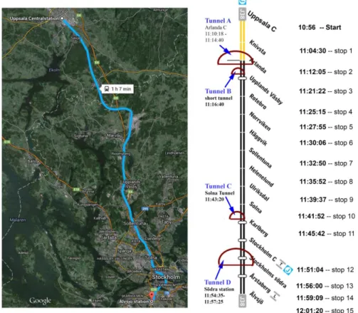
The subterrainean station Arlanda Central (C) is situated north of Stockholm below Arlanda airport. The platform is 400 m long with one track on either side with traffic in opposite directions. The tunnel is approximately 5 km long and the station is trafficked by mixed long distance, regional and

commuter trains passing the airport. The tunnels are self-ventilated. The only active ventilation is smoke evacuation fans only activated if fire occurs.

Figure 1. Arlanda tunnel and its entrances (upper) and Arlanda C platform with placement of the measurements.

The traffic in the tunnel is a mix of electrical trains, from long distance to commuter trains of different age and construction (Figure 2).

Figure 2. Train types trafficking Arlanda C. All photos from järnväg.net.

Apart from these electric trains, different types of maintenance vehicles traffic the tunnel, mainly in night time, when there is no regular train operations ongoing. These vehicles can be either electrically or diesel driven.

The train traffic at Arlanda C was measured by a photocell equipment designed at VTI registering each train arrival approximately 10 meters from the Arlanda C train station platform at each track (track 1= northbound, track 2 = southbound). The two rays were placed perpendicular to the rail, hence the speed could be calculated using equation 1 and 2:

𝐹𝑟𝑜𝑛𝑡 𝑆𝑝𝑒𝑒𝑑 = 2

𝑇𝑟𝑎𝑦2𝑑𝑖𝑠−𝑇𝑟𝑎𝑦1𝑑𝑖𝑠 (equation 1)

𝐴𝑓𝑡 𝑆𝑝𝑒𝑒𝑑 = 2

𝑇𝑟𝑎𝑦2𝑟𝑒𝑠−𝑇𝑟𝑎𝑦1𝑟𝑒𝑠 (equation 2)

where Tray1dis is the timing at when the first ray is disrupted, Tray2dis is the timing at when the second ray is disrupted, Tray1res is the timing at when the first ray is resumed and Tray2res is the timing at when the second ray is resumed.

Since both the train front speed (by disrupting the rays) and train aft speed (by resuming the rays) could be calculated, the train length (equation 3) and speed retardation (equation 6) could be

calculated using equation 4 and 5 for calculating the mean timing of the front and aft speed, i.e. when the train front and aft are exactly in the mid-point between ray 1 and ray 2.

Photo: Fredrik Tellerup Photo: Markus Tellerup

Photo: Katarina Sandberg

Photo: Fredrik Tellerup Photo: Fredrik Tellerup

X2

X40

X50-55

𝑇𝑟𝑎𝑖𝑛 𝑙𝑒𝑛𝑔𝑡ℎ = 𝐹𝑟𝑜𝑛𝑡 𝑠𝑝𝑒𝑒𝑑+𝐴𝑓𝑡 𝑠𝑝𝑒𝑒𝑑 2 × (𝑇𝑎𝑓𝑡 𝑠𝑝𝑒𝑒𝑑− 𝑇𝑓𝑟𝑜𝑛𝑡 𝑠𝑝𝑒𝑒𝑑) (equation 3) 𝑇𝑓𝑟𝑜𝑛𝑡 𝑠𝑝𝑒𝑒𝑑 = (𝑇𝑟𝑎𝑦1𝑑𝑖𝑠+ (𝑇𝑟𝑎𝑦2𝑑𝑖𝑠−𝑇𝑟𝑎𝑦1𝑑𝑖𝑠) 2 ) (equation 4) 𝑇𝑎𝑓𝑡 𝑠𝑝𝑒𝑒𝑑 = (𝑇𝑟𝑎𝑦1𝑟𝑒𝑠+ (𝑇𝑟𝑎𝑦2𝑟𝑒𝑠−𝑇𝑟𝑎𝑦1𝑟𝑒𝑠) 2 ) (equation 5) 𝑅𝑒𝑡𝑎𝑟𝑑𝑎𝑡𝑖𝑜𝑛 =𝐴𝑓𝑡 𝑠𝑝𝑒𝑒𝑑−𝐹𝑟𝑜𝑛𝑡 𝑠𝑝𝑒𝑒𝑑_𝑇 𝑎𝑓𝑡 𝑠𝑝𝑒𝑒𝑑−𝑇𝑓𝑟𝑜𝑛𝑡 𝑠𝑝𝑒𝑒𝑑 (equation 6)

The photocells (brand: IR transmitter IFM Efector 200 OA5101, IR receiver IFM Efector 200

OA5102) were fixed two meter apart on aluminium rods held by two tripods at approximately 130 cm above the rails (Figure 3). The timing of ray disruption and resuming was logged by a TA89-logging equipment (VTI notat T147).

During the measurement period 2013-01-28–2013-02-11, a total of 885 northbound and 959 southbound train arrivals were registered.

Train definitions used in the data analyses are: Length 20–400 m, acceleration/retardation between 2 and -2 m s–2, front speed above 2 m-s_.

Figure 3. Train traffic counting equipment in the tunnel. Measurement rays across the rail is indicated by red lines in the photo.

2.1.2. Söderleden road tunnel

Söderleden road tunnel in central Stockholm is 1.5 km long and is unidirectional in two separated bores, each bore with traffic distributed over two lanes. In this study measurements were made in the southbound tunnel bore, ca 1060 meters from the north entrance. The tunnel bore has a slight

downward slope from the entrance to the sampling point. The tunnel is ventilated through two ventilation towers (see Figure 5).

Figure 4. Söderleden road tunnel. Arrows indicate main tunnel entrances.

Figure 5. Ventilation situation in Söderleden road tunnel. The idea with the ventilation slot is that northbound air should return in the southbound tunnel tube and be ventilated in the tower at Skansbrogatan. This is to avoid polluted air from exiting through the northern tunnel opening.

Unfortunately, there are no traffic counting inside the tunnel, but traffic is recorded by the congestion charge portal on a bridge (Johanneshovsbron), which is directly connected to the tunnel.

Northbound traffic Southbound traffic Ventilation slot Ventilation tower Ventilation tower AQ measurements Traffic measurements

2.2.

Measurements

Measurements were performed between 2013-02-12 and 2013-03-06. An overview of instruments used and parameters measured is given in Table 1, followed by more detailed descriptions in sub-chapters.

Table 1. Instruments used during the campaign.

Instrument Parameter Arlanda C railroad tunnel Söderleden road tunnel Mobile measurements on X60 Commuter train R&P TEOM PM10 X X AC31M Thermo Electronics

NO, NO2, NOx

X X

TSI APS 3321 Particle size distribution (aerodynamic) 0,523 - 14,6 µm

X X

TSI OPS 3330 Particle size distribution(optical) 0,3 - 10 µm

X

TSI SMPS 3080 Particle size distribution (mobility) 14,6 - 661,2 nm X X TSI SMPS Nanoparticle Sizer 3910 Particle size distribution 10 - 420 nm X

TSI FMPS 3091 Particle size distribution (mobility) 5,6 - 560 nm

X

TSI CPC 3022 Particle number concentration (mobility) 7 nm - ~1 µm

X X

ELPI+ Particle size distribution (aerodynamic) 6 nm - 10 µm 14-stage particle sampler X X Leckel SEQ 47/50 Sampling on filters for analyses of EC/OC X X

2.2.1. PM10

Monitoring of PM10 was performed using tapered element oscillating microbalance (TEOM) instruments (Thermo Fischer Inc., USA, model 1400a). The inlet at Arlanda were placed 2 m above the platform. Due to installation difficulties, a vertical inlet could not be used in the road tunnel. There were probably some losses in the inlet tubing to the TEOM, but these were not estimated further. The PM10 levels in the road tunnel are therefore most likely underestimated. The inlet in Söderleden road tunnel was placed 2.5 m above the road. The TEOM was logged with one minute time resolution.

2.2.2. Size distribution measurements and particle sampling

Particle size distributions were measured using TSI Aerodynamic Particle Sizer (TSI APS 3321) and Scanning Mobility Particle Sizer (TSI SMPS 3080). These instruments measure, in tandem, the particle number distribution in the size range 7 nm – 18 m. SMPS measures over the range 14,6-661,2 nm, and the measurement results are presented as particle number distribution, while the coarser particles are measured with APS over the range 0.523-14,6 m and are presented as mass distribution. The reason for this is that submicron particles are best represented by number since they have very low mass in relation to the coarse particle fraction. The time resolution for APS was 20 s, while the SMPS was set to 90 s. In the conversion from number to mass, a particle density of 5,000 kg m-3 _{is used for} particles > 0.5 m in the railroad tunnel (density of iron oxide) and for smaller particles a particle density of 1,000 kg m-3_{. In the road tunnel the APS used a density for 2,800 kg/m}3_{, which is a} representative density for rock. For APS the Stokes correction was used which corrects for APS's overestimate of the particle size when the particle density is much higher than 1,000 kg m-3_{. Total} particle number were measured using a TSI CPC 3022. It covers the size range from 7 nm and upwards. It was measured with 1-minutes time resolution.

Complementing, shorter measurements of size distributions and size fractionated sampling of particles were made using Dekati ELPI+ and TSI fast mobility particle sizer spectrometer (FMPS 3091. The ELPI+ is an electrical low pressure impactor Dekati model ELPI+ referred to hereinafter as ELPI. This device composed to 15 stages and measured real time PM10, PM2.5 and particle size distribution (PSD) of airborne particles in 14 channels from 6 nm to 10 µm in aerodynamic diameter. The data acquisition can be set to either 1 or 10 Hz according to the operator’s desire. Also, it enables collection of samples on 25-mm-diameter polycarbonate filters in 14 size fractions to do further chemical investigation. The instrument was set to a sampling frequency of 10 Hz and a particle density of 1000 kg m-3, _{based on} resultsfrom laboratory studies on airborne brake wear particles (Ulf Olofsson, oral communication, 2016). In order to eliminate any bouncing effects, all filters were coated by DS-515 grease spray before mounting in ELPI stages. During each coating process, we kept one coated filter as laboratory blank filter to compare the blank filter with the field filters. The sampling airflow was 10 lpm in ELPI. The (FMPS), TSI model 3091 is referred to hereinafter as FMPS. The FMPS measured PSD of submicron particles from 5.6 nm to 560 nm in diameter in 32 channels every second. Its sampling flow rate was 10 lpm and the particle density was set to 1000 kg m-3_.

Figure 6. Some of the instrumentation used in the Söderleden road tunnel.

2.2.3. NOx

NOx including both NO and NO2, were measured using the chemiluminescence analyzer AC31M from Thermo Electronics. The instrument measures NO and NOx while the NO2 concentrations are

calculated automatically from the measured values. The inlet was placed 2 m above the platform at Arlanda and 2.5 m above the road in Söderleden road tunnel. The NOx values were logged with a 1-minute time resolution.

2.2.4. EC/OC

Aerosol samples are collected on quartz-fibre filters (Munktell T 293,  47 mm) by a Leckel SEQ 47/50 sampler with a standard EU PM10-inlet. The filters are pre-fired at 800 °C for 10 hours before sampling to drive of all organic compounds.

Organic (OC) and elemental carbon (EC) is analysed by the Thermo-optical Transmission method (TOT) developed by Birch and Cary (1996). The TOT method employs stepwise heating of a filter sample, first in a non-oxidizing helium atmosphere where carbon is volatilized or decomposed. An optical correction for any pyrolytic carbon (PC) formed during the analysis is done by continuously monitoring the transmittance through the sample with a laser beam (670 nm). The initial transmittance decreases when any PC is created in the sample as the sample becomes darker during heating. The non-oxidizing helium atmosphere is then replaced with an oxygen-containing atmosphere, the sample will start to combust and at some time the level of transmittance will be back to the initial level. This is termed the OCEC split point and all carbon measured before this is assigned as organic carbon (OC) and the carbon measured after this is assigned as elemental carbon (EC).

For the analysis, the Sunset Laboratory Lab OC-EC Aerosol Analyzer is used. The stepwise heating is made according to the EUSAAR 2 protocol (Cavalli et al., 2010).

We have noticed that the filters are coloured (not white as they should) after the final oxidation of all EC. This has been noted also for samples from the subway in Stockholm and is likely due to iron oxides (Midlander et al., 2012). According to Sunset Laboratories this should not usually cause problems, as long as there are not heavy deposits because the absorbance of the red laser light is usually small compared to the absorbance of any EC present and because the absorbance almost always remains constant during the analysis. We have not made any correction for this.

2.2.5. Element analysis

Particle samples collected using the ELPI+ were analysed using PIXE (particle induced x-ray

emission), a method of very high sensitivity, for trace element analysis (Johansson et al, 1995). Using PIXE, it is possible to determine up to 35 elements simultaneously in quantities of around one

nanogram or lower for elements with the atomic number (Z) higher than 12. Identification of the detected peaks in the x-ray spectrum is performed automatically by the identification and adaptation program GUPIX. A description of the analytical set-up and calibration of this is found in Shariff et al (2002).

At Arlanda C the analysed sample is from 2013-01-29 between 09:14 – 16:19. From Söderleden road tunnel the samples are from 2013-02-16 16:30 to 2013-02-17 16:20 (wet period) and 2013-03-06 14:40 to 2013-03-07 14:20 (dry period).

2.2.6. Data from and measurements made on X60 commuter train

An X60 train (train 6076 door 34) used as a commuter train between Uppsala C and Älvsjö C, passing Arlanda C, was instrumented with particle counters inside the train cabin and also under the train, near the bogie.

Two portable optical particle counters and one portable SMPS were used. The portable SMPS instrument was a SMPS Nanoparticle Sizer 3910 measuring particles from 10 nm to 420 nm with 1 minute time resolution. The optical counters used were two TSI Optical Particle Sizers 3330 with a size range of 0.3 – 10 μm in 16 channels, with 1 second time resolution. Copper tubes were used as pipes to pump the air to the particle counters in the train cabin. Particles were assumed to be spherical with a density of 1000 kg/m3_{. The Nanoscan and one optical counter were used to sample particles} below the train and the other optical particle counter was used to sample the air inside the train cabin, see Figure 8.

The same technique has previous been used for on-board studies of cars and trains in Wahlström et al., (2010) and Abbasi et al. (2012). Tests were done during two days passing Arlanda C in both

directions.

Figure 8. Two sampling points, outside sampling point under the train between two bogies (left a and b), inside sampling point above the seat (right c), attached to particle counters in train cabin.

3.

Results

3.1.

Traffic characteristics

3.1.1. Arlanda C

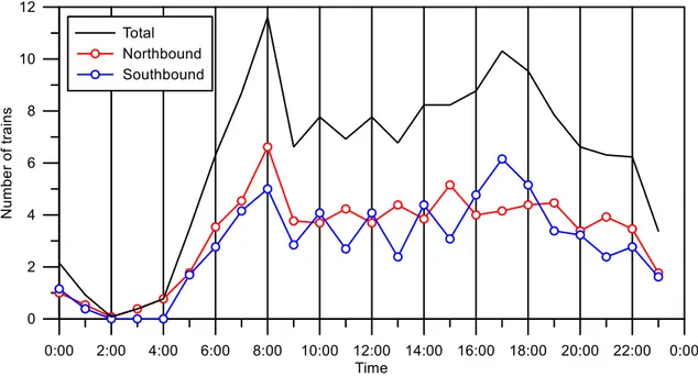
The mean number of trains registered per hour during the measurements is shown in Figure 9. Traffic peaks are found in the morning and in late afternoon and a minimum during late night hours.

Figure 9. Mean number of trains per hour during the measurements at Arlanda C.

Using the national system LUPP for monitoring punctuality and disturbances train traffic in

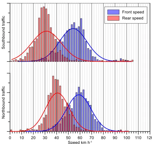
co-operation with Trafikverket (Anna Kryhl) it was possible to identify each train registered by the traffic measurements system. In Figure 10 the speed histograms for the registered train fronts and rears are shown. The northbound traffic has a slightly higher speed and a faster retardation than the southbound traffic when passing the traffic detection system. The reasons to this might be manifold. E.g., the configuration of the railroad approaching the platform might differ and affect the driving in the two directions. The placing of the traffic detection system in relation to the normal braking procedure might also cause an apparent difference.

In Figure 11, the calculated train lengths are shown. Obvious groupings can be seen that are similar in both southbound and northbound direction. Most trains are between 80 and 240 m long. From the frequency and lengths, it can be concluded that the high peak at around 105 m are single set commuter trains and the peak at 210 m double set commuter trains.

Figure 10. Speed histograms showing the front and rear speed of trains in south- and northbound directions.

3.1.2. Söderleden road tunnel

Figure 12 shows, as an example, the total number of vehicles recorded by the congestion charge portal divided into northbound and southbound traffic for the first week of the measurements. Between this portal and the measurement point inside the tunnel there is only one exit ca 420 meters from the main exit of vehicles from the road tunnel. How many vehicles that take this exit is not known, but likely 10% or less of the number passing the portal on the Johanneshovsbron. The northbound traffic peaks during the morning rush hour while the southbound peaks during the afternoon. During the weekend, no northbound morning rush hour peak is noticed, but traffic peaks at about noon. The southbound traffic peaks at about the same time as during Monday – Friday, but with lower traffic amounts.

Figure 12. Total traffic north and south passing the congestion portals at Johanneshovsbron during part of the measuring period (15 minutes time resolution).

Total daily mean traffic during the measurement period was around 53,000 vehicles per day during weekdays. However, it was also a variation with the traffic increasing during the week from Monday to Friday as seen in Figure 13. The total traffic northbound during weekday was about 27,500 vehicles per day compared to 25,500 southbound as presented in Figure 13. The average total traffic during weekends were 40,000 vehicles per day and the northbound traffic peaks earlier in the day than the southbound. The difference between the directions were smaller (around 1,000) during weekends compared to weekdays.

Figure 13. Total daily traffic north and south passing the congestion portals at Johanneshovsbron during the measuring period.

Different vehicle classes were measured during weekday daytime. The average diurnal variation for the traffic southbound is presented in Figure 14. Between 06:00 and 19:00 passed 76.2% of the total daily traffic. For the daytime traffic, 71.9% of the traffic was personal cars, 23.2% was light duty trucks, 3.7% was heavy duty trucks and 1.3% was busses. Both personal cars and light duty vehicles show a peak in the afternoon while the heavy-duty trucks show have a higher frequency during daytime and buses have maxima in the morning and late afternoon.

Figure 14. Mean daytime diurnal variation in number of vehicles for different classes when passing the congestion portals at Johanneshovsbron. Almost the same number of vehicles pass by the measurement station inside the tunnel.

Unfortunately, there are no traffic speed measurements available in the tunnel but the signed speed was 70 km/h.

The number of vehicles using studded tyres are counted manually at different streets and roads in Stockholm. No counting was made in the road tunnel but on Nynäsvägen which is the same road as Söderleden road tunnel, some 2 km south. Around 300 cars were counted on the 22 February and the studded tyres share on personal cars were 53% (Brydolf et al., 2013).

3.2.

Particle and NO

concentrations (TEOM, NO

, CPC)

3.2.1. Temporal patterns in the Arlanda C railroad tunnel and relation to traffic and

meteorology

Figure 15 shows NO and NOx concentrations as well as PM10 (TEOM) and particle number

concentration (CPC). During the first week of measurements, the high NO concentrations showed that exhaust was occasionally present in the tunnel, probably due to planned maintenance activities using diesel engines. These occasions were identified by high nitrogen oxide concentrations, when the ratio of particle number to nitrogen oxides was similar to published data on road traffic exhaust, i.e. around 1.5-2.4*1014 particles per gram of NOx (Janhäll and Hallquist, 2005). During the rest of the campaign, the nitrogen oxides were present in low concentrations and the ratio varied.

In the railroad tunnel the concentrations of nitrogen oxides are low compared to outdoor urban air, while the PM10 concentrations are extremely high and particle number concentrations are mainly in level with outdoor urban background air (SLB, 2014).

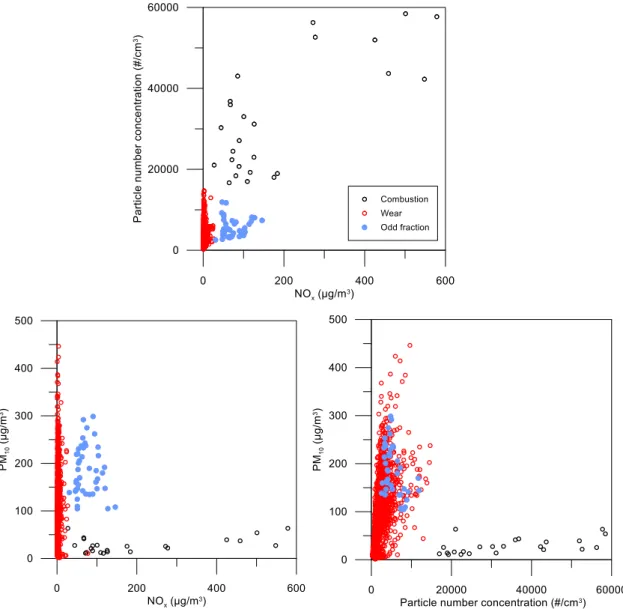
Figure 16. PM10 relations to NOx and particle number and particle number relation to NOx at Arlanda

C. Data has been classified based on some criteria as discussed in the text.

When all data is included in the scatterplots the correlations between pollutants are low at Arlanda C. Figure 16 shows scatterplots of particle concentration, both as mass and number, together with NOx concentration. The data has been divided into two main categories and an “odd fraction” of data, defined by a time period of high NO and low NO2 concentrations. Occasions with particle number concentrations above 15 000 / cm3 _{and NO}

x concentrations of above 1 µg/m3 was separated as being connected to influence of combustion particles. The PM10 concentrations are below about 75 µg/m3, but increasing linearly with increasing particle number (lower right in Figure 16). Occasions with lower particle number but PM10 ranging from 0 to almost 500 µg/m3 are considered as being connected to coarser wear particles. Plotting NOx to PM10 (lower left), shows that the data considered as

combustion-related show a similar trend as number concentration to PM10, but also reveals that some of the data considered as dominated by wear (PM10 above 100 µg/m3), also are connected to higher NOx concentrations (“odd fraction”). NO/NO2-data show that these data from the 31st of January have high NO concentrations, practically no NO2 and low particle number, why vehicle exhaust does not seem to be a likely source. A possible source to NO could be electrostatic discharges from the trains’ conductors. This is a process common during lightning in the atmosphere (e g., Bond et al., 2001), but it is unknown whether the dissipation energy formed is enough for this process to occur in the railroad tunnel.

Most of the vehicle exhaust was present during night-time and connected to maintenance vehicles, but for 31st _{of January, the source for NO with concentrations above 20 µg/m}3 _{is unknown. The PM}

10 concentrations are shown in green in Figure 17 for data without exhaust present and in yellow when concentrations of NOx were above 4 µg/m3. The relation to specific trains and vehicles are further investigated in chapter 3.3.1.

Figure 17. PM10 concentration at Arlanda C with the occasions with NOx above 4 µg/m3 marked as

yellow.

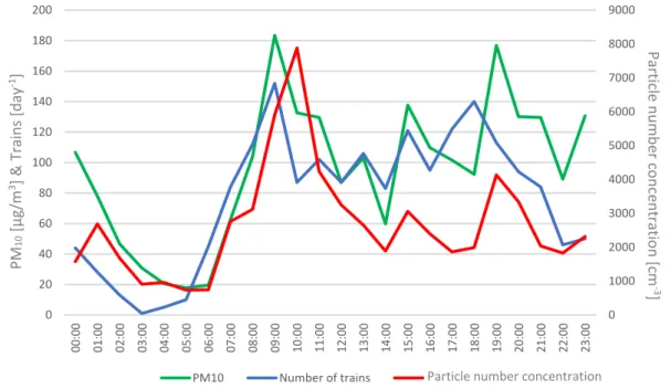
The diurnal variation of particle concentrations is shown in Figure 18, averaged over each hour of a day, where the blue line is traffic data from the last week of the campaign when no diesel exhaust emissions were detected. Particle concentrations reach minimum during early mornings just before morning traffic starts, while maximum concentration, averaged to around 200 µg/m3 _{or 7000 /cm}3_{, are} generally related to morning rush hours. After the morning peak the particle number decrease rapidly again only affected by the evening rush hour, while PM10 is high most of the day with rather similar concentration in the morning and evening peak.

Figure 18. Particle concentration averaged over a full day, one week without exhaust for the particle

0 50 100 150 200 250 300 350 400 13-02-01 12:00 13-02-02 12:00 13-02-03 12:00 13-02-04 12:00 13-02-05 12:00 13-02-06 12:00 13-02-07 12:00 13-02-08 12:00 13-02-09 12:00 13-02-10 12:00 13-02-11 11:00 PM 10 [µg/ m 3] PM10 PM10 - no exhaust 0 1000 2000 3000 4000 5000 6000 7000 8000 9000 0 20 40 60 80 100 120 140 160 180 200 00:00 01:00 02:00 03:00 04:00 05:00 06:00 07:00 08:00 09:00 10:00 11:00 12:00 13:00 14:00 15:00 16:00 17:00 18:00 19:00 20:00 21:00 22:00 23:00 Pa rticle n u m b er [p er cm 3] PM10 [µ g/m 3] & T ra in s [p er d ay ]

PM10 Number of trains Particle NumberParticle number concentration

Pa rticle n u m b er con ce n tra tio n [c m -3 ] PM 10 [ µ g/m 3] & T ra in s [da y -1]

Equally many train passes in the morning as in the evening peak hour, but the concentrations are much higher during the morning for particle number, while particle mass peaks are more similar. Both concentration peaks are delayed compared to the traffic peaks, even though the time difference is not possible to see, as even a small delay might move the particle concentration peak to be included in the next hour average.

The particles within the tunnel are probably related both to wear of rails and wheels etc., and to resuspension of the dust present in the tunnel. As wet grounds are known to reduce particle

resuspension, occasions of precipitation are shown together with PM10 concentrations in Figure 19. The precipitation data is corrected for snow where the data is purple. During rain events, the data is blue. During 6-8 of February, the PM10 concentrations seem to be reduced by the precipitation recorded while dryer periods have higher concentrations of PM10. This calls for a study of the impact of outdoor meteorological conditions like temperature and humidity, on the concentrations inside the tunnel. It seems that the outdoor conditions affect suspension of PM inside the tunnel. If all

concentrations are averaged over either the non-precipitation or the precipitation events, the concentration is 20% lower during precipitation events.

Figure 19. PM10 concentration and precipitation from the Arlanda meteorological station. PM10

during diesel contamination is given in yellow and precipitation corrected for snow is purple.

0 0,1 0,2 0,3 0,4 0,5 0,6 0,7 0,8 0,9 1 0 50 100 150 200 250 300 350 400 Prec ip ita tio n [m m /h r] PM10 [µ g/m 3]

3.2.2. Temporal patterns in the Söderleden road tunnel and relation to traffic and

meteorology

Nitrogen oxides are displayed together with particle number and mass concentrations in Figure 20, showing the high concentrations of nitrogen oxide in the road tunnel as compared to the previously described train tunnel. The nitrogen oxides have lower daytime concentrations during weekends, as five consecutive peaks are followed by two lower peaks due to lower weekend traffic. In addition, particle number is on average 20–30 times higher compared to the concentrations in the train tunnel. The high concentrations are present during a larger part of time. The PM10 concentrations are about three times as high as in the railroad tunnel, and very low in the first part of the campaign.

The low PM10 concentrations in the first part of the campaign coincides with high humidity outside the tunnel indicative of wet road surface conditions suppressing particle suspension due to traffic

turbulence in the tunnel, see Figure 21. Rain events in the area were recorded. The Söderleden road tunnel data are analysed together with meteorological data from Torkel Knutssonsgatan (www.slb.se), situated nearby the northern entrance of the tunnel.

Figure 20. NO and NO2, number concentration and PM10 in Söderleden road tunnel (15-minute mean

values). PM10 data was lost after 6th of March due to a tunnel washing occasion that flooded the

instrument inlets.

Figure 21. Traffic counts from bridge south of Söderleden road tunnel, particle concentrations and rain events causing humid conditions, defined as situations with vapour pressure deficit below 0.03.

The effect of humidity is visible as the first part of the campaign had wet conditions that later dried up, as shown in Figure 21. Events of vapour pressure deficit1 _{below 0.03 are marked as purple and the} effect on PM10 concentrations is shown. The effect of using relative humidity instead of VPD is not large, but as the focus here is on possible condensation of water, VPD is a better defined physical property. Particle number, on the other hand, follows the traffic in the tunnel relatively well. For pollution ratio analyses the five wet days during the campaign were compared to five dry days keeping the weekday constant to minimize the effect of weekend traffic on the result. The ratio dry/wet for PM10 was about six, while ratios for NO and particle number were close to one. The dry/wet ratio for NO2 was slightly higher than one, which might relate to nitrate chemistry, but that is merely a speculation.

The correlation between traffic and air pollutants is around 0.7–0.9 for all situations apart from PM10 during dry conditions, where the correlation is only 0.3. This shows that during dry conditions PM10 has a more complex relationship to traffic, likely to include fleet composition characteristics, such as ratio of heavy duty vehicles and time delay due to resuspension and deposition processes, whereas particle number and NOx are controlled by exhaust emissions.

1 _{VPD calculated from relative humidity and temperature according to} 1−𝑅𝐻

100 ∗ 0.6108 ∗ 𝑒 17,27∗𝑅𝐻 𝑇+237.3 0 50000 100000 150000 200000 250000 0 500 1000 1500 2000 2500 3000 Pa rticle n u m b er (p er cm 3) Tra ff ic cou n ts (p er h o u r) & PM10 (µg/m3 )

Figure 22. PM10 relations to NOx and particle number and particle number relation to NOx during the

wet (-2013-03-21) and the dry (2013-03-21-) periods.

Correlation between pollutants divided into wet and dry period are shown in Figure 22. A population of data during the wet period seems to belong to the dry period and vice versa, which shows that the actual dry and wet conditions are more detailed and separated in time than the simple division in periods made here.

In Figure 23, the variation of PM10 during the wet and the dry periods in connection to meteorology at rooftop height is shown. Meteorological parameters affect PM10 concentration, but the very scattered data in the plots indicate that the effects are likely to be subordinate to the occurrence of dry road surfaces when it comes to PM10 concentrations.

Figure 23. PM10 -concentrations during the wet and the dry periods and the relations to

meteorological parameters. Meteorology taken from rooftop measurements at Torkel Knutssonsgatan, ca 1 km from the northern tunnel opening.

Figure 24. Concentrations of NO and NO2 together with traffic counts in the southerly direction.

Figure 24 shows the nitrogen oxides together with traffic counts for south direction. NO clearly follows the traffic weekly variation with low weekend concentrations, while the weekend effect on NO2 is visible but smaller. The daily cycle differs between traffic and NO, as the peak is high for NO during morning and for traffic during afternoon, shown also in the diurnal variation (Figure 25). This could be due to influence from the other tunnel bore that has the traffic peak during the morning.

Figure 25. Diurnal variation in southbound traffic, NOx and NO during workdays, as an average

between the dry and the wet periods (thus referred to as “tot”). 0 500 1000 1500 2000 2500 3000 3500 4000 4500 5000 Tra ff ic cou n ts (p er h o u r) & N O an d N O2 (µ g/m 3)

Traffic north NO NO2

0 500 1000 1500 2000 2500 3000 3500 00:00 01:00 02:00 03:00 04:00 05: 00 06:00 07:00 08:00 09:00 10: 00 11:00 12:00 13:00 14:00 15:00 16:00 17:00 18: 00 19:00 20:00 21:00 22:00 23:00 Tr af fic so uth [#/hr] NO & NO x [µg /m 3]

Traffic south - tot NO-tot NOx - tot

Figure 26 Diurnal variation for traffic counts in the southbound direction, for workdays of the two different weeks and for weekends.

Figure 26 shows the traffic counts averaged over each hour of the workday divided into wet and dry period, and weekend, respectively. The traffic during the two weeks of dry and wet workdays is almost identical, while the weekends lack the morning peak.

The particle number concentration has one continuous peak between 07:00 and 17:00 for wet and dry conditions but ends slightly earlier during dry conditions (Figure 27, upper). The peak is higher for wet conditions even though traffic counts does not differ. During weekends, the peak is even smaller than for dry conditions and peaks slightly later in the day. PM10 during dry conditions peaks in the morning but falls off slightly again at lunch time, and another peak is formed during the early evening, still later than the traffic afternoon peak (Figure 27, lower). PM10 concentrations are similar for wet workday and weekend conditions, even though the night-time concentrations are higher during weekends.

0

500

1000

1500

2000

2500

3000

Figure 27 Diurnal variation for particle number concentration (upper) and particle mass (PM10)

concentrations (lower) for wet and dry conditions during working days and for weekends respectively.

The particle number concentration has one continuous peak between 07:00 and 17:00, while the PM10 peaks in the morning but falls off slightly again at lunch time. This might also be related to wetter conditions during afternoon. Varying meteorological conditions during this short period should have some impact on the results. Wet conditions increase particle number as compared to dry conditions, i.e. a smaller effect than on PM10 but in the opposite direction.

3.3.

Particle size distributions (APS, SMPS, ELPI)

Mean size distributions for the wet and the dry period in Söderleden road tunnel and the whole period for Arlanda C is shown in Figure 28. The mass size distribution for dry period in the road tunnel has a peak at about 4 µm while the distribution at wet conditions is bimodal with peaks at 3 and 0.7 µm. The Arlanda C distribution peaks at 2–3 µm.

At Arlanda C the mean number concentration is generally very low. An example of a short particle number peak can be seen in Figure 28, with a primary peak at 30 nm and a tendency for a secondary peak at 50 nm. 0 50000 100000 150000 200000 00 :0 0 02 :0 0 04 :0 0 06 :0 0 08 :0 0 10 :0 0 12: 00 14 :0 0 16 :0 0 18 :0 0 20 :0 0 22 :0 0 P article n u m b er co n centratio n [#/ cm 3 ]

Particle number concentration - wet Particle number concentration - dry Particle number concentration - weekend

0 100 200 300 400 500 600 700 800 00:00 01:00 02:00 03:00 04:00 05:00 06:00 07:00 08:00 09:00 10: 00 11:00 12:00 13: 00 14:00 15:00 16: 00 17:00 18:00 19: 00 20:00 21:00 22: 00 23:00 PM1 0 c oncen tr ation [µg /m3]

The particle size distributions of the Söderleden road tunnel in Figure 28 are averaged over the same time of day, but split into wet and dry periods, respectively, and show much higher concentrations of 3–4 µm particles during dry conditions, and slightly higher sub-micrometre mass concentrations. The distributions during both periods have a primary number peak at 20–30 nm and a secondary peak at about 100 nm. The wet period has lower concentration of most particle sizes, but also a slightly lower particle size in the peak (25–30 nm). The lower concentrations during wet conditions might be due to the fact that the data is from a Saturday as compared to the dry data sampled on a Monday.

Figure 28 Mean mass and number particle size distributions during wet and dry period in the Söderleden road tunnel and at Arlanda C.

Variations in size distributions over 24 h during wet and dry periods in Söderleden road tunnel can be seen in the examples presented in Figure 29 and Figure 30. Observe the differences in mass size distribution between dry and wet periods. The bimodal distribution of the coarse particles is obvious during the wet period, but the two modes do not necessarily coincide in time, pointing at different sources or processes affecting the concentrations. The wet period day showed in Figure 29 is a Saturday, with rather high traffic flows during the early hours (likely to be taxis, buses etc.) and a late morning rush hour starting at around 9. A rather distinct lunch hour minimum (13–15) can be seen in both the coarse fraction of the mass distribution and number distributions, while the finer fraction in the mass distribution does not display a similar minimum.

The number concentration distribution does not display obvious differences in wet and dry conditions while the mass size distribution has much higher concentrations and is coarser during dry conditions. The concentration is high also during night time, even though traffic is much lower. The concentration peaks also seem more isolated than during daytime, interpreted as suspension by single vehicles, likely to be heavy duty vehicles. For comparison, size distribution time series for a day at the railroad station Arlanda C is shown in Figure 30. The low traffic intensity compared to the road tunnel is reflected in the concentration peaks and the much lower number concentration stands out from the road tunnel data. A shift to a coarser background number distribution is seen at about 5 P.M. Number peaks associated with train passages does not seem to be affected by this shift, why it is likely to be related to an outdoor shift in air mass properties penetrating into the tunnel.

Figure 29. Time series of particle mass and number size distribution during a day with wet road

surface in Söderleden road tunnel.

Figure 30. Time series of particle mass and number size distribution during a day with dry road

Figure 31. Time series of particle mass and number size distribution Friday 1st of February 2013 at Arlanda C.

In Figure 32, the total particle mass concentration as a function of geometric mean particle size is shown for the two tunnel sites. The Söderleden road tunnel has two distinct data clusters, representing the initial wet period, with low PM10 concentrations and the final longer period with high PM10 concentrations. During the wet period the concentration is relatively low and the particle size range is wide from about 1.1–4 µm, with the highest concentrations when particle mean size is around 2–3 µm. During the night between the 19th _{and 20}th _{February between 19 PM to 6 AM, concentration and mean} particle size successively grow followed by a high variation in concentrations but within a smaller particle size span between 3–4 µm, indicating dominating contribution from road dust suspension. At Arlanda C the size/concentration plot resembles the road tunnel plot during the wet period.

Figure 32. Particle mass concentrations as a function of mass-weighted geometric mean particle size in the road and railroad tunnels. Dark blue is wet conditions in the Söderleden road tunnel. The other colours in the left graph represent different time periods while the tunnel dries up.

Figure 33: the road tunnel has about one order higher concentrations and a smaller size span than the railroad tunnel, likely reflecting more uniform exhaust related sources. A trend of decreasing

concentrations at higher mean diameter can be seen in both data sets.

Figure 33. Number concentration of ultrafine particles as a function of geometric mean particle size in the road and railroad tunnels. (Söderleden road tunnel in red and Arlanda C railroad tunnel in black.)

3.3.1. Detailed studies of train type (individual) effects at Arlanda

From data on time series of particle size distributions, trains related to peaks in mass size distributions of PM10 and number size distributions of ultrafine particles have been identified on individual level using the LUPP-system and traffic data collected during the measurements. The amount of data is voluminous and it has not been possible to analyse the whole dataset. However, in Figure 34 and Figure 35, two days of size distribution time series from APS and SMPS instruments are shown. On

initiate mass peaks of the coarse fraction detected by the APS and, in some cases, ultrafine number peaks detected by of the SMPS. It can also be seen that the arrival of the specific train set RC6 1419 three times during the day in Figure 34 results in similar mass peaks. RC6 1344 generates an obvious ultrafine peak, while RC6N 1388 and the “Long night train” only results in small ultrafine particle concentrations and “RC 1419” no ultrafine peaks at its three passages of the station. In Figure 35 the high ultrafine peak from a diesel driven maintenance vehicle is seen at 2 AM and exposes a slightly finer size distribution than the ultrafines from the electric trains during daytime. The shifts in peak size among mass size distributions suggest size differences between particles emitted from different trains. The only RC-train that passes twice (RC6 1342) generates similar mass size peaks, but the ultrafine particle generation is unclear. At 9 AM the train RC6P 1336 generates a comparably long-lived ultrafine peak. As can be seen in the two figures, there are some peaks that do not relate to RC-train passages.

How about other train types than RC? In opposite to the irregular arrival pattern of the regional trains, the X60 commuter trains arrive almost simultaneously from both directions every 30 minutes from 8 AM to 11 PM. The lack of periodically recurring mass- or number concentration peaks that coincide with the periodical commuter traffic indicates that these train sets are not major particle sources (Figure 34 - Figure 36). Also, the X50/X55 and the X40 train sets seldom coincide with particle peaks, but are harder to discern from the RC arrivals. Exceptions occur, like the most obvious ultrafine particle peak in Figure 35 which seems to be related X40 (or even X60) trains. One should note that there is a difference in braking time for the RC locomotive train sets compared to the other train types operating at Arlanda C. The braking time is longer and has more variability since it is also dependent on the number of wagons. Furthermore, the wagons can either have disc or block brakes. Also in terms of electrical braking the RC locomotive train sets differs since they are without electrical braking in contrast to the commuter trains operating at Arlanda C.

Figure 34. Mass-weighted particle aerodynamic size distributions from APS (right) and number-weighted particle mobility equivalent size distributions from SMPS (left) on 2013-02-03-04 from 1 AM to 1 AM with arrivals of RC-trains at arrows. Numbers relate to train individuals.

R

C

6N

13

88

R

C

6

14

19

R

C

6

13

44

R

C

6

14

15

Long

n

igh

t

tr

ain

Figure 35. Size distributions from APS (left) and SMPS (right) on 2013-02-05-06 from 1 AM to 1 AM with arrivals of RC-trains at arrows. Numbers relate to train individuals.

XXXX XXXX XXXX XXXX X6 0 X4 0 X5 0 & X55 RC

Figure 36. Size distributions from APS (left) and SMPS (right) on 2013-02-01. Numbers relate to train individuals. XXXX XXXX XXXX XXXX X6 0 X4 0 X5 0 & X55 RC