Simulation of diesel engines during transient conditions : Presentations : Summary of presentations made during the years 2001-2004

Full text

(1)VTI notat 16A-2005 Published 2005. www.vti.se/publications. Simulation of diesel engines during transient conditions Summary of presentations made during the years 2001–2004 Rolf Egnell.

(2)

(3) Preface VTI has on commission of VINNOVA and the Swedish Road Administration (VV) participated in COST 346: ”Emissions and fuel consumption from heavy duty vehicles”. In this commission VTI has engaged Lund Institute of Technology, Division of Combustion Engines. The research efforts at Lunds Institute of Technology have been executed by Rolf Egnell. This report, VTI notat 16A-2005 constitutes a summary of presentations at COST 346 meetings in 2001–2004. Project leader at VTI has been Ulf Hammarström. Contact persons: Carl Naumburg at VINNOVA and Håkan Johansson at VV. Gunilla Sjöberg, VTI, has performed the final revision of this document.. Förord På uppdrag av VINNOVA och Vägverket (VV) har VTI deltagit i COST 346: ”Emissions and fuel consumption from heavy duty vehicles”. Inom detta uppdrag har VTI anlitat Lunds Universitet, Institutionen för värme- och kraftteknik. Forskningsinsatserna vid Lunds Universitet inom COST 346 har genomförts av Rolf Egnell. Föreliggande VTI-notat utgör en delrapport inom uppdraget och utgör en sammanfattning av olika presentationer gjorda inom COST 346 under perioden 2001–2004. Projektledare vid VTI har varit Ulf Hammarström. Kontaktpersoner hos uppdragsgivarna har varit: Carl Naumburg (VINNOVA) och Håkan Johansson (VV). Gunilla Sjöberg, VTI, har svarat för slutredigering av dokumentet. Linköping september 2005. Ulf Hammarström. VTI notat 16A-2005.

(4) VTI notat 16A-2005.

(5) VTI notat 16A-2005. 1. Figure 1 This presentation is a summary of the work performed by Rolf Egnell at Lund Institute of Technology. The covered period of time is 2001– 2003. The objective of the work has been to develop methods to correct quasi stationary calculations of fuel consumption and emissions for transient effects.. Summary of transient correction work at Lund Institute of Technology. 2001 - 2003. COST 346.

(6) Figure 2. This work is financed by the Swedish National Road Administration and Vinnova. It is administrated by VTI (Ulf Hammarström). 2. VTI notat 16A-2005.

(7) VTI notat 16A-2005. 3. Figure 3. • Input data for engines and test-cycles. Generation of maps. • Observations concerning CO, HC and PM • Possible effects of changing boundary conditions • Quasi-static modeling. Effects of transients • Correction methods. Case wise - Stepwise • Conclusions. Outline of presentation.

(8) 4. VTI notat 16A-2005. Figure 4 Data from two heavy duty diesel engines, one MAN D 2866 LF 20 and one DAF XC 280 C1, were used in this study. The following slides show the MAN data.. MAN D 2866 LF 20. Engine maps based on static measurements.

(9) VTI notat 16A-2005. 5. Figure 5 MAN D 2866 LF 20 .This is the static map for fuel flow. The red dots is the load points for the measured input. The blue dots illustrates the load points (per second) for the ETC cycle. Most of the ETC points can be interpolated form measured data, but at some cases extrapolation is necessary. The lines in the figure show iso-fuel flow curves. The fuel flow is increasing almost linearly with torque and engine speed..

(10) 6. VTI notat 16A-2005. Figure 6 MAN D 2866 LF 20. This is a 3D illustration of the previous map..

(11) VTI notat 16A-2005. 7. Figure 7 This graph show the NOx-flow map. As can be seen the NOx-flow increases with torque. The dependence of speed is less clear and two maxima can be seen – one at about 1200 rpm and one at about 1800 rpm. It is likely that the valley between these speeds is a function of the optimization process for the cycle the engine is certified with (probably ECE R49 or ETC)..

(12) 8. VTI notat 16A-2005. Figure 8 MAN D 2866 LF 20. A 3D representation of the previous graph. The local minima at about 1400 rpm is easy to observe..

(13) VTI notat 16A-2005. 9. Figure 9 MAN D 2866 LF 20. The CO flow map is characterized by the steep increase at the top left portion of the load range. This is due to low lambdas in this region which in turn is due to low boost pressure..

(14) 10. VTI notat 16A-2005. Figure 10 MAN D 2866 LF 20. A 3D representation of the previous graph. The CO flow peek at low speed and high torque is dominating the CO flow landscape..

(15) VTI notat 16A-2005. 11. Figure 11 The HC flow map is characterized by the steep increase at the right portion of the speed range. This is probably due to over-leaning, which means that the a portion of the fuel is mixed with air to such a degree that the mixture becomes to lean to promote combustion. Another explanation could be that the air excess is so high that the temperature of the expanding gas is to low to support late oxidation of unburned fuel. The high air excess is caused by the performance of the turbo-charger at high engine speeds..

(16) 12. VTI notat 16A-2005. Figure 12 MAN D 2866 LF 20. A 3D representation of the previous graph. The maxima of HC-flow at high engine speeds is clearly seen..

(17) Lack of static data!. Figure 13 MAN D 2866 LF 20. This slide show the PM map. PM is a abbreviation for Particulate Matter. No measured data at negative torques were available when creating this map. This makes PM calculations more uncertain than for the other emissions. The general trend is that PM emissions increase at the higher loads at low speeds and high speeds. The increase at low speeds resembles the behavior as for CO. The reason for both cases is low oxygen concentration due to low boost pressure. A pronounced minimum is found at very low loads at the lowest portion of the speed range. The increase at higher speeds and loads could be connected to the higher HC emissions in this region. Condensed hydrocarbon on the surface of soot particles increases the mass of the particle.. VTI notat 16A-2005. 13.

(18) 14. VTI notat 16A-2005. Figure 14 MAN D 2866 LF 20. A 3D representation of the previous graph. Please notice the peek at low speeds and high torques and compare this slide with slide 10. The most likely cause of the peek is low lambda due to low boost pressure..

(19) VTI notat 16A-2005. 15. Figure 15 The results of quasi-stationary calculations are, to a great extent, depending on the interpolation technique used. The maps shown above were created using linear interpolation. Four of the following six pictures show maps generated with other techniques found in the Matlab library.. Interpolation techniques.

(20) 16. VTI notat 16A-2005. Figure 16 MAN D 2866 LF 20. Emission Index (g/kg fuel) PM map generated with linear interpolation. This is the same interpolation method as was used to generate the proceeding maps..

(21) VTI notat 16A-2005. 17. Figure 17 MAN D 2866 LF 20. Emission Index (g/kg fuel) PM map generated with Cubic interpolation..

(22) 18. VTI notat 16A-2005. Figure 18 MAN D 2866 LF 20. Emission Index (g/kg fuel) PM map generated with V4 interpolation..

(23) VTI notat 16A-2005. 19. - Triangle-. The 'cubic' and 'v4‘ methods produce smooth surfaces while 'linear' and 'nearest' have discontinuities in the first and zero-th derivative respectively. All the methods except 'v4' are based on a Delaunay triangulation of the data.. Figure 19 MAN D 2866 LF 20. Emission Index (g/kg fuel) PM map generated with linear interpolation. 'linear' based linear interpolation..

(24) 20. VTI notat 16A-2005. Figure 20 MAN D 2866 LF 20. Emission Index (g/kg fuel) PM map generated with Cubic interpolation. 'cubic' - Trianglebased cubic interpolation. The 'cubic' and 'v4‘ methods produce smooth surfaces while 'linear' and 'nearest' have discontinuities in the first and zero-th derivative respectively. All the methods except 'v4' are based on a Delaunay triangulation of the data..

(25) VTI notat 16A-2005. 21. Figure 21 MAN D 2866 LF 20. Emission Index (g/kg fuel) PM map generated with V4 interpolation. 'v4' - MATLAB 4 griddata method. The 'cubic' and 'v4‘ methods produce smooth surfaces while 'linear' and 'nearest' have discontinuities in the first and zero-th derivative respectively. All the methods except 'v4' are based on a Delaunay triangulation of the data. The V4 method gives the less detailed maps, but is more capable of extrapolation as can be seen when comparing the map areas in Figures 19 – 21..

(26) 22. VTI notat 16A-2005. [g/kWh]. HC 0.18 (1.39) 0.25 0.25 0.22. PM 0.16 (0.56) 0.09 0.08 0.09. Figure 22 MAN D 2866 LF 20. Calculations were performed with maps generated with all three methods. The results are shown in this table. Best overall results were achieved with the linear method although the V4 method come closest when calculating the fuel consumption. NOx emissions and fuel consumption are very well predicted with quasi stationary calculations, while CO and PM are under predicted and HC over predicted. The red numbers in brackets show the ratio calculated (linear)/measured.. Fuel and NOx well predicted Î Start of injection kept constant CO and Soot under-predicted. HC over-predicted. Measured Linear Cubic V4 (Matlab). FUEL NOx CO 213 10 1.15 (0.95) (0.98) (0.39) 203 9.8 0.45 202 9.7 0.43 217 11.1 0.43. ETC cycle. MAN-data.. Quasi static engine simulations. Different interpolation methods..

(27) VTI notat 16A-2005. 23. Figure 23 Data from two heavy duty diesel engines one MAN D 2866 LF 20 and one DAF XC 280 C1 were used in the study. The following slides show the DAF data.. DAF XC 280 C1. Engine maps based on static measurements.

(28) 24. VTI notat 16A-2005. Figure 24 DAF XC 280 C1. PM map. Linear interpolation. The peek value is found at high speed in contrast to the MAN engine. See also Figures 13 ,14, 31 and 32. Very few input data points (red dots). The reason that no peek is found at low speed and high torque, as was the case with the MAN engine, could be a better choice of turbo for the DAF engine..

(29) VTI notat 16A-2005. 25. Figure 25 DAF XC 280 C1. The CO map for the DAF engine resembles the CO map for the MAN engine. The maximum flows are achieved at low speed and high torque.See Figures 9, 31 and 32..

(30) 26. VTI notat 16A-2005. Figure 26 DAF XC 280 C1. The NOx map for the DAF engine resembles the NOx map of the MAN engine with respect to the influence of torque. However, the influence of speed is different. The DAF engine has two valleys while the MAN has one. See Figures 7, 31 and 32..

(31) VTI notat 16A-2005. 27. Figure 27 DAF XC 280 C1. The HC map for the DAF engine is completely different the HC map of the MAN engine. The DAF engine has two maxima – one at 1200 rpm max torque and one at about 1500 rpm 1000 Nm. These maxima are, however, based on very few input data and is thus very uncertain. See also Figures 11, 31 and 32..

(32) 28. VTI notat 16A-2005. Figure 28 DAF XC 280 C1. The Fuel flow map for the DAF engine resembles the Fuel flow map for the MAN engine. The flow is increasing with speed and torque. See Figures 5, 31 and 32..

(33) VTI notat 16A-2005. 29. Figure 29 DAF XC 280 C1. The lambda landscape of the DAF engine is shown in this slide. As can be seen the lowest lambda values are found in the upper right corner of the map. This is also the location of high CO emissions. The reason for to low lambda values at this region is the low boost pressure as can be seen in the next slide. The lambda value is increasing with the decrease of load. This is due to the unthrottled operation of the diesel engine..

(34) 30. VTI notat 16A-2005. Figure 30 DAF XC 280 C1. The Boost pressure landscape of the DAF engine is shown in this slide. As can be seen the boost pressure increases with speed, i.e. flow. The lowest boost pressures at maximum torque is found at the lowest engine speed. In order to maintain high torque in this region of the map, the fuel delivery per stroke has to be high despite the lower air supply. This explains to low lambda and the high CO and PM emissions in the MAN case..

(35) VTI notat 16A-2005. 31. Figure 31 DAF XC 280 C1. This is a summary slide for the DAF engine. It should be compared with the next slide which shows the same graphs for the MAN engine. A comparison show similarities between the two engines with respect to fuel flow, CO emissions and to some degree NOx-emissions. While the HC- and PM landscapes are different..

(36) 32. VTI notat 16A-2005. Figure 32 MAN D 2866 LF 20. This is a summary slide for the MAN engine. It should be compared with the slide above which shows the same graphs for the DAF engine. A comparison show similarities between the two engines with respect to fuel flow, CO emissions and to some degree NOx-emissions. While the HC- and PM landscapes are different..

(37) VTI notat 16A-2005. 33. Figure 33 The test cycles used in this study, 26 cycles all together, consist of established test cycles and vehicles cycles measured on the road and converted to engine cycles.. Test cycles.

(38) 34. VTI notat 16A-2005. Figure 34 This slide show the average power of the test cycles. The blue bars show the average value of all positive powers (sampled with 1 Hz). The red bars show the average value of all powers. The difference between the bars gives an idea of the degree of engine breaking. The first bars from the left represents the ETC cycle.. Transient testcycles.

(39) VTI notat 16A-2005. 35. Figure 35. Observations concerning CO, HC and PM.

(40) 36. VTI notat 16A-2005. Figure 36 This figure show Emission Index [g/kg fuel] for CO vs. the lambda value. All static input data where lambda is less than 6 are used in the figure. The figure show that CO for both test engines increases with decreasing and increasing lambda. The minimum is achieved at about lambda 2. When reducing lambda from this value the combustion will take place with too little air excess which gives higher CO emissions. When increasing lambda the combustion gas temperature becomes to low to promote oxidation of CO during the expansion stroke. This results in increased emissions.. MAN.

(41) VTI notat 16A-2005. 37. Figure 37 This figure show Emissions Index for PM vs. lambda. The general trend is that EIPM increases with increasing lambda. However it is very likely that EIPM also increases with decreasing lambda although that can not be seen in the figure because of lack of measurements at low enough lambdas. The reason for the observed and anticipated trends is air shortage on the “rich leg”, and too low exhaust temperature at the “lean leg”..

(42) 38. VTI notat 16A-2005. Figure 38 This figure show Emissions Index for HC vs. lambda. The general trend is that EIHC increases with increasing lambda. However it is very likely that EIHC also increases with decreasing lambda although that can not be seen in the figure because of lack of measurements at low enough lambdas. The reason for the observed and anticipated trends is air shortage on the “rich leg” and too low exhaust temperature at the “lean leg”, i.e. the same trends as was observed for CO and anticipated for PM.. MAN.

(43) VTI notat 16A-2005. 39. Down Down Up or Down Up or Down Up or Down. Lambda Up Up Down Down Down. T inlet. Up Down Down Down. Up Down Up Up Up. T walls Reciduals. Up Down Down Down. T ime Down Up Down Down Down. Down Up Down Down Down. Start of inj. Inj. Pressure. Figure 39 This table summarizes some ideas of what could be expected when changing the boundary conditions for combustion. Thus reducing lambda would possibly increase the fuel consumption due to increased combustion duration and reduced combustion efficiency. This statement is probably correct for high loads, but may not be valid for low loads. At high loads a major decrease of lambda would result in increased emissions of CO, HC and PM.. Fuel consumption NOx CO HC PM. Increasing/advancing:. Possible effects of changing boundary conditions.

(44) 40. VTI notat 16A-2005. Figure 40. Quasi-static modeling. Effects of transients.

(45) VTI notat 16A-2005. 41. Figure 41 This figure show the ratio between the Quasi-Stationary (QS) calculated accumulated fuel consumption and emissions and their measured counterparts. As can be seen QS calculations give very good results for fuel consumption and NOx-emissions, while CO and PM are under-predicted and HC over-predicted. This conclusion is valid for both engines, although only ETC data is available for the MAN engine. The two green arrows indicates the test cycles for which QS calculation gives the best results for CO and PM (cycle 4) and the worse (cycle 18) respectively.. MAN.

(46) 42. VTI notat 16A-2005. Figure 42 Although there are a considerable spread among the data, there seem to be a correlation between the ratios for CO, PM and HC – they all increase and decrease at the same time. As the ratio of CO and PM are constantly lower than 1 an increase means that the calculated value approaches the measured. The case is the opposite for HC where an increase means the calculated value deviates more from the measured..

(47) VTI notat 16A-2005. 43. Figure 43 This slide show the relation between the CO ratio and the PM ratio. For all cycles but one, the PM ratio is higher than the CO ratio. This means that the deviation between the QS calculated and the measured value is less for PM than for CO. The theory, so far, is that the reason why CO and PM are underestimated with QS calculation is that, due to the transient behavior of the turbocharger, the lambda value at the higher loads during increasing power is less than at stationary conditions. When the actual lambda value passes a lower limit the emissions of CO and PM increases rapidly. The reason why CO and PM acts somewhat differently is probably that the lower lambda limit is lower for PM than for CO..

(48) 44. VTI notat 16A-2005. Figure 44 This figure show measured and QS calculated CO flow vs. Time for cycle 4, i.e. the cycle were the QS calculated CO emissions come closest the measured. See figure 41. As can be seen the deviation between the two curves are considerable at some rather rare occasions. During most of the cycle the calculated and the measured flows are fairly close..

(49) VTI notat 16A-2005. 45. Figure 45 In opposite to the previous slide this slide show that the measured CO flow is considerably higher than the calculated at numerous occasions during the cycle. This is cycle 18, i.e. the one that gave the worst agreement between QS calculated and measured CO flows. See figure 41. It is interesting to notice that the measured flow deviates from the calculated as distinct peeks and not continuously over longer periods of frequents transients. According to the preliminary theory, this indicate that the duration of low lambda is rather short..

(50) 46. VTI notat 16A-2005. Figure 46 This slide show a close up of a section of cycle 26. The upper figure shows measured and QS calculated CO flow, while the lower show QS calculated and measured lambda. The lower figure shows clearly that measured (dynamic lambda) is considerably lower the QS calculated. The measured CO peaks occurs when the dynamic lambda becomes less than about 2. This was also noticed when looking at the static CO measurements. See figure 36..

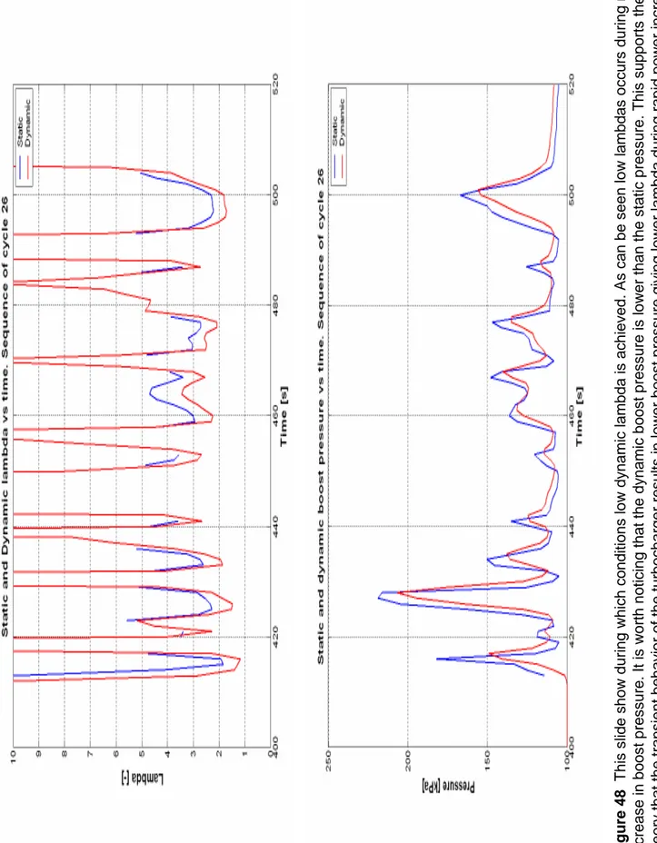
(51) VTI notat 16A-2005. 47. Figure 47 This slide show during which conditions low dynamic lambda is achieved. As can be seen low lambdas occurs at high fuel flows during rapid flow changes..

(52) 48. VTI notat 16A-2005. Figure 48 This slide show during which conditions low dynamic lambda is achieved. As can be seen low lambdas occurs during rapid increase in boost pressure. It is worth noticing that the dynamic boost pressure is lower than the static pressure. This supports the theory that the transient behavior of the turbocharger results in lower boost pressure giving lower lambda during rapid power increase..

(53) VTI notat 16A-2005. 49. Figure 49 This figure show that rapid changes of torque correlate stronger to lambda variation than engine speed changes..

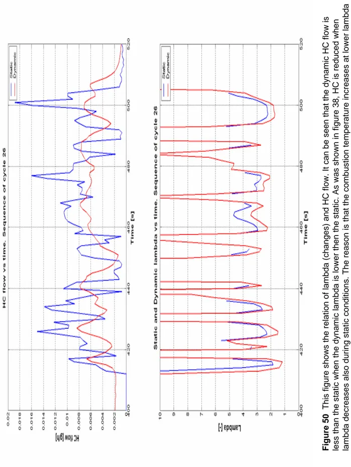
(54) 50. VTI notat 16A-2005. Figure 50 This figure shows the relation of lambda (changes) and HC flow. It can be seen that the dynamic HC flow is less than the static when the dynamic lambda is lower then the static. As was shown in figure 38, HC is reduced when lambda decreases also during static conditions. The reason is that the combustion temperature increases at lower lambda resulting in more complete combustion of the fuel. On the other hand the amount of CO and PM increases. Thus the behavior of CO, PM and HC supports the theory that rapid increases of load (torque) led to a reduction of lambda, due to the insufficient response of the turbocharger, which gives a reduction of HC but an increase of CO and PM..

(55) VTI notat 16A-2005. 51. Figure 51 The idea behind this figure is to check whether the dynamic exhaust temperature during dynamic conditions is higher than during static conditions. If that is the case, the theory of higher combustion temperature due to lower lambda during transients would be supported. The lower figure show, however, that the dynamic temperature varies less and reach lower levels than the calculated static temperature. The reason is probably the thermal inertia of the thermocouple rather than actual differences in the temperatures of the exhaust gas..

(56) 52. VTI notat 16A-2005. Figure 52 In this slide the dynamic (measured) lambda is plotted vs. the QS calculated lambda for every second of a light load cycle. As can be seen the bulk of the dots fall below the red 1:1 line. This means that at most conditions the dynamic lambda is less than the QS calculated..

(57) VTI notat 16A-2005. 53. Figure 53 In this slide the dynamic (measured) boost is plotted vs. the QS calculated boost for every second of a light load cycle. As can be seen the bulk of the dots fall below the red 1:1 line at boost pressures above 120 Pa. This means that at most high load conditions, the boost is less than the QS calculated. The lower dynamic boost pressure is the reason for the lower dynamic lambda which is in agreement with the, now strongly supported, theory saying the transient behavior of the turbocharger is the main cause to the under prediction of CO and PM and the over prediction of HC..

(58) 54. VTI notat 16A-2005. Figure 54 This is the same plot as shown in figure 52, but the average load of the test cycle is higher. The trend is the same at higher loads. i.e. lower lambdas, the dynamic lambda is less than the QS calculated static lambda..

(59) VTI notat 16A-2005. 55. Figure 55 This is the same plot as shown in figure 53, but the average load of the test cycle is higher. The trend is the same at higher loads. i.e. higher boost pressures, the dynamic pressure is less than the QS calculated static pressure. At very low loads (pressures) the dynamic pressure is higher the calculated static. This indicates the inertia of the turbocharger keeps the boost pressure up longer than calculated static pressure after a load reduction..

(60) 56. VTI notat 16A-2005. data are discussed.. Figure 56 In the following slides, different approaches to correct accumulated QS calculated. Correction of accumulated data Case wise correction. Correction methods.

(61) VTI notat 16A-2005. 57. Figure 57 In this figure the ratios of fuel consumption and emissions are plotted against the relative mean power of the test cycle. As can be seen there is a trend that the ratios approaches 1 for fuel flow (red line), NOx (blue line), CO (pink line) and PM (black line) as the relative mean power increases. The trend is the opposite for HC. As the relative mean power increases there is less “room” for load changes. Assume that the relative mean power was the same as the maximum power, this would tell that the engine is running on maximum power over the entire cycle and no variation of the load is possible. Thus, a higher relative mean power could indicate a less transient cycle. Less transients could explain the behavior of all ratios but the HC ratio in the figure..

(62) 58. VTI notat 16A-2005. Figure 58 In this figure the ratios of fuel consumption and emissions are plotted against the relative mean torque of the test cycle. As can be seen there is a trend that the ratios approaches 1 for fuel flow (red line), NOx (blue line), CO (pink line) and PM (black line) as the relative mean torque increases. The trend is the opposite for HC. As the relative mean torque increases there is less “room” for load changes. Please see the discussion on the previous slide. The scatter seem to be less when using the relative mean torque instead of the relative mean power..

(63) VTI notat 16A-2005. 59. Figure 59 In this figure the ratios of fuel consumption and emissions are plotted against the relative mean speed of the test cycle. As can be seen there is a trend that the ratios approaches 1 for fuel flow (red line), NOx (blue line), CO (pink line) and PM (black line) as the relative mean speed increases. The trend is the opposite for HC. As the relative mean speed increases there is less “room” for load changes. Please see the discussion on the previous slide..

(64) 60. VTI notat 16A-2005. Figure 60 This figure shows an attempt to use the inverse of the trend lines (derived by least square fit) to correct the QS calculated fuel data. As can be seen the maximum deviation from 1 is reduced from +2%/-6% to +3%/-2%. The best base for correction is the relative mean torque..

(65) VTI notat 16A-2005. 61. Figure 61 This figure shows an attempt to use the inverse of the trend lines (derived by least square fit) to correct the QS calculated NOx data. As can be seen the maximum deviation from 1 is reduced from +9%/0% to +5%/-4%. Equal results are achieved with all three correction bases..

(66) 62. VTI notat 16A-2005. Figure 62 This figure shows an attempt to use the inverse of the trend lines (derived by least square fit) to correct the QS calculated CO data. As can be seen the level of the ratios is increased but the deviation from 1 is still unacceptable..

(67) VTI notat 16A-2005. 63. Figure 63 This figure shows an attempt to use the inverse of the trend lines (derived by least square fit) to correct the QS calculated PM data. As can be seen the level of the ratios is increased but the deviation from 1 is still unacceptable..

(68) 64. VTI notat 16A-2005. Figure 64 This figure shows an attempt to use the inverse of the trend lines (derived by least square fit) to correct the QS calculated HC data. As can be seen a fairly good correction is achieved when using the relative mean torque as base..

(69) Correction based on the degree of transience. Figure 65 In the following slides an attempt the characterize a cycle be it degree of transience is presented. The idea is to use the inverse degree of transience to correct the QS calculated emissions. Only CO emissions was studied. Input is the QS calculated stepwise fuel flow of the cycle in question.. • The emission input to this model is accumulated data for a given engine running at different test cycles. • The relation between the QS CO ratio (calculated/measure) and the occurrence frequency of transients is used as input for correction.. VTI notat 16A-2005. 65.

(70) 66. K4. Second order curve fit. QS CO ratio vs transient frequency. K1. K3. Test cycle mean power. CORATIO_CORR=0.55*((300./MKW).^0.4).*CORATIO./(p(1)*FRACTION.^2+p(2)*FRACTION+p(3));. K2. pgradfuel=gradient(Sfuel); all=size(pgradfuel,2); pos=find(pgradfuel>1.55); select=size(pos,2); fraction=select/all; FRACTION=[FRACTION fraction];. MATLAB Algorithm. Figure 66 The transience methods includes 4 fitting parameters, K1 – K4. The degree of transience is defined by the frequency of fuel flow derivatives higher than K1. In this study the actual derivative is used, i.e. [g/s2). In order to generalize the method it is better to use a relative fuel flow derivative. The maximum power of the engine could probably be used giving K1 the dimension g/s2 kW. As can be seen in the next slide the CO ratio correlates fairly well with the frequency and a second order curve is used in the calculations. K1 has to fitted to minimize the spread. In the correction equation shown above, the CO ratio for the actual cycle is divided with the CO ratio achieved with the CO ratio derived from the curve fit. This step only gives an acceptable correction, but it was found that multiplying the result with the inverse of the relative power of cycle in question raised to a fitted exponent gave a better result. The rational for using the relative power in the equation is that a high relative power, i.e. a high fuel flow, indicates a less impact on the CO emissions of a given change of the fuel flow. If the method should be further developed is probably better to include the relative power or the maximum fuel flow when defining K1. K3 is the maximim power of the engine K4 is the fitted exponent K2 is the fitting parameter to compensate for the size of the power term.. VTI notat 16A-2005.

(71) VTI notat 16A-2005. 67. Figure 67 This figure shows the CO ratio vs. the frequency of fuel flow derivatives higher than 1.5 g/s2 . The red curve illustrate a second order least square curve fit..

(72) 68. VTI notat 16A-2005. Figure 68 This slide show the result of using the Transience Case Wise Correction method on CO. The accuracy of the method is about +/-20%.. Tuning cycle.

(73) VTI notat 16A-2005. 69. Figure 69 This slide show the result of using the Transience Case Wise Correction method on CO. All parameters, i.e. K1 – K4 and P(1) – P(3) is adapted by using the statistical program package SPSS..

(74) 70. VTI notat 16A-2005. Figure 70 With stepwise correction is meant that the QS calculated flow is corrected at every time step.. The impact of transients. Stepwise correction.

(75) VTI notat 16A-2005. 71. CO flow vs time. Calculated and measured data. DAF XC 280 C1. Sequence of Cycle 18 (ST0720A). Figure 71 This slide show a portion of cycle 18. The red curve is the measured CO flow and the blue curve is the corresponding QS calculated curve. The numbers indicate at what time step (s) the peak values are achieved.. CO flow [g/s].

(76) 72. VTI notat 16A-2005. Figure 72 This slide show the trajectory of the portion of the test cycle in the torque – speed domain. The numbers indicate the time step of the peaks in the small figure. It can be seen that the peak occur after a rapid increase in torque. The torque gradient is typically 1000 Nm/s from low load. This load change is characteristic for “full throttle” from idle. As can be seen the change of static CO flow is much less than measured..

(77) VTI notat 16A-2005. 73. Figure 73 This figure shows the trajectory added to the static lambda map. As can be seen the lowest static lambda value is about 2, which should not result in a the high CO flows measured. It is obvious that the dynamic lambda is less then the static..

(78) 74. VTI notat 16A-2005. Figure 74 Two parts of cycle 4 had been used to study the transient behavior of CO as a function of torque increase. The first part consists of time steps 165 – 170 as shown in the figure above. During this interval no transient deviation from QS calculated CO flow is noticed.. 165 - 170.

(79) VTI notat 16A-2005. 75. Figure 75 The torque increase in the time sequence 165 – 170 is about 70 Nm/s and starting from a fairly high torque level. In this figure this change is shown in the static CO map..

(80) 76. VTI notat 16A-2005. Figure 76 The torque change in the time sequence 165 – 170 is about 70 Nm/s. In this figure this change is shown in the static lambda map. As can be seen the torque change takes place at a region with lambda values above 3, which means that even if the dynamic lambda would become slightly less there would not be a noticeable increase in the CO flow..

(81) VTI notat 16A-2005. 77. Figure 77 Two parts of cycle 4 had been used to study the transient behavior of CO as a function of torque increase. The second part consists of time steps 125 – 130 as shown in the figure above. During this interval major transient deviation from QS calculated CO flow is noticed. 125 - 130.

(82) 78. VTI notat 16A-2005. Figure 78 The torque increase in the time sequence 125 – 130 is about 500 Nm/s and starting from a low torque level. In this figure this change is shown in the static CO map..

(83) VTI notat 16A-2005. 79. Figure 79 The torque change in the time sequence 125 – 127 is about 500 Nm/s starting from a very low torque (about -100 Nm). In this figure this change is shown in the static lambda map. As can be seen the initial torque change takes place at a region with lambda values above 4. Despite the high static lambda value the measured CO flow indicate a lambda value below 2. It is obvious that the turbo lag increases if the load increase starts from a very low torque level. In this case at a negative torque indicating engine breaking..

(84) 80. VTI notat 16A-2005. Figure 80 This figure show the rapid torque increase during time step 125 – 127 in the PM map..

(85) VTI notat 16A-2005. 81. Figure 81 Two methods of stepwise correction has been studied. One is based on a mechanistic approach and the other is based on identification of a correction factor.. • A mechanistic approach – the delay model • Correction factor identification. Stepwise correction.

(86) 82. VTI notat 16A-2005. Figure 82. The Delay Model. A mechanistic approach.

(87) VTI notat 16A-2005. 83. Tt2 Mdot_exh. When the load is reduced by decreasing the fuel flow the turbocharger delivers a higher air flow due to inertia of the rotating parts. The speed of turbocharger do not adopt to the lower load immediately and the lambda becomes higher than during static conditions.. Figure 83 The delay model could also be called a turbo-lag model because it tries to capture the behavior of the turbocharger during a torque increase. As the power of a diesel engine is controlled by the amount of fuel injected into the cylinders an increase of the load takes place by increasing this amount. At the time of a increase the air flow is still dimensioned for the previous lower fuel flow which means that lambda is reduced. The increased fuel flow (and lowered lambda) increase the exhaust temperature (Tt1 in the figure) which increases the enthalpy of the exhaust. The increased enthalpy make the turbine accelerate and thus the speed of the compressor increases. As the speed of the compressor increases, the air flow increases and after a certain time the air flow again matches the fuel flow. During the process of adapting the airflow to the new fuel flow lambda is constantly below the lambda at the corresponding static load.. Power balance at static conditions. Mdot_air x Cp_air x (Tc2 – Tc1) = Mdot_exh x Cp_exh x (Tt1-Tt2). Tc1 Mdot_air. Tc2. Tt1. The turbocharger.

(88) 84. VTI notat 16A-2005. The figure show the relation between measured static Emission Index CO and lambda. This is the same figure as shown above (figure 36). By a function adopted to these data points a relation between the CO emissions at different lambda values, one static and one transient, could be calculated as illustrated I the figure. Thus, the challenge become to estimate the transient lambda. How this is done is shown in the next slide.. Figure 84 So far the delay model has only been developed for CO correction. The reason for this is that no time step resolved measurements for PM were available. The idea was to use the relation between the CO ratio and the PM ratio to, in a second step, correct the calculated PM..

(89) VTI notat 16A-2005. 85. The plan for developing the Delay Model included firstly: identification of the delay (τ) necessary to correct the CO emissions at every time step. And secondly: finding an equation that was capable of calculating the delay time at every time step. Due to reasons discussed in figure 87 it was not possible to identify the delay time for the many of the time steps responsible for most of the transient CO emissions.. Figure 85 The Delay Model got its name because it is assumed that the airflow is constantly lagging the fuel flow. The method is illustrated in the figure above. The fuel flow and lambdas at times t (426) and t-tstep is obtained from the QS calculations. By using the fuel flow and lambda at time t and t-tstep, the static air flows at the corresponding times could be calculated. By interpolation within the time step the air flow at time t-τ could be estimated. τ is the delay time. By using the fuel flow at time t and the air flow at time t-τ, the “transient” lambda at time t could be calculated. The static and transient lambdas are used to calculate the CO correction factor as shown I figure 84. The delay time do not have to be equal or less than the time step, but that limitation is introduced in the figure for pedagogic reasons..

(90) 86. VTI notat 16A-2005. Figure 86. Available input.

(91) VTI notat 16A-2005. 87. Figure 87 This figure show the trajectory of cycle 18. As can be seen many of the steep load torque increases starts a very low and even at negative torques. This is illustrated by the numerous almost vertical sequences at the right portion of the graph. This behavior entailed major problems to the Delay Model. The reason for this is that the models rests on the assumption that static data is available before a transient takes place. It was found that that was not the case for transients starting at very low or negative loads. The reason is that too few measured static data points are available at this regions. The map generator used, Matlab linear interpolation, could not solve the problem if the data points were to sparse or if extrapolation was needed..

(92) 88. VTI notat 16A-2005. Figure 88. All data. Input Statistics.

(93) 52 72 72 72 72 48 48 107 106 34 98 30. Accum. Meas. / Bag mass (all data) Accum. Meas. / Bag mass. Reduced input based on aviliable QS data Accum. Calc. / Bag mass (all avaliable QS data). Accum. Meas. / Bag mass. Reduced input (Common with SLAMBDA excl. NaN inf) Accum. Calc. / Bag mass Reduced input (Common with SLAMBDA excl. NaN and Inf). [%]. All. Lambda Fuel NOx CO HC PM Boost. Usable QS data. Input map generation Available CO data with MATLAB. The accumulated QS calculated CO mass represent only 34% of the bag mass, which illustrates the average underestimation of CO by QS calculation.. If only summarizing the measured CO flows at time steps where a QS calculated CO value are available the value exceeds the bag value with 6%. This show that the missing 28% of the static CO data represent less than 1% of the total accumulated CO mass.. However, an analysis show that the available static CO data represent a major portion of the total flow. This is shown in the lower part of the table above. If all step wise measured flows are compared with the total amount of CO calculated from the bag values the ratio is 1.07, which means that the accumulated on line measured CO flows exceeds the measured bag mass with 7%.. As can be seen in the table at 52% of the time steps I was possible to calculate a static lambda value. For fuel, NOx, CO, and HC flow 72% of the time steps resulted in useful data. For PM an Boost the percentage were 48%. This situation is not satisfactory and measures has to be taken to improve the map generation.. Figure 89 All the test cycles included more than 18 000 time steps. The table above tells how big a portion of this time steps for which is was possible to calculate static map data. Missing data is detected as NaN (not a number) or Inf (infinity) and are caused by the shortcomings of the function “griddata” in Matlab.. VTI notat 16A-2005. This exercise show that it would be possible to calculate an accumulated CO mass by only using time steps where static data is available. The problem with the Delay time approach it in addition to data from these time steps needs data at time steps where the CO flow is insignificant for the total mass.. If only summarizing the calculated CO flows at time steps where a QS calculated lambda values are available the value correspond to 30% of bag mass.. If only summarizing the measured CO flows at time steps where a QS calculated lambda values are available the value correspond to 98% of bag mass This show that the missing 48% represent less than 8% of the total accumulated CO mass (98/107 = 0.92).. 89.

(94) 90. VTI notat 16A-2005. Figure 90 This figure shows the results from using the present version of the Delay model with identified delay times. The accuracy is about +-20% this figure could be improved a lot if CO data from more time steps could be included. In principle it should be possible to get a CO ratio of one for all cycles. When that is accomplished the next challenge would be to find a function that would be capable of estimating the delay time.. Identified delay times. Best results with the delay model.

(95) The Delay Model Conclusions. 91. Figure 91. • High potential, but needs detailed engine and turbocharger input. • Detailed static fuel flow, lambda, boost and emission maps covering the entire load range needed. Information from preceding steps needed. • The QS EICO – Lambda relation is probably not correct for all load points especially not for higher lambda values. • The assumption that the dynamic lambda can be calculated from the QS map are probably an oversimplification. • Not suitable for input generated within COST 346. VTI notat 16A-2005.

(96) Correction factor identification. Figure 92 This approach is strongly related the case wise correction based on the degree of transience presented above. The difference is that the correction is made at every time step and that a power related fuel flow derivative is used.. • Identification of the occurrence of transients • Step wise correction of QS CO data to transient emissions. 92. VTI notat 16A-2005.

(97) VTI notat 16A-2005. 93. %(13.33) Fixed correction factor during transients. corr(j)=k2;. Sco_corr(j)=Sco(j);. Figure 93 This is the Matlab algorithm used. The threshold fuel derivative k1 is fitted to 420 g/s2 kW. Where the power used is the maximum power of the engine. When the max power normalized fuel gradient is exceeding k1 the QS calculated CO flow is increased with the other fitting parameter k2 (13.33). The results of this correction is shown in the next slides.. end. end. else. Sco_corr(j)=corr(j)*Sco(j);. % (420) Norm. fuel flow gradient limit [g/s^2 * kW]. % Steps in the test cycle. if dSfuel(j)>k1. for j=1:steps. Correction factor identification MATLAB-Algorithm.

(98) 94. VTI notat 16A-2005. Figure 94 This slide show a sequence of cycle 18. The blue line show the QS calculated flow, the red line the measured flow and the green line the corrected QS calculated flow. Although this is a very rough correction method is give acceptable results as can be seen in the next slide. The method could be improved by varying the threshold derivative and correction factor after the load conditions..

(99) VTI notat 16A-2005. 95. Figure 95 The correction factor identification model as presented above gives an accuracy of +/- 20%, i.e. about same as with the other methods discussed.. The correction factor identification model Typical results.

(100) Figure 96. • Adapt tuning parameters for measured results for a given engine and one or more cycles. • Use the model for the given engine during arbitrary load conditions. • Transient CO emissions within +/- 20% of measured achievable. The correction factor identification model Conclusions. 96. VTI notat 16A-2005.

(101) VTI notat 16A-2005. 97. Figure 97 The PM correction method is based on the correction factor calculated for CO and the average ratio between the CO and PM ratios.. • Calculate the mean value of the ratios between the PM and CO ratios (calculated/measured) • Correct the QS PM ratio with the correction vector for CO divided with the mean value described above. PM calculations.

(102) 98. VTI notat 16A-2005.

(103) VTI notat 16A-2005. 99. Figure 99 The result of using the indirect correction of PM is not very impressive as can be seen above. For most cycles the error is within +/-20% but some outliers show considerable errors..

(104) 100. VTI notat 16A-2005. Figure 100. unacceptable for others. Deeper analyses needed.. • Based on the assumption that transients affect PM and CO in a similar way • The relation between PM and CO probably very dependent on engine design and control. • Acceptable correction for some test cycles but. PM calculations from CO data Conclusions.

(105) • •. •. •. •. • •. VTI notat 16A-2005. 101. Figure 101 Correction of PM data could be made without the use of CO data with case wise correction methods like the transience method. A step wise correction model for PM could be developed by using on line PM measurements from MTC.. Map-generating algorithm (MATLAB) must be improved Sophisticated mechanistic transient correction models is not possible for COST 346 data due to lack of detailed engine data and measured static data Case wise correction based on the degree of transience is probably adequate, but needs more mechanistic tuning parameters. Accuracy about +/-20%. A fitting parameter in a simple model is as good as a fitting parameter in a more complicated mechanistic model!! PM correction based on the CO correction looks promising but needs more work. OBS! Not necessary at case wise correction The generality of the models for other engines is not known. Future work: Test the models on other engines (Scania and Volvo). On line measurements on PM available from MTC tests.. General conclusions.

(106) VTI notat 16A-2005.

(107)

(108) www.vti.se vti@vti.se. VTI är ett oberoende och internationellt framstående forskningsinstitut som arbetar med forskning och utveckling inom transportsektorn. Vi arbetar med samtliga trafikslag och kärnkompetensen finns inom områdena säkerhet, ekonomi, miljö, trafik- och transportanalys, beteende och samspel mellan människa-fordon-transportsystem samt inom vägkonstruktion, drift och underhåll. VTI är världsledande inom ett flertal områden, till exempel simulatorteknik. VTI har tjänster som sträcker sig från förstudier, oberoende kvalificerade utredningar och expertutlåtanden till projektledning samt forskning och utveckling. Vår tekniska utrustning består bland annat av körsimulatorer för väg- och järnvägstrafik, väglaboratorium, däckprovningsanläggning, krockbanor och mycket mer. Vi kan även erbjuda ett brett utbud av kurser och seminarier inom transportområdet. VTI is an independent, internationally outstanding research institute which is engaged on research and development in the transport sector. Our work covers all modes, and our core competence is in the fields of safety, economy, environment, traffic and transport analysis, behaviour and the man-vehicle-transport system interaction, and in road design, operation and maintenance. VTI is a world leader in several areas, for instance in simulator technology. VTI provides services ranging from preliminary studies, highlevel independent investigations and expert statements to project management, research and development. Our technical equipment includes driving simulators for road and rail traffic, a road laboratory, a tyre testing facility, crash tracks and a lot more. We can also offer a broad selection of courses and seminars in the field of transport.. HUVUDKONTOR/HEAD OFFICE. LINKÖPING POST/MAIL SE-581 95 LINKÖPING TEL +46(0)13 20 40 00 www.vti.se. BORLÄNGE POST/MAIL BOX 760 SE-781 27 BORLÄNGE TEL +46 (0)243 446 860. STOCKHOLM POST/MAIL BOX 6056 SE-171 06 SOLNA TEL +46 (0)8 555 77 020. GÖTEBORG POST/MAIL BOX 8077 SE-402 78 GÖTEBORG TEL +46 (0)31 750 26 00.

(109)

No results found