Modeling passenger train delay distributions : evidence and implications

(1)

Modeling Passenger Train Delay Distributions

– Evidence and Implications

Anna Bergström – Karlstad University Niclas A. Krüger – VTI

CTS Working Paper 2013:3

Abstract:

This paper addresses the lack of reliability within the Swedish rail network by identifying passenger train delay distributions. Arrival delays are analyzed in detail using data

provided by the Swedish Transport Administration, covering all train departures and arrivals during 2008 and 2009. The paper identifies vulnerabilities by size, space and time in the network. Our results show that the delay distribution seems to be plagued by low probability high impact events. A major share of all delay time is associated with the tail of the delay distribution, indicating that extreme delays cannot be neglected when prioritizing between measures improving rail infrastructure. Delays are not only concentrated in size, but also concentrated in space and time and seem to follow a precise power law with respect to days and an exponential distribution with regard to stations. Moreover, we also examine the link between capacity usage and expected delay over different time scales.

Keywords:

Reliability; Vulnerability; Value of travel time variability; Distribution fitting; Exponential distribution; Power law distribution

(2)

(3)

Modeling Passenger Train Delay Distributions

– Evidence and Implications

Anna Bergströma_{and Niclas A. Krüger}b,c,d,*

a

Dept. of Economics/SAMOT, Karlstad University, SE-651 88 Karlstad, Sweden

b _{Centre for Transport Studies, Stockholm, Sweden}

c _{Swedish National Road and Transport Research Institute, Stockholm, Sweden} d

TRENoP, KTH Royal Institute of Technology, Stockholm, Sweden

* Corresponding author: Tel.:+46 8 555 770 29. E-mail address: niclas.kruger@vti.se

Abstract

This paper addresses the lack of reliability within the Swedish rail network by identifying passenger train delay distributions. Arrival delays are analyzed in detail using data provided by the Swedish Transport Administration, covering all train departures and arrivals during 2008 and 2009. The paper identifies vulnerabilities by size, space and time in the network. Our results show that the delay distribution seems to be plagued by low probability high impact events. A major share of all delay time is associated with the tail of the delay distribution, indicating that extreme delays cannot be neglected when prioritizing between measures improving rail infrastructure. Delays are not only concentrated in size, but also concentrated in space and time and seem to follow a precise power law with respect to days and an exponential distribution with regard to stations. Moreover, we also examine the link between capacity usage and expected delay over different time scales.

Keywords

(4)

(5)

1. Introduction

Passenger train delays are an important policy problem. Not only do delayed passenger trains mean lack of reliability in the transport system, which is a concern for travelers choosing rail as their main transport mode, but also influences peoples travel behavior, including mode choice and departure time. Today, when a large share of car ridership is evident, with environmental problem as a negative external effect, public transport and especially rail transport plays a significant role for the development of sustainable transport options. However, frequent train delays may lead to decreased train ridership and since the lack of reliability means a disadvantage compared to other transport modes, measures to reduce delays and improve reliability of train services is of high importance. Improved reliability first and foremost is a major benefit for the many existing users of rail services in terms of travel time savings and reduced uncertainty. It could also encourage car users to switch mode to rail.

In Sweden, train delays are an ongoing problem, pronounced by the recent harsh winters, and also in many other countries the railway network seems to be vulnerable to various kinds of disruptions and incidents. Small disturbances at one rail section can have an impact at other rail sections far from the original one, a so called knock-on effect. For this reason, delays in passenger trains in one section may affect a large number of trains and passengers over a much wider area. Lack of reliability of the system occurs many times due to capacity bottlenecks of the railway system, especially near main stations where many train lines are intersecting. Where a high number of links is connected the network system becomes very complex and thereby implies a high risk of large delays (Herrmann, 2006). Many networks because of interdependence between links have shown to be vulnerable.

Identifying the distribution of train delays and analyzing the delays by how the size is distributed, where they occur and when they occur could give an insight to where measures for improved reliability should be directed. Whereas the value of travel time savings (VTTS) is a major factor in policy evaluation, the value of travel time variability VTTV is still not considered explicitly. Hence, by incorporating VTTV into cost-benefit analysis of infrastructure projects, current policies could be modified and reliability improved by shifting focus towards measures to reduce travel time variability.

However, to date, no study has examined the distribution of passenger train delays in Sweden. Even for other countries knowledge about rail delays is limited, for an overview see Section 2. Other studies are mainly focused on road delays. Because of rail services are subjected to time tables, rail and road travel time distributions and their valuation cannot be compared.

(6)

In order to meet the overall objective to identify weaknesses in the rail network by modeling train delay distributions, the following more specific research questions will be addressed: i) how much variation exists between scheduled and actual arrival times and what is the share of extreme time deviations of total time deviation?, ii) which are the critical geographical areas within the rail network?, iii) what are the distributions of delays over time and iv) what is the link between capacity usage and average delay for different times of day, weekdays and months. Based on these research questions, this paper will shed some light on the vulnerability of the Swedish transport system and examine potential policy implications with regard to how to measure, value and handle delays in transportation systems. This includes how to assess VTTV. The analysis is put in the Swedish context but is possibly transferable and comparable to those in other countries, since all rail networks share important basic properties which probably affect rail delays.

The paper is structured as follows: Section 2 gives a background of the Swedish rail network and reviews the literature about train delays and lack of reliability. The data is described in Section 3 and analyzed in Section 4. Knowledge about passenger train delay distributions, i.e. the size of delays and where and when they occur, is needed in order to increase reliability of the rail network. The analysis is therefore based on three different delay distributions, namely, size-frequency analysis, spatial analysis and temporal analysis. The size distribution reveals if the many small or the few large delays do account for the majority of problems. By studying the spatial distribution of train delays it can be distinguished where in the system delays are most common. Temporal distribution analysis is concerned with how delays aggregated over time scales (here: days) are distributed. We also analyze the link between capacity usage and average delays for times of day, weekdays and months. In Section 5 we give some implications and Section 6 concludes.

2. Delays and reliability

2.1 Definition of reliability

In public transport the term delay is normally used to refer to the difference between scheduled arrival time and actual arrival time at stations, which may result in early or late arrival, while the term reliability is defined as on-time performance or more general as a measure of transportation system performance. In other definitions, reliability is a measure of variability of travel time and in the transportation research literature the concept of travel time variability therefore often has a similar definition as travel time reliability, that is, high variability means high unreliability, and vice versa. Another related concept is that of vulnerability in the transport system,

(7)

which is viewed as a problem of insufficient level of service or the function of the system (Berdica, 2002).

Related to reliability is also the definition of punctuality, which normally refers to whether a train is running on time, with the provision of an acceptable deviation. The Swedish Transport Administration until recently considered a train to be punctual if it arrives within five minutes of delay to its final destination. This holds true for most European railway companies as well. Therefore, if a train runs within the accepted deviation from the timetable, it is regarded to be punctual. However, punctuality as a reliability indicator gives only limited information about train delays, it does not account for the size of the delay, since the large number of smaller train delays are not considered as delays, nor the travel time variation (Brons and Pietveld, 2011). It is also questionable if punctuality is an appropriate measurement of rail performance since the traveler perception of what a delay is might differ. For example, the Swedish Transport Administration recently changed the definition of punctuality from 5 to 15 minutes. Therefore we will in this paper focus on delays and lack of reliability, and henceforth, the terms are used interchangeably.

2.2 Distributions of delays

Identifying the distribution of delays is an important first step in describing, measuring and valuing reliability. Naturally, the distribution parameters will vary with size (e.g. a different distribution for the tails), differ between parts of the network (e.g. in central nodes) and vary over time. However, identifying the kind of distribution the delays follow and estimating distribution parameters might be a good prior when predicting delays for segments or other rail networks where data is lacking. Moreover, the distribution might give us a hint what mechanism determines delays, since a certain mechanism is sometimes associated with a certain distribution of outcomes (e.g. the snowball effect will lead to a Yule-distribution).

The normal distribution cannot be reconciled with the observed skewness of delay distributions. A more common model to explain delays in railway systems is the negative exponential distribution. A German study by Schwanhäuβer (1974) is probably the first study concluding that the tail of arrival delays follows the negative exponential distribution for arrival delays of passenger trains at the stations. This result is confirmed by later studies (Goverde et al., 2001; Yuan et al., 2002; Goverde, 2005; Haris, 2006). Other studies have used other distribution models, like the Weibull distribution, the gamma distribution and the lognormal distributions (Higgins and Kozan, 1998; Bruinsma et al., 1999; Yuan, 2006). These models better capture the distribution of late arrival and departure times. Yuan (2006) compares the goodness-of-fit among several distribution models selected for train event times and process times by fine-tuning the

(8)

distribution parameters for data recorded at The Hague railway station. He finds that the Weibull distribution can be considered as the best distribution model for arrival delays, departure delays and the free dwell times of trains. Güttler (2006) fits a normal-lognormal mixed distribution to assess running times of trains between two stations using the data obtained for the German railway. Briggs and Beck (2007) find in a study on the British railway network that the distribution of train delays can be described by so-called q-exponential functions (closely related to the exponential distribution).

2.3 Measures of reliability

Many different measures for reliability have been proposed. These can in general be divided into two main groups: measures of dispersion and schedule delay (Carrion and Levinson, 2012). The first approach, measure of dispersion, reveals the spread of the data in the travel time distribution and includes the range, buffer time, planning index, average deviation, variance, standard deviation and percentiles. Average delay has been a common measure for public transport for a long time, and many studies still use average delay per train as an indicator of punctuality. Börjesson and Eliasson (2011) conclude from a stated-choice experiment that using the average delay as a measure of reliability will be misleading, at least if the aim is to reflect the preferences of travelers. The standard deviation has also been a common measure of reliability in past studies, especially in public transport with many departures (Bates et al., 2001, Paulley et al., 2006). It could be expressed in waiting times or in-vehicle times and measures the mean deviation around the sample mean. This has been criticized since it does not consider the skewness of the travel time distribution and hence assumes that travelers values both early and late arrivals equally. Hence, the percentile measure e.g. when comparing the 90th percentile with the median, seems preferable, since it captures more extreme deviations and covers only the right side of the distribution, implying that travelers only value lateness.

The second approach, the schedule delay measure, is based on traveler’s schedules and their associated distribution of travel times. Here early and late arrivals can be valued differently, depending on the traveler’s disutility and inconvenience associated with arriving earlier or later than preferred. However, from a practical perspective, schedule delay, compared to measures of dispersion, is more complicated since it requires knowledge about traveler’s schedules and preferred arrival times, why measures of dispersions are generally more common.

(9)

2.4 Valuation of reliability and delays

Low reliability makes it hard to predict how long a trip will take and this uncertainty force travelers to use safety margins to reduce the risk of being late. Sometimes the margin is not enough and the traveler will be late. To some travelers, this is not a problem, but for some it is, and the delay comes at a cost to the traveler (Transek, 2006). Passengers might face waiting times, or the need to reschedule activities. As Peer et al. (2012) reports, with most people being risk-averse, the uncertainty of arrival time might be accompanied by feelings of stress and anxiety. The economic loss is the sum of “unnecessary” extra margins and the occurred delays. However, compared to small delays that most passengers have margins for, sometimes large delays occur, which cause more inconvenience for the passengers. Unpredictable delays are often so long and infrequent that applying extra time margins seem unreasonable. These events do not only lead to an increase of average travel time but also to a large variance, and hence to lack of reliability. Many unpredictable delays cannot be foreseen and taken into account by travelers (Rietveld et al., 2001; Fosgerau et al., 2008).

When measures to improve reliability, like increased maintenance and investments in new rail infrastructure, are evaluated by means of cost-benefit assessments, it is important to have information about how travelers value time savings and reliability. Benefits associated with reduced travel time variability are not taken into account in a proper way (Fosgerau et al., 2008). In the official Swedish recommendations for appraisal of transport related projects, the recommendation is for rail to multiply delays with 3.5 times the value of in-vehicle travel time (Trafikverket, 2012). For vulnerability, characterized by infrequent large delays, there are no recommended monetary values.

3. Data

3.1 Characteristics of the Swedish rail network

The Swedish rail network consists of almost 12,000 track-kilometers, of which the Swedish Transport Administration owns and manages approximately 90 percent (Government Offices of Sweden, 2011). The railway network in Sweden spans the entire country, but due to very uneven population distribution, the railway network is denser in the metropolitan areas in the south (Stockholm, Gothenburg and Malmö) and sparser in the north where the country is less densely populated. The major part of the railway network has single tracks, and only around 30 percent of the network has two or more parallel tracks (Banverket, 2010a). That could be compared to many other European countries, where the amount of parallel tracks is about 35 percent (International Union of Railways, abbreviated UIC, 2008 referred in Lindgren et al., 2009).

(10)

What is unique for Sweden is that the passenger and freight trains use more or less the same infrastructure and operation system, where the passenger train-kilometres stand for about 70 percent of all train-kilometres. However, the extent of traffic blend varies a lot between different routes. The proportion of freight trains is higher in the north (over 80 percent between Kiruna and Riksgränsen) but lower towards Stockholm (under 10 percent) and about 25 percent towards Gothenburg and Malmö. The traffic blend is especially great on the Southern main line and the Western main line, i.e. between the three major metropolitan areas. The extent of this traffic blend is much higher than in many other countries (Nilsson, 2002). Consequently, with 70 percent single tracks and a large extent of traffic blend, the Swedish rail infrastructure is vulnerable in itself and a disturbance somewhere in the rail network can have huge consequences. One could argue that one of the advantages of passenger trains is the economic competitiveness in its high capacity; trains are capable to transport many passengers. Compared to other modes, rail operates on a network that is separated from other traffic, and therefore is not affected by congestion and traffic jams to same extent. This would imply that traffic flow is regulated such that it is more efficiently distributed. But since the network requires track, signaling and electric power as well as infrastructure and stations to be built and maintained, passenger trains is often less flexible, than other modes. The rail network is therefore very vulnerable to incidents and other unpredictable events.

In Sweden, train travel is a common mode of transport and there are various categories of passenger trains running the network, all differentiated by the distance they run, the speed and the level of service and comfort. The long distance passenger traffic is in the form of high-speed trains, double-deckers, InterCity trains and night trains, whereas the local and regional passenger trains are often part of the urban public transport system. However, with many different types of trains running the same tracks the situation becomes complicated. The official statistics about punctuality in the Swedish railway network reveals that during 2008 and 2009, 92 percent of the passenger trains were punctual, i.e. arrived to its final destination at most five minutes behind schedule (Banverket, 2010a). What is notable is the difference among different train categories, especially the low punctuality for high-speed trains, where only 69 percent of the trains were punctual 2008 and 76 percent 2009. It highlights a problem for high-speed trains – they are likely to get stuck on a slow track, i.e. behind a train with more stops.

During the last twenty years the passenger train traffic has more than doubled and during 2008 the total amount of train travel in Sweden was 179 million trips (Trafikanalys, 2012), which makes approximately 500,000 trips per day (Government Offices of Sweden, 2011). The same number holds true for 2009. With more traffic, the tracks become crowded and the system

(11)

becomes more vulnerable to disruptions, with reliability problems as a consequence. The total delay hours for passenger trains increased with about 9.5 percent, from 28,312 hours 2008 to 31,002 hours 2009 and the number of cancelled trains was doubled from 12,431 in 2008 to 26,030 in 2009 (Banverket, 2010a; Banverket, 2010b), indicating severe problems in the Swedish rail network.

In total, the number of passenger-kilometres was slightly more than 11 billion in 2008 and 2009 respectively, at that time, the highest level ever in Sweden, which also ranks Sweden as the 8th_{country in the European Union with highest number of passenger-kilometres (Eurostat,}

2011). By expressing the passenger volumes in relation to population size, we get approximately 1,200 passenger-kilometres per Swedish inhabitant per year, during 2008 and 2009 respectively (Trafikanalys, 2012). This is a high number, only Sweden, Denmark and France in the European Union accounts for averaging more than 1,000 passenger-kilometres per inhabitant, revealing the importance of rail as a transport mode in Sweden.

3.2 Delay data

The Swedish Transport Administration (Trafikverket), the authority responsible for the overall planning of the traffic on the track and maintenance of the national rail network as well as the statistics on delays, has developed a monitoring system covering all trains. A database has been constructed that includes information about to what extent freight trains and passenger trains arrive on time at stations. The delay data covers all intermediate stations and sections in between, not only the final destination. To date, information for 2008 (characterized by economic boom) and 2009 (recession due to the financial crisis materializing in late 2008) is available.

There are unique train numbers for trains that go between certain origins and destinations (OD) on a certain time. The train numbers represents information about, among others, if trains are operated in national or international traffic, travelling to the north or south and by which operator. For each train, event times along the route, including arrival and departure time at the origin and destination and all sections in between, are given. Based on the information in the database OD-distance, scheduled and actual travel time, speed, as well as arrival and departure delays have been calculated. Codes for any problem or cancelation at any stations or sections are also given, where approximately two-thirds of all delay minutes result from problem in traffic management and operation, one-sixth of all delay minutes relates to problem in infrastructure and the rest are due to vehicle problems, planned track work or other reasons.

(12)

The raw database contains approximately 17 million observations for 2008 and 2009 respectively, including data of every single train and it’s time deviation at different measurement points along the tracks. In the data cleaning process, only primary origin-destination observations based on major intermediate stations were included, i.e., all stops where passenger interchange did not occur were removed from the database. Likewise, cancelled trains and any obvious inaccurate, incomplete or unreasonable observations in the database were removed, which in the end yielded approximately 1.6 million observations in 2008 and 2009 respectively. The purpose of this paper necessitates the inclusion of extreme values, so we do not exclude outliers from the data, but obviously inaccurate observations were eliminated before further analysis. For example, trips with obviously incorrect dates for arrival (arrival before departure) were excluded.

The variable of interest in this paper is arrival delay. Arrival delay is computed as the difference between the actual arrival time and the scheduled arrival time. Hence, positive arrival deviation time correspond to late arrival and negative values to early arrival. According to the definition of the Swedish Transport Administration definition trains are considered punctual if they arrive less than 15 minutes behind schedule at the final station.

4. Analysis

4.1 Size-frequency delay distribution

4.1.1 Analysis of percentiles

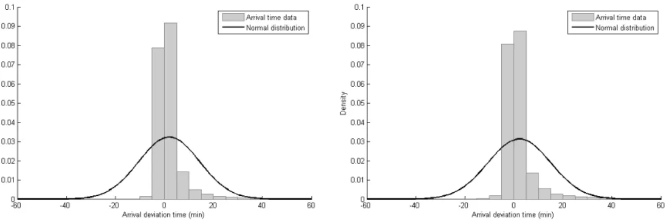
In this paper, one of the issues we want to examine is the distribution of passenger train delays with regard to their size. The basic question is what distribution delays follow and the extent of deviation from the normal distribution. For a passenger the expected delay per train and the probability of a delay of a certain size per train might be relevant for mode and departure choice. In Figure 1 we plot in a histogram the distributions for deviations from planned arrival time for both years in our study. Most frequent are the events that trains are on time, a few minutes early and few minutes late. The distribution is skewed to the right in that there are more delayed trains than early trains. Moreover, there are a number of trains with very large arrival delays (the x-axis is truncated at 60 minutes). We show in Figure 1 also the best fitting normal distribution. As can be seen, the punctual trains are actually more frequent than predicted by the normal distribution, whereas trains with a delay up to 40 minutes are less frequent than predicted by the normal distribution. It is however hard to visually explore in a histogram what happens in the right tail of the distribution.

(13)

Figure 1. Arrival deviation time at the destination in 2008 (left) and 2009 (right)

We therefore proceed to describe the size distribution of delays in terms of percentiles. By basing the analysis on percentiles the relative importance of extreme delays and their share of total delay minutes in the network can be seen. Even if infrequent, their potential impact could necessitate a reallocation of resources from frequent but small-size deviations in order to minimize these extreme events. Table 2 shows what share of the total delay minutes within a given year can be attributed to a certain percentile and the average delay within each percentile. The 10 percent worst delays account for more than 50 percent of total delay minutes for a given year.

Table 2. Percentile share in percentage of total delay minutes in 2008 and 2009

Total no. of observations Average delay (min) Percent of total delay

Percentile 2008 2009 2008 2009 2008 2009 Top 50% 302850 323303 11.56 12.35 91 92 Top 20% 115555 117352 23.25 26.03 70 71 Top 10% 56113 56391 36.94 41.13 54 54 Top 5% 28254 29364 55.07 58.16 41 39 Top 1% 5573 5660 123.54 117.12 18 15

4.1.2 Identification of distribution

Since we ruled out the normal distribution in the previous section, we want to explore what candidate distribution will fit our data better. Distribution fitting can be an alternative due to several reasons: first, the distribution gives a hint on the mechanism behind the causes of delays or to put in the other way around, any mechanism explaining delays should lead to similar

(14)

distributions as the empirical distribution. Related to this is that by means of distribution fitting it can be examined whether delays of different sizes are caused by the same mechanism. Second, distribution fitting allows us to predict probabilities for very low probability events or for delays. Third, examining the distribution helps us find a general pattern that potentially can be applied and compared to regional and international data for delays.

x X x dx

)

e dx

f = Pr ≤ < + =

β

−βx (4)

The complementary cumulative distribution function is thus:

( )

(

)

( )

x x f xdx e X x x F = ≥ = ∞ = −β − Pr

_∫

1 (5)

Whereas we can identify a power-law by a straight line in a double-logarithmic plot, an exponential distribution will exhibit a straight line in a semi-logarithmic plot instead:

(

)

β

− = − dx x F dln1 ( ) (6)

There are related distributions as the power law with exponential cutoff and the stretched exponential. Hence, it is difficult to definitely rule out the power law or to distinguish it from the exponential distribution. The standard way to identify power-law behavior is by spotting a straight line if plotting the logarithm of the inverse cumulative distribution against the logarithm of size (see Figure 2). We pool all observations in order to detect very large delays. As mentioned before, a power law distribution is necessarily bounded by a minimum value and hence applicable only to the tail of the distribution. Additionally, empirical distributions often exhibit signs of boundary effects so that power laws usually only can be confirmed for certain intervals.

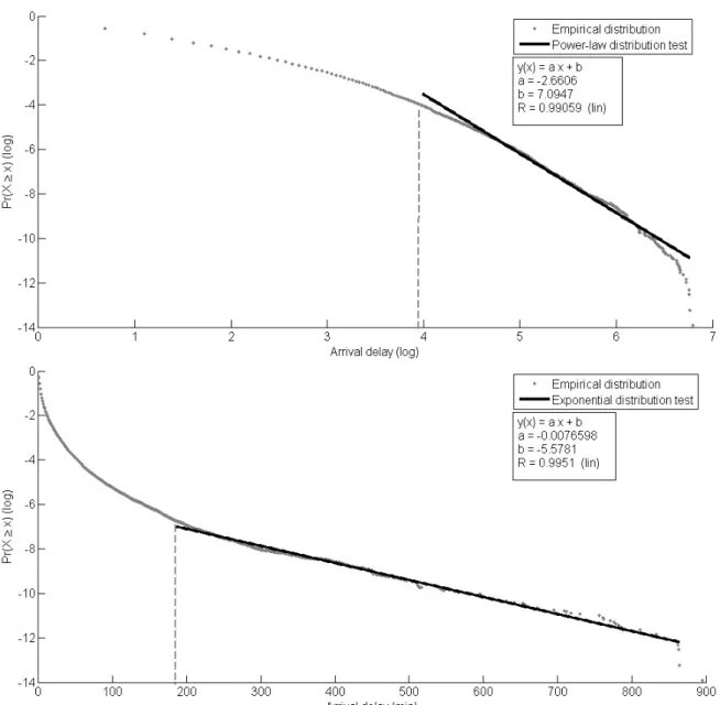
Based on the method outlined in Clauset et al. (2009) and based on maximum-likelihood estimation, different lower boundaries are selected and the power law coefficient is estimated; goodness-of-fit tests are used to select the best fitting lower boundary. Figure 2 shows the result of fitting the data to the power law distribution. It seems that the power law hypothesis cannot be confirmed. For very large delays the power law overestimates the probability for having a delay of that magnitude. However, we cannot rule out that the tail is power law distributed with an exponential cutoff, that is, a combination of both distributions. One reason for this differing behavior for extremely large values is a boundary effect because very large departure delays are registered as cancellation of the train trip instead.

The exponential distribution gives a better fit for the extreme values in the tail (the power law coefficient is 2.6606 and for the exponential distribution the coefficient is .0077). The goodness-of-fit test confirms the visual inspection so that we conclude that the exponential distribution can be used to describe arrival delays of passenger trains in the Swedish rail network.

(16)

Figure 2. Arrival delays with straight line fit of the distribution tail on log-log scale (top) and semi-log scale (bottom)

4.2 Spatial delay distribution

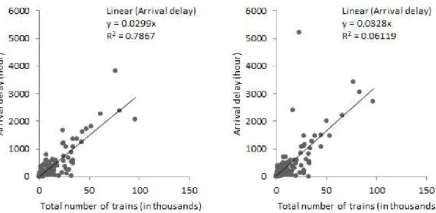
By studying the spatial distribution of train delays it can be distinguished where in the system time deviations are most common, i.e. where the delays occur. The focus is here not on the detailed geographical level, but instead we want to analyze patterns that can be generalized to other cases than the Swedish one. Ex ante we expect to the spatial distribution to be dependent on traffic flows and the connectivity of stations. First, we explore the link between the number of trains arriving at a certain station and the delay minutes recorded at those stations (see Figure 3). There is a strong but a not perfect linear relationship between the number of trains and delay

(17)

size. The strong relationship between trains and delays arises primarily since the probability for delay at a station increases with each train arriving since the per train probability for a delay is constant all things equal. However, a delayed train at one station can affect many other trains arriving in the same station and hence increase delay minutes. This effect will be stronger if the capacity near the station is limited and fully used.

Figure 3. Scatter plot of number of trains versus arrival delay in 2008 (left) and 2009 (right)

Next, similar to the analysis with regard to the size distribution, we analyze the distribution across stations. The difference here is that the stations are a continuous but a discrete variable. Hence, it is more appropriate to examine the rank-size distribution. The ranking is equivalent to the complementary cumulative distribution in the sense that the rank minus one is the frequency for a station having the same or a larger delay size. For the station with most delay minutes the rank is 1 and the frequency is 1 for any other station having the same or more delays. For the station with rank 2 the frequency is 2 of stations having the same or more delays and so on. The cumulative distribution is proportional to the rank-size distribution since the probability of having a station with delays as large as or larger than a certain number is the frequency divided by the number of stations we rank. Figure 4 shows the rank-size distribution of stations with regard to delays aggregated over both years.

(18)

Figure 4. Rank-size distribution of delays at stations for both years on log-log scale (left) and semi-log scale (right)

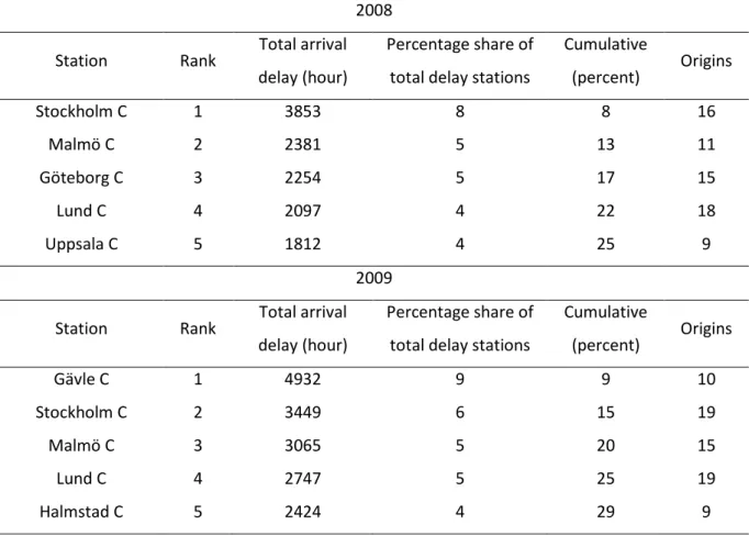
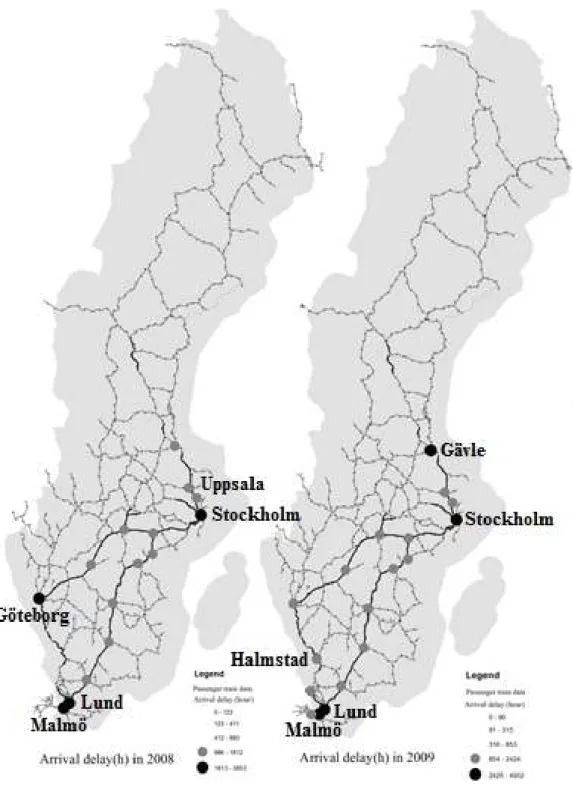
The rank-delay size distribution seems to follow an exponential distribution reasonably well if we compare the log-log and semi-log plots with linear line fit. There are different ways to describe passenger rail networks in topological terms, but besides the number of trains related to every station we can also look at the number of origins that are connected to a certain station. Table 3 shows the five stations with the largest cumulative delay. Compared to the average number of origins, which is 2 origins, the stations with most delays have between 9 and 19 origins. The worst station accounts for between 8-9 percent of all delays and in total the top 5 accounts for 25-29 percent of all delays. Thus, we observe a concentration of delays in certain hotspots, showing the vulnerability of the rail network. In 2009 Gävle is the station with most delay time, whereas it was not in the top 5 in the year before. Gävle is a bottleneck for Swedish trains connecting north Sweden with the rest of the network. Because of harsh winter conditions in the beginning of 2009 many trains in northern Sweden faced problems, since the distances are large and most of the rails are only single track, thus stopping or delaying other trains if a train faces problems. Figure 5 shows the distribution of delays in a map of the rail-network in Sweden.

(19)

Table 3. Rank-Size distribution of delays in 20 stations for both 2008 and 2009 2008 Station Rank Total arrival delay (hour) Percentage share of total delay stations

Cumulative (percent) Origins Stockholm C 1 3853 8 8 16 Malmö C 2 2381 5 13 11 Göteborg C 3 2254 5 17 15 Lund C 4 2097 4 22 18 Uppsala C 5 1812 4 25 9 2009 Station Rank Total arrival delay (hour) Percentage share of total delay stations

Cumulative (percent) Origins Gävle C 1 4932 9 9 10 Stockholm C 2 3449 6 15 19 Malmö C 3 3065 5 20 15 Lund C 4 2747 5 25 19 Halmstad C 5 2424 4 29 9

(20)

(21)

4.3 Temporal delay distribution

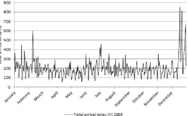
In this section we want to explore the distributions of delays considering daily variations. Figure 6 shows the result of this daily aggregation as a time series for 2009. The most pronounced differences are the large delays in December 2009, a combination of harsh winter conditions and high demand due to the Christmas holiday.

Figure 6. Total delay per day in the Swedish rail network 2009

We sum the delays for every day and use the same procedure described above for delays at stations, that is, we assign the day with most delay minutes the rank 1 and rank the other days accordingly. Figure 7 shows the rank-size distribution of all days in the data set on a log-log scale. Interestingly, the tail of the rank-size distribution seems to follow a power-law. This is a difference in comparison for delay distributions per train (size distribution) and per station (spatial distribution) both apparently following an exponential distribution. Hence, the worst days are very different from a normal day and this might indicate that there is a cascading spread of delays within the network. We can also calculate the probability for an event (certain total amount of delay any given day) to occur in the network. There is a small but positive probability that a daily disturbance double the size that occurred during 2008 and 2009 will occur during a certain future year. The probability is determined by the slope of the linear fit to the tail of the rank size distribution in Figure 7.

(22)

Figure 7: Rank size distribution of days

4.4 Capacity usage and expected delay

In Section 4.2 we saw a strong but imperfect relationship between the amount of delay and the number of trains, that is, more trains means simply more delays. However, as capacity usage increases due to the increased number of trains we would expect that average delay per train increases since congestion would lead to knock-on effects. Capacity usage differs over time and rail demand exhibits periodic cycles within days, weeks and months. In fact, for the years examined here, the number of freight trains reduced by 20% in 2009 compared to 2008 due to the economic contraction. In a sense, these aforementioned variations allow us to examine the link between capacity usage and the expected delay per train. All things equal, we would expect that the average delay increases as capacity usage increases.

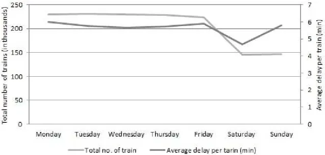
First, we examine the within week variation (see Figure 8). The total number of passenger trains is constant across weekdays at circa 230 thousands whereas during weekends the number falls just below 150 thousands, which corresponds to a decreased capacity usage of about 35 percent during weekends. Hence, we would expect a significant dip in average delays since capacity is freed up during weekends. Whereas there is a considerable dip during Saturdays (19%) no such effect can be observed for Sundays.

In Figure 9 we aggregate the data for months and compare total number of trains and average delay per train per month. Again, no clear-cut relationship between the number of trains and average delay emerges. The correlation coefficient is -0.26, implying there is a tendency that the per train delay is decreasing as capacity usage is increasing.

(23)

Figure 8: Total number of trains and average delay per weekday

Figure 9: Arrival delay and total no. of trains aggregated over months

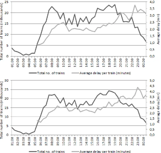
It could be argued that the weak (and actually negative) link between capacity usage and average delay is due to the fact that the traffic is decreasing in off-peak times whereas it is the same during peak-times and hence that the missing link is just an illusion. In order to investigate this issue we identify peak-times by plotting the total number of trains using the rail network at any given hour and the average delay per train (see Figure 10). We can identify two peak-periods: one during morning 7-8am and one during afternoon/early evening 4-7pm. Moreover, we can see that there is only a weak, if any, relationship between peak-demand and average delay. The average delay increases in the late evening hours when the number of passenger trains is

(24)

decreasing. Because of the low number of trains during the night it is not meaningful to compute an average delay and we exclude those hours in Figure 10. The correlation coefficient is -0.56 for 2008 (-0.52 in 2009); if we exclude the night hours which bias the average delay upward the correlation coefficient is -0.03 for 2008 (-0.12 in 2009). Hence, the link between capacity usage and expected delay per train is best described as weak, although extreme delays might bias upward the average delay estimates.

Figure 10. Number of trains versus average delay per train in 2008 (top) and 2009 (bottom)

(25)

5. Implications

i) Societal costs of delay: Even though there is a difference between delayed trains and delayed passengers, since passenger volumes can differ from train to train, the distribution of train delays can give an idea about passengers’ variation in travel time. So, an obvious consequence when identifying delayed trains is that it is necessary to weight the train delays with the number of affected passengers. Thus, by analyzing delay distributions it may, to some extent, be possible to predict delays in the network as well as draw conclusions about how this impacts passengers’ travel time variability.

To be able to weight the delayed trains with the number of delayed travelers and to be able to state something about the travelers’ valuation of these delays, one has to make some assumptions. First we assume the average number of seats per train to be approximately 200, whereas the load factor for the Swedish trains, i.e. the percentage of seats filled, is 54 percent in both 2008 and 2009 (SJ, 2010). With more than 700,000 trains running the national rail network during 2008 and an average delay per train of 5.4 minutes, the total delay for all trains are more than 64,000 hours, revealing that the total delay for all passengers are almost 7 million hours. By using a division made by Banverket (Lundin, 2007) we can assume that 48.7 percent of these are private regional trips, 37.7 percent are private national trips and 13.6 percent are business trips. The Swedish Transport Administration has in their ASEK 5 report (Trafikverket, 2012) established time values which form the basis of socioeconomic calculations, where the time value indicates how much a traveler is willing to pay to reduce travel time. The recommended time values for long-term private regional trains are 71 SEK/hour, for private national trains 98 SEK/hour and for business trips 331 SEK/hour in 2010 monetary value. Moreover, delays in public transport are valued with regard to average delay time, i.e. the average deviation from the scheduled travel time. ASEK 5 recommends that this deviation, i.e. the delays, should be valued 3.5 times the time value. The calculated delay cost for private regional trips is therefore 839 million SEK, for private national trips 896 million SEK and for business trips 1092 million SEK. In total, the societal costs for the delays analyzed in this paper are 2,827 million SEK. With a linear valuation of delay time, this implies that the 10% worst delays cost the society more than 1.4 billion SEK. With a non-linear, increasing valuation the share of total societal costs for the very large delays would be larger than their share in total delay minutes, that is, more than 54%.

ii) Reliability vs vulnerability: Travel time is one of the largest costs associated with transportation; hence, reduction of travel time is very important and therefore justifies improvements in transportation infrastructure. Naturally, how travel time is valued is a central issue when planning transportation projects. The analysis in the preceding section shows

(26)

however, that focusing on mean travel times and describing variability by standard deviation is misleading. Considering the thick tails of the delay distribution it raises the question whether all travel time variations have the same value, regardless of size and frequency. With a linear valuation of time approach, the value increases proportionally with delays, even when there are very large delays. However, up to now there has been limited research on the valuation of very extreme delays. Hence, there is no clear relation between train delays and value of time that could be used in a satisfactory way over the whole distribution. If we instead consider a non-linear valuation of time, long delays might have a higher value or lower value compared to short delays. Since we have skewed distributions, and not normal distributions as earlier has been assumed, this has implications for how to measure the VTTV. In usual stated preference as well as revealed preference studies, where train delays have been assumed to be normally distributed, the VTTV has been based on standard deviations. Our results show that the traditional means of valuing reliability through standard deviation or average delay is a poor measure of variability. Instead the results suggest a better valuation measure should consider the whole delay distribution, for example by valuation of percentiles. We have found that the worst 10% of all delays account for more than 50% of all delay minutes in Sweden, that is, circa 1.4 billion SEK. Thus, vulnerability cannot be disregarded.

iii) Targeting weak-spots: As outlined in the previous section we do not know exactly the societal costs associated with the thick tails of the delay distribution. However, the analysis in this study reveals that the few extreme and large delays cannot be neglected, an important implication when prioritizing between reliability improvements. Moreover, our results indicate that measures aiming at decreases in average delay would not have a major impact on rail network reliability, or in other words, strategies aiming to improve reliability equally over the system would not be efficient. Instead measures targeting the identified vulnerabilities in size, space and time are expected to be more efficient in reducing travel time variations. One can argue that large delays occur where capacity is used the most, because there are many links, nodes and trains that can be affected and once affected influence other links, nodes and trains. In other words, the extremely unevenly capacity usage that is characteristic to rail networks (and other complex networks) is in itself a cause for large delays. Once we account for the number of trains the average delay per train (and per train kilometer) is not significantly affected. Hence, large delays are a sign that we have large transportation demand and there will be no easy way to prevent delays. There are nevertheless some possible policy measures that can be used to target the problem. The reason is the revealed extremely uneven distribution of transport demand and delays over time and space. These distributions suggest that investment in capacity, reinvestments and ordinary maintenance

(27)

measures should be spread not uniformly across the rail network but be focused on problematic hotspots. Even now investments and maintenance are not carried out evenly but capacity investments and reinvestments should probably be more extremely distributed. Measures undertaken for improving reliability outside the central nodes are with a high probability without any major effect on overall performance of the rail network since they are of minor importance of the functioning of the whole network. For this reason, our results provide some (even if limited) insights on the impact of measures on performance outcomes and are therefore of some value for cost-benefit analysis of measures targeted at improving reliability and increasing capacity.

iv) Endogenous vs exogenous causes: We find that individual train delays have exponentially distributed tails and that the delays over days have power-law distributed tails. This difference might be caused by cascading effects as a disturbance is propagated through the system. Hence, even if we think and can see in the data that exogenous factors like weather conditions matter for the probability and severance of breakdowns, the causes are to some extent still endogenous to the rail network and most probably there is some interdependence and combinations between various endogenous and exogenous causes. Endogenous in this context means that the rail network has a complex structure that is prone to be robust with respect to disturbances at most times and places but that at some times and places the network is fragile to disturbances, propagating initial small and geographically limited disturbances through connecting links, nodes and the rolling stock itself to larger and more widespread breakdowns in the transport network.

v) Predictable vs unpredictable delays: We have to acknowledge that many delays are unpredictable. Our data analysis reveals that the delays that matter most have extremely low probability. However, we can in predict something, namely, the probability for an event of a given seize. For example, we can predict that a major breakdown will occur at least one time next year, however, we still do not know where and when. If we could predict where and when, they would not occur. However, based on our analysis of delay distributions at stations we can say that measures undertaken to reduce the importance of central nodes as stated above (regardless whether it is a steering computer or a marshaling yard) would milder the consequences of disturbances. Also keeping a network of express-busses as backup could be a way to milder the consequences of the very large delays.

(28)

6. Conclusions

To the best of our knowledge this is the first study in its kind related to passenger transportation on rail. The analysis of delay distribution facilitates the selection of appropriate methods for valuation of rail reliability and thus for cost-benefit analysis of rail investments and other measurements. More specific, our analysis suggests that standard deviation is not an appropriate measure of reliability risk. It seems that very few extremely large delays matter for the total amount of delay and not the many small delays. However, only a sound valuation method can answer the question whether society would benefit from reducing the number of delays in general or from preventing the extremely large delays.

In order to know whether it is more important to target the many small or the few very large delays, we suggest more research on how many passengers are affected and how they value different delay sizes. Up to now, there is no research about neither societal nor individual willingness to pay for avoiding extreme delays. Moreover, we would expect that the network structure causes many extreme delays so that an analysis of network topology might be a fruitful avenue of research. A better network organization, for example by decentralizing steering, backup capacity, extreme focus on hubs with regard to maintenance and coupling the express bus network to the train network, might reduce the vulnerability of the rail network.

Acknowledgements

We would like to thank Inge Vierth, Swedish National Road and Transport Research Institute, for useful comments and suggestions and Roger Pydokke for generously sharing data.

References

Banverket, 2010a. Banverkets årsredovisning 2009 .

Banverket, 2010b. Järnvägssektorns utveckling. Banverkets sektorsrapport 2009.

Bates, J., Polak, J., Jones, P., Cook, A., 2001. The valuation of reliability for personal travel. Transportation Research Part E: Logistics and Transportation Review 37(2-3), 191-229.

Berdica, K, 2002. An introduction to road vulnerability: what has been done, is done and should be done. Transport Policy 9(2), 117-127.

Börjesson, M., Eliasson, J., 2011. On the use of “average delay” as a measure of train reliability. Transportation Research Part A: Policy and Practice 45(3), 171-184.

(29)

Briggs, K., Beck, C., 2007. Modelling train delays with q-exponential functions. Physica A: Statistical Mechanics and its Applications 378(2), 498-504.

Brons, M., Rietveld, P., 2011. Beyond Punctuality: Appropriate Measures for Unreliability in Rail Passenger Transport. In van Nunen, J.A., Huijbregts, P., Rietveld, P. (eds.) Transitions Towards Sustainable Mobility: New Solutions and Approaches for Sustainable Transport Systems. Springer. 175-192

Bruinsma, F., Rietveld, P., Vuuren, D.V., 1999. Unreliability in Public Transport Chains. World Transport Research - Selected Proceedings of the 8th World Conference on Transport Research 1, 59-72. Cambridge Systematics Inc, 1998. Multimodal Corridor and Capacity Analysis Manual. NCHRP

Report 399. Transportation Research Board. Washington D.C.

Carrion, C., Levinson, D., 2012. Value of travel time reliability: A review of current evidence. Transportation Research Part A: Policy and Practice 46(4), 720-741.

Clauset, A., Rohilla Shalizi, C., Newman, M.E.J., 2009. Power-law distributions in empirical data. SIAM Rev 51(4), 661-703.

Department for Transport, 2009. The Reliability Sub-Objective, TAG Unit 3.5.7. United Kingdom: Department for Transport.

Elefteriadou, L., Cui, X., 2007. Travel Time Reliability and Truck Level of Service on the Strategic Intermodal System. University of Florida. Transportation Research Center. Gainesville.

Eurostat, 2011. Passenger Transport Statistics. European Commision. Last updated: 28

November 2011. Accessed: 7 September 2012.

<http://epp.eurostat.ec.europa.eu/statistics_explained/index.php/Passenger_transport_stati stics#Rail_passengers>

Fosgerau, M., Hjorth, K., Brems, C., Fukuda, D., 2008. Travel time variability: Definition and valuation. 2008:1, Denmark: DTU Transport.

Ghoshy, S., Banerjee, A., Sharma, N., Agarwal, S., Gangulyz, N., Bhattacharya, S., Mukherjee, A., 2011. Statistical analysis of the Indian railway network: a complex network approach. Acta Physica Polonica B Proceedings Supplement No 2. Vol. 4

Goverde, R., Hooghiemstra, G., Lopuhaä, H., 2001. Statistical Analysis of Train Traffic, Delf, The Netherlands: DUP Science.

Goverde, R., 2005. Punctuality of Railway Operations and Timetable Stability Analysis, s.l.: TRAIL Research School for Transport, Infrastructure and Logistics, Delft University of Technology.

Government Offices of Sweden, 2011. ”Railway”. Last updated: 25 October 2011. Accessed: 7 September 2012. <http://www.regeringen.se/sb/d/11655/a/60129>

(30)

Güttler, S., 2006. Statistical modelling of Railway Data, s.l.:M.Sc. thesis, Georg-August-Universität zu Göttingen Higgins, A. & Kozan, E., 1998. Modeling train delays in urban networks. Transportation Science, 32(4), 346-357.

Herrmann, T.M., 2006. Stability of timetables and train routings through station regions. Swiss Federal Institute of Technology.

Lindgren, J., Jonsson, D.K., Carlsson-Kanyama, A., 2009. Climate adaptation of railways: lessons from Sweden. European Journal of Transport and Infrastructure Research (EJTIR) 9(2), 164-181. Lundin, M., 2007. Samhällsekonomiska kostnader för störningar i järnvägsnätet. Rapport 2007:6.

Transportforskningsgruppen Borlänge.

Nilsson, J.E., 2002. Restructing Sweden’s railways: The unintentional deregulation. Swedish Economic Policy Review 9, 229-254

OECD, 2010. Improving reliability on surface transport networks. Transport Research Centre: International Transport Forum.

Paulley, N., Balcombe, R., Mackett, R., Titheridge, H., Preston, J., Wardman, M., Shires, J., White, P., 2006. The demand for public transport: The effects of fares, quality of service, income and car ownership. Transport Policy 13(4), 295-306.

Peer, S., Koopmans, C.C., Verhoef, E.T., 2012. Prediction of travel time variability for cost-benefit analysis. Transportation Research Part A: Policy and Practice 46(1), 79-90.

Rietveld, P., Bruinsma, F.R., van Vuuren, D.J., 2001. Coping with unreliability in public transport chains: A case study for Netherlands. Transportation Research Part A: Policy and Practice 35(6), 539-559.

Schwanhäußer, W., 1974. Die Bemessung der Pufferzeiten im Fahrplangefüge der Eisenbahn, Veröffentlichungen des Verkehrswissenschaftlichen Institutes der Rheinischen-Westfälischen Technischen Hochschule Aachen, Heft 20, Aachen

Trafikanalys, 2012. Järnvägstransporter 2012, kvartal 1. Statistik 2012:10. Published 13 June 2012. Trafikverket.

Trafikverket, 2012. Samhällsekonomiska principer och kalkylvärden för transportsektorn: ASEK 5. Version: 2012-05-16.

Transek, 2006. Restidsosäkerhet och förseningar i vägtrafik - Effektsamband för samhällsekonomiska beräkningar. 2006:1.

van Loon, R., Rietveld, P., Brons, M., 2011. Travel-time reliability impacts on railway passenger demand: a revealed preference analysis. Journal of Transport Geography 19(4), 917-925.

Yuan, J., Goverde, R., Hansen, I.A., 2002. Propagation of train delays in stations, Southampton: Computers in Railways VIII, WIT Press.

(31)

Yuan, J., 2006. Stochastic Modelling of Train Delays and Delay Propagation in Stations, Delft: Delft University.