125 1988
Estimation of the effects of
counter-measures on different types of accidents in the presence of regression effects
Stig Danielsson
Reprint from Accident Analysis & Prevention, Vol 20, No 4, pp. 289-298, 1958
vVäg06/1 Efi/( Statens vag- och trafikinstitut (VTI) e 581 01 Linkoping 8t,tlltet Swedish Road and Traffic Research Institute * S$-581 01 Linkoping Sweden
Printed in Great Britain. © 1988 Pergamon Press plc
ESTIMATION OF THE EFFECTS OF
COUNTERMEASURES ON DIFFERENT TYPES
OF ACCIDENTS IN THE PRESENCE OF
REGRESSION EFFECTS
STIG DANIELSSON
Swedish Road and Traffic Research Institute (VTI), S-581 01 Linköping, Sweden (Received 23 August 1985; in revised form 5 June 1987)
Abstract In an earlier paper [Danielsson, 1986] , we studied the problem of estimating the safety effect of a countermeasure on the expected number of accidents at road junctions when
high-accident sites are selected for the study. Often, however, the countermeasure leads to varying effectiveness on different types of accidents. This paper is a generalization in that we estimate
effects of countermeasures for each type of accident. A major result, for which empirical support
is provided, is that the expected regression effect is the same for all types of accidents.
1. INTRODUCTION
In an earlier paper [Danielsson, 1986], we described the problem of the regression effect which can occur in before-and-after studies [for detailed descriptions see Briide and
Larsson, 1982; Hauer, 1980a, 1980b; Hauer, 1986; and Hauer and Persaud, 1983]. In
the paper, we proposed a method of purely estimating the effects of countermeasures despite the presence of regression effects.
Unfortunately, there are in practice further complications with the regression effects.
Assume, for example, that we wish to study the number of accidents at road junctions to determine whether a particular countermeasure has any (positive) effect. Naturally, the effectiveness of the countermeasure most often varies between different types of accident. The total effect (on all types of accidents) can then be interpreted as the average effect. One possible way to estimate this effect is obtained if junctions are selected at
random and an estimate then made of the total (constant) effect. In many cases, however,
only those junctions which are especially prone to accidents are selected, so that it is hardly possible to expect that the accident composition at the selected junctions is normal. An estimate of the total effect from such a sample may therefore be extremely misleading.
One way of avoiding this complication is to estimate the effect for each type of accident. If this can be done, it is then possible to estimate the total effect for any accident composition at the junctions.
2. FORMULATION OF THE PROBLEM
Consider a junction which under normal conditions has mean values ml, m2, . . . ,
mp per time period for p mutually exclusive types of accident. Examples of such types are (for cars) single-vehicle accidents, rear-end collisions, overtaking accidents, etc. When introducing a countermeasure, we assume that the expected numbers of accidents are changed to
041ml, azmz, . . . ,apmp. The total expected number of accidents
m=m1+m2+...+mp
290 S. DANIELSSON
is then changed to am, where
alml + azmz + . . . + (1me
_ m .
We call (1 a) the total safety effect of the countermeasure, while (1 al), . . . , (1 ap) are the effects on the different types of accidents.
If a junction is selected at random from a population of similar junctions, a correct estimate of a can be obtained by studying the effect of the countermeasure on the total number of accidents. The estimate of (1 - a) can then be regarded as the estimated effect of the countermeasure for an average junction. This is obviously not true if the junction is not selected at random. In such a case, it would be necessary to try to estimate
the individual effects 1 dl, 1 az, . . . , 1 (xp, and then to use these to estimate
the total effect 1 - a for a given junction.
Consider a period before the implementation of a countermeasure and let
X., = the number of accidents of type j occurring at the junction studied,
j=1,2,...,p.
We make the assumption that different X,- are independent and Poisson distributed with
parameters m1, m2, . . . , mp respectively. We also define the total number of accidents
X.],
'M
e
X=
N ll bd
which is, of course, Poisson distributed with the parameter
We further assume that the junction has been selected for study because the total number of accidents is large, i.e. that
X 2 k.
The conditional distribution for the total number of accidents at a selected junction
is thus what can be termed truncated Poisson [see Danielsson, 1986; Hauer, 1980b; and
Hauer and Persaud, 1983] according to
,
_
_
>
_ pr(m),
_
p,(m)
P(X r|X_k) qk(m), r k,k+ 1,...
(1)
where
mm = en? [; qk<m> = gkpxm).
(2)
Now we are interested not only in the (conditional) distribution for X but mainly in the
distribution for (Xl, X2, . . . , Xp) given that X 2 k.
The simultaneous distribution
becomes
r
-,m
,m
p1(m1) p2( 2) pp( P); all rj : 0,1, 2, . . . , p'(r1, . . . , rp) =
WU )
r1+r2+...+rp2k. (4)
3. ESTIMATION OF EXPECTED REGRESSION EFFECTS AND COUNTERMEASURE EFFECTS FOR DIFFERENT TYPES OF ACCIDENT
Before studying the estimation procedures in detail, it can be instructive to consider
a practical example.
[
3.1 A practical example illuminating the regression effects
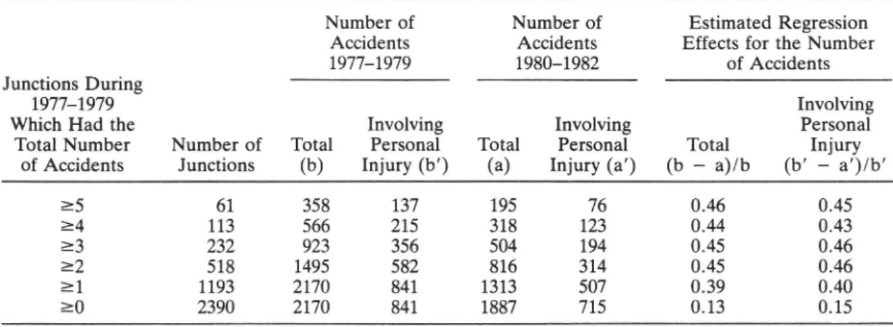
In the example in Table 1, we consider rural junctions in Sweden which have been unaltered during the period 1977 1982. We study the total number of accidents but also the accidents involving personal injury. The years 1977 1979 are regarded as the before period, and the selection criterion (X 2 k) is based on the total number of accidents. The years 1980 1982 are regarded as the after period, and by comparing the before and
after accidents we have estimates of the regression effects, since no countermeasure has
been implemented at the junctions during 1977 1982.
The estimated regression effects in Table 1 are fairly high for different selection criteria. We can also notice that the total accident number is lower in the after period than in the before period. This is probably due to a general trend in the accident development. Therefore, the true regression effects are lower than those calculated in
the table, but we have not made any corrections.
The results in Table 1 can be formulated in the following hypothesis: the regression effects are the same for all types of accidents as for the total number of accidents. Since an example is not a proof, this hypothesis is proved in the next section.
3.2 Expected regression effects for different types of accidents
In Danielsson [1986], we showed that the expected regression effect for the total number of accidents is
R = uk(m) _ m : Pk 1(m) MU") Che 10"), where
MO") = EIXIXZ kl-
(5)
Table 1. Estimated regression effects for the total number of accidents and accidents involving personal injury at rural junctions in Sweden
Number of Number of Estimated Regression
Accidents Accidents Effects for the Number
1977 1979 1980 1982 of Accidents
Junctions During
1977 1979 Involving
Which Had the Involving Involving Personal
Total Number Number of Total Personal Total Personal Total Injury of Accidents Junctions (b) Injury (b') (a) Injury (a') (b a)/b (b a )/b
25 61 358 137 195 76 0.46 0.45 24 113 566 215 318 123 0.44 0.43 23 232 923 356 504 194 0.45 0.46 22 518 1495 582 816 314 0.45 0.46 21 1193 2170 841 1313 507 0.39 0.40 20 2390 2170 841 1887 715 0.13 0.15 ..
292 S. DANIELSSON
We now want to determine the regression effect for accident type j, i.e.
: ka(mj) _
m,-Ri Mk(mj)
where
nk(m,-) = ElelX > k]-
(6)
Conditional to X = r it holds that X]- is binomial distributed with expected value
r {mi/m. Therefore,
ElleX z k] = & p;(m)E[X,-|X z k, X = r]
Mk(mj) : r=k 0° , oo , mi
= 2 pr(m)E[X,-|X = r] = 2 Mm) ' r;
r=k r=k : ElE[X|X > k] : T_j . m qk 1(m) = m_ qk 1(m). (7) m m qk(m) ] qk(m)By substituting (7) into (6) we get
Rj=1 M M R. (8)
(Ik 10") _ Che 10") _
This means that the expected regression effect is the same for all types of accidents. The result may appear slightly surprising, but with a little afterthought it is natural and even intuitive. The extra accidents generated by the condition X 2 k obviously have to be distributed proportionally to ml, m2, . . . , mp for the different types of accidents. 3.3 Estimation of the expected accident numbers for a single junction
In order to estimate the different m,- for a single junction, we construct the likelihood
function for x1, x2, . . . , xp (which are the observed number of accidents of different types)
of: p'(x1, . . . ,xp)
We then seek the m,- which maximize [see (4)]
I = In (of) = 2111 (px,-(mi)) = In (qk(m))
ålen m,-
åln (xi!)
ln (Z %).
(9)
r=k By differentiating (9) we obtain<9_ = & _ ___r=k
(r _ 1)! = & _ _qk 1(m)
(10)
drnj Inf åå __: inf qk(n1) r=k r!If the derivatives in (10) are set equal to O we obtain
(lk 10") .
- = - ' = 1 2 . . . , . 11
The right-hand term in (11) is, of course, the earlier calculated E [X,-IX 2 k], i.e. the
maximum likelihood (ML) estimates above are identical to the moment estimates. We have shown earlier [Danielsson, 1986] that the ML estimate for m can be calculated from the equation
x=m-%j§T )),
(12)
and this result is, of course, also obtained if the equations in (11) are summed. From (11) and (12) we can state that
_ Hie 10") _ x
x.] m] qk(m) m- ' ,] m (13) i.e. if mf, j = 1, 2, . . . , p, and m* are the ML estimates, we obtain the following
simple relations
x.
mik : m* ' ;] (14)
To obtain the ML estimate of all mi, we therefore need only solve one equation nu-merically [the ML equation for m in (12)]. The simple relations in (14) then give the required estimates.
Since according to (8) the regression effects are the same for all types of accidents, it is sufficient to estimate R according to
R* = _. (15)
Finally, we can also determine an intuitive estimate of m,- by analogy with Hauer s estimate of m [Hauer, 1980a, 1980b]. Hauer has proposed the following estimate of m
._ o ifx=k
m_{x ifx>k.
(16)
In agreement with (16) we estimate m,- with
. _ o ifx=k
'" {x}- ifx>k.
(17)
The estimator m, is unbiased since [see (7)]
. _ _ , _ m- __ Che 10") _ Älv/((m) E[mj] _ M0711) Pk(m)k ;; _ m,- < qk(m) m qk(m)> = (Ch 10") _ Pk 1(m)) : m-] %(m) ], where kPk(m) = mPk 1(m)- (18)
3.4 Simultaneous estimates of regression and countermeasure effects
Assume that at n junctions we wish to introduce a countermeasure which for different types of accidents has the constant effects 1 al, 1 az, . . . , 1 ap, respectively. MP 20 d'.-D
294 _ S. DANIELSSON
Regardless of the nature of the site, we assume that the effects are fixed. Of course, in many practical situations this is unrealistic because remedial measures interact with their environment. We apply the following notation for junction no. i:
Xji
y..]1 the number of accidents of type j before the countermeasure is implemented;the corresponding number of accidents after the countermeasure is imple-mented (during an equal duration of time);
P
X.,- = 2 X,»,- = the total number of accidents in the before period;
j=1
Y,- :
"M"
*»
Yi,- = the total number of accidents in the after period.
'ä
- || ...a
In Section 2, we studied the distributions for variables of the type Xi,- (X.,- is assumed
to be truncated in ki). We assume that Yi,- is Poisson distributed with expected values
(lj ' mji Where
m,,- = the expected number of accidents of type j before implementation at the junction studied.
Furthermore, it holds (with assumed independence between the Y ) that Y.,- is
Poisson distributed with expected values a.,- - m.,- where
"M
s
£5
m., = the expected total number of accidents before implementation
J=1 at the junction,
p mi
a.,- = z ;??! a, = the total effect of the countermeasure at junction no. i.
j=1 -i
Now, the problem is to estimate the countermeasure parameters al, . . . , up and or,- by using directly all the data x],- and y],- from all junctions. In the appendix the following maximum likelihood estimates (ML estimates) of a,- and m],- are derived
Z yii aj=i,;= l ;j=1,2,...,p (19) 2 mil" i=1 . qki_1(m.,-) + _ + _ j: 1, 2, . . . ,p 20
' qk.(m..)
m " _ x
i= 1. 2. . . . .n.
( )
This complicated equation system can be solved by a rather simple numerical method, which is outlined in the appendix.
We observe that the estimator of a,- in (19) is of the same type of quotient as in the case where a common effect for all accidents is estimated [see Danielsson, 1986]. The argument in Danielsson [1986] for judging the uncertainty of af will be fully equivalent also here. We will therefore not concern ourselves with these details.
Finally, we note that it is also possible to estimate a,- by using the intuitive estimates of mi,-. The reasonable estimate of a,- is of course
n 2 Y _ i=1 j_ n 2 mji i=1
,
(21)
where
A 0 if x.,- = k, m'i = .
] xi; 1fx.,- > ki'
5. COMMENTS ABOUT THE PRACTICAL APPLICABILITY OF THE ESTIMATION METHODS
In the preceding section we have derived the ML estimators of the different or,-. The estimators are rather complicated to handle and there is a need for simpler and quicker estimation methods even though they are less efficient. We begin the discussion with the ML estimators and then successively introduce some simplifications.
(i) ML estimators. The estimator of a,- derived from (19) and (20) is rather com-plicated, even if the multidimensional problem can be reduced to a sequence of one-dimensional problems as described in the appendix.
The form of the ML estimator (19) is simple provided the estimators of m are determined. Thus, simplified estimators can be obtained by replacing the denominator in (19) with estimators of m other than the ML estimators.
(ii) ML-like estimators. In (21) we have proposed a simple estimator of a,- which
does not require any complex calculation. The estimator of (x,- can be formulated
&,- = the total number of type j accidents in the after period divided by the corre-sponding total number in the before period for the sites which fulfill the selection criteria plus one type j accident.
Another estimator can be derived from (14). Using only the before data for esti-mating m , the ML estimator is
m? - = mi? ji, (22)
where mf'; easily can be calculated from [see (12)] qk- 1(m-i)
-i _ -i "" ", "'_- 23
qk,-(m-i) ( )
Then, the estimator of oc,- is
21 in
af = I-
.
(24)
(iii) Estimators by explicit use of the regression effect. If the regression effect R,- in (5) for the total number of accidents at each site is known, then or, can be estimated
from
2 in
a- = ,, l=1
.
(25)
Z (1 _ Ri)xji i=1
The result follows from the definitions (5) and (6) and from the fact that all accident types have the same regression effect [see (8)].
296 S. DANIELSSON
In practice, the different R,- very seldom are known. However, in some cases it is possible to assess the regression effect and the estimate in (25) can be determined with this estimate of R,. One way to estimate R,- is to use the Strike method proposed by Briide and Larsson [1982]. Formula (25) is especially simple when all sites have the same regression effect R. Then we have
Z in
(ij = 1:1 n . (26)
(1 _ R) 2 xii
i=1
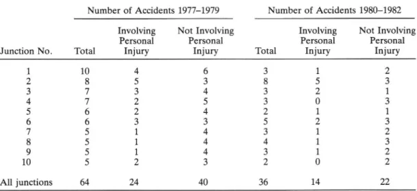
(iv) An illustrative example. From the material in Table 1 , 10 junctions are selected, all with total accident numbers of at least 5 in the before period. The selected junctions are presented in Table 2a.
Let 1 dl, 1 az, and 1 a be the countermeasure effects for accidents involving
personal injury, accidents not involving personal injury, and all the accidents respectively. It is interesting to compare the estimates &], af and 62,- proposed in (21), (24), and (26). It is worth noting that there is no real countermeasure effect, but instead we seek to estimate a general downward effect in the whole population of about 15%.
It is very easy to compute the estimates proposed in (21). Consider e.g. the accidents involving personal injury. Then
To compute aik in (24) it is necessary to solve the equation
q4(m-"i) 10 = m.* _ 1 (150773)
for junction No. 1, and then the corresponding equations for the other junctions. The definition of qk can be found in (2). The solution of the equation above is
m. ; = 9.8, and then
4
mfl = 9.8 ' E = 3.92.
Table 2a. Number of accidents for selected junctions divided with respect to personal injury Number of Accidents 1977 1979 Number of Accidents 1980 1982
Involving Not Involving Involving Not Involving
Personal Personal Personal Personal
Junction No. Total Injury Injury Total Injury Injury
1 10 4 6 3 1 2 2 8 5 3 8 5 3 3 7 3 4 3 2 1 4 7 2 5 3 O 3 5 6 2 4 2 1 1 6 6 3 3 5 2 3 7 5 1 4 3 1 2 8 5 1 4 4 1 3 9 5 1 4 3 1 2 10 5 2 3 2 0 2 N A A O U) ON _ A N N All junctions 64
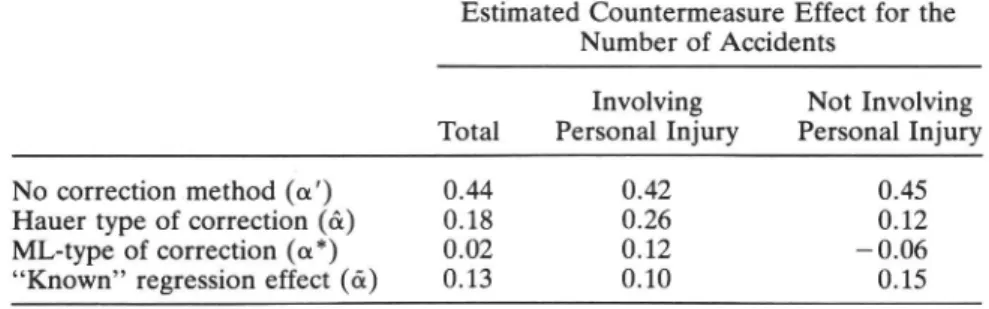
Table 2b. Countermeasure effects estimated with different methods Estimated Countermeasure Effect for the
Number of Accidents
Involving Not Involving Total Personal Injury Personal Injury
No correction method (a') 0.44 0.42 0.45
Hauer type of correction (&) 0.18 0.26 0.12
ML-type of correction (a*) 0.02 0.12 0.06
Known regression effect (a) 0.13 0.10 0.15
For the observations 8, 7, 6, and 5 the corresponding m.*-values are 7.4, 6.0, 3.8,
and 0. Then it is easy to compute all mi", and we have E mf,- = 16.0. Therefore
14
* = _ = 0.1 16_0 0.88.
From Table 1, we can conclude that the regression effect is about 35% (since there is general downward secular trend of about 15%). Therefore we have from (26) (assuming the same regression effect at all sites)
14
1= m =
0-90-&
Without any compensation of the regression effect, the estimate of al is
_3
"24
I
011 = 0.58.
The results of all computations are presented in Table 2b. It is obvious that the countermeasure effects (in this case, the secular changes) are seriously overestimated if no correction method is applied. The various correction methods give similar results,
but the estimates are rather unstable. An exception is the estimate &, which, since it
utilizes the known regression effect, is quite reasonable.
REFERENCES
Briide U. and Larsson J., The regression-to-mean effect. Some empirical examples concerning accidents at road junctions. VTI Report 240, 1982.
Danielsson S., A comparison of two methods for estimating the effect of a countermeasure in the presence
of regression effects. Accid. Anal. Prev. 18, 13 23, 1986.
Hauer E., Bias by selection: Overestimation of the effectiveness of safety countermeasures caused by the process of selection for treatment. Accid. Anal. Prev. 12, 113 117, 1980a.
Hauer E., Selection for treatment as a source of bias in before-and-after studies. Traffic Eng. Control 8/9, 419 421, 1980b.
Hauer E., On the estimation of the expected number of accidents. Accid. Anal. Prev. 18, 1 12, 1986.
Hauer E. and Persaud B . , Common bias in before-and-after accident comparisons and its elimination. Transpn.
Res. Rec. 905, 164 174, 1983.
APPENDIX
Maximum likelihood estimates of a,- and m],- in Section 3.4
We wish to estimate the countermeasure parameters al, . . . , or,, and a.,- by directly using data from all n junctions. The total likelihood for the observed values x,,- and y,,- ( j = 1, 2, . . . , p, i = 1, 2, . . . , n) wrll
298 S. DANIELSSON
be [see (2) and (4)]
of: HPK-Mi, x2ia ' ' ' a xpi) ' py1i(a1mli) ' ' ' ' ' Pym-(07mm) i=1
ln (f) = i {21n(p.,.(m,-.-)) ln (cz/(xml)) + & ln (pm-mp»)
i=1 j=1 j=1(m i) )
r!
P P P
" E (limit + 2 Y ln (aj ' mii) "' Z
1110010}-i=1 f=1 N " co n p P 2 {Z x,,- ln m,,- z ln (xp-!) ln ( i=1 j=1 j=1 r k ,-=1 (A1)
Differentiating (Al) gives
al " y,,
_ = _ ml + _a = 19 29 3
do, I; 1 221 &] ] p
(A2)
al =x11 qkl 1(m )a,-+ y , ._12] 19 2, ' 7 P
Öm . mi; qki(m.,-) mji l _ 7 7 ' a "'
If the derivatives in (A2) are set equal to 0 we obtain
Z Y
aj='T=1 ;j=1,2,...,p, (A3)
2 mfi
i=1
man, ,-=1,2,_._,p
qki(m_i)
f
f'
1,2, . . . ,n.
(A,,
Summing (A4) with regard to j, we obtain _,- 61__k_1(m.,-) P
-i =x.,-.+y, ; i=1,2,...,n. A5
61k,-(mi) +120ij ( )
Since from definition
P
z ajmji = CL,- ° m.,', (A6)
j=l
where a.,- is the total effect for junction no. i, for each given a.,- it is now easy to solve m.,- from (A5) by using the method proposed by Danielsson [1986]. If we know a,- we can then solve m,,- from
mi; = m.,' ' x]! + y ; I = 1, 2, . . . , , (A7)
x.,- + y., a.,-m.,- +
cc,-m.,-which are obtained from (A4), (A5), and (A6).
By assigning different a; and solving the corresponding mi, from (A7) we can test for a solution m,,- which must, of course, satisfy (A3).
These p solutions must then satisfy the requirements in (A6) if m,,- is to be the ML estimate. If the
requirements are not satisfied, new a.,-(i = 1, 1, . . . , n) are tested until the optimal solution is obtained.
. Thus, it is possible to solve the complicated equation system in (A3) and (A4) by rather simple methods. Numerical solutions are necessary only for calculating all the m,, and in Danielsson [1986] we have presented a method for these calculations.