A COMPARATIVE STUDY OF DEEP-LEARNING APPROACHES FOR ACTIVITY RECOGNITION USING SENSOR DATA IN SMART OFFICE ENVIRONMENTS

Teknik och samhälle Datavetenskap och medieteknik

Examensarbete

A COMPARATIVE STUDY OF DEEP-LEARNING

APPROACHES FOR ACTIVITY RECOGNITION

USING SENSOR DATA IN SMART OFFICE

ENVIRONMENTS

En komparativ studie av deep-learning metoder för aktivitetsigenkänning med hjälp av sensordata från smarta kontorsmiljöer

Alexander Johansson

Oscar Sandberg

Examen: Kandidatexamen 180 hp Handledare: Radu-Casian Mihailescu Huvudområde: Datavetenskap Examinator: Mia Persson

Program: Datavetenskap och applikationsutveckling Datum för slutseminarium: 2018-05-28

Abstract

The purpose of the study is to compare three deep learning networks with each other to evaluate which network can produce the highest prediction accuracy. Accuracy is measured as the networks try to predict the number of people in the room where observation takes place. In addition to comparing the three deep learning networks with each other, we also compare the networks with a traditional machine learning approach - in order to find out if deep learning methods perform better than traditional methods do. This study uses design and creation. Design and creation is a methodology that places great emphasis on developing an IT product and uses the product as its contribution to new knowledge. The methodology has five different phases; we choose to make an iterative process between the development and evaluation phases. Observation is the data generation method used to collect data. Data generation lasted for three weeks, resulting in 31287 rows of data recorded in our database. One of our deep learning networks produced an accuracy of 78.2% meanwhile, the two other approaches produced an accuracy of 45.6% and 40.3% respectively. For our traditional method decision trees were used, we used two different formulas and they produced an accuracy of 61.3% and 57.2% respectively. The result of this thesis shows that out of the three deep learning networks included in this study, only one deep learning network is able to produce a higher predictive accuracy than the traditional ML approaches. This result does not necessarily mean that deep learning approaches in general, are able to produce a higher predictive accuracy than traditional machine learning approaches. Further work that can be made is the following: further experimentation with the dataset and hyperparameters, gather more data and properly validate this data and compare more and other deep learning and machine learning approaches.

Keywords: Deep learning, Human activity recognition, IoT technology, CNN, RNN, LSTM, DNN, Tensorflow, Decision tree

Sammanfattning

Syftet med studien är att jämföra tre deep learning nätverk med varandra för att ta reda på vilket nätverk som kan producera den högsta uppmätta noggrannheten. Noggrannheten mäts genom att nätverken försöker förutspå antalet personer som vistas i rummet där observation äger rum. Utöver att jämföra de tre djupinlärningsnätverk med varandra, kommer vi även att jämföra dem med en traditionell metoder inom maskininlärning - i syfte för att ta reda på ifall djupinlärningsnätverken presterar bättre än vad traditionella metoder gör. I studien används design and creation. Design and creation är en forskningsmetodologi som lägger stor fokus på att utveckla en IT produkt och använda produkten som dess bidrag till ny kunskap. Metodologin har fem olika faser, vi valde att göra en iterativ process mellan utveckling- och utvärderingfaserna. Observation är den datagenereringsmetod som används i studien för att samla in data. Datagenereringen pågick under tre veckor och under tiden hann 31287 rader data registreras i vår databas. Ett av våra nätverk fick vi en noggrannhet på 78.2%, de andra två nätverken fick en noggrannhet på 45.6% respektive 40.3%. För våra traditionella metoder använde vi ett beslutsträd med två olika formler, de producerade en noggrannhet på 61.3% respektive 57.2%. Resultatet av denna studie visar på att utav de tre djupinlärningsnätverken kan endast en av djupinlärningsnätverken producera en högre noggrannhet än de traditionella maskininlärningsmetoderna. Detta resultatet betyder nödvändigtvis inte att djupinlärningsnätverk i allmänhet kan producera en högre noggrannhet än traditionella maskininlärningsmetoder. Ytterligare arbete som kan göras är följande: ytterligare experiment med datasetet och hyperparameter av djupinlärningsnätverken, samla in mer data och korrekt validera denna data och jämföra fler djupinlärningsnätverk och maskininlärningsmetoder.

Nyckelord: Djupinlärning, Igenkänning av mänsklig aktivitet, IoT teknologi, CNN, RNN, LSTM, DNN, Tensorflow, Beslutsträd

Content

2.3 Deep Neural Network (DNN) ... 5

2.4 Convolutional Neural Network (CNN) ... 5

2.5 Recurrent Neural Network (RNN) ... 5

2.6 Long Short-Term Memory (LSTM) ... 6

2.7 Sensors and IoT technology ... 6

2.8 Tensorflow ... 6

3 State of the art ... 7

3.1 Human activity recognition ... 7

3.2 Deep learning networks ... 7

3.2.1 Convolutional Neural Networks (CNNs) ... 7

3.2.2 Recurrent Neural Networks (RNNs) and Long Short-Term Memory (LSTM) 8 3.2.3 Deep Neural Networks (DNNs)... 8

3.3 Sensor data, fusion and normalisation ... 8

4 Method ... 10

4.1 Method description ... 10

4.2 Data generation method... 11

4.2.1 Validating camera and dataset accuracy ... 12

4.3 Implementation of methodology ... 12 4.3.1 Awareness ... 12 4.3.2 Suggestion ... 13 4.3.3 Development ... 13 4.3.4 Evaluation... 17 4.3.5 Conclusion ... 18

4.4 Method discussion ... 18 5 Results ... 18 5.1 Dataset ... 18 5.2 Deep learning ... 19 5.2.1 DNN ... 19 5.2.2 LSTM/RNN ... 20 5.2.3 CNN ... 21 5.3 Traditional approach ... 22 5.3.1 Decision tree ... 22

5.4 Camera and dataset accuracy ... 22

6 Analysis ... 23

6.1 Analysis of the dataset ... 23

6.2 Analysis of DL networks performance ... 26

7 Discussion ... 28

7.1 Dataset accuracy ... 28

7.2 Model selection ... 29

7.3 Model tuning ... 29

7.4 Potential factors affecting results ... 30

8 Conclusion ... 32

8.1 Future work ... 32

Keywords

Machine learning - an area within computer science with a focus on building and training computers to “think” by themselves.

Deep learning - an area within machine learning with a focus on building deeper networks compared to machine learning.

DL - abbreviation for deep learning. ML - abbreviation for machine learning. AI - abbreviation for artificial intelligence.

HAR - abbreviation for human activity recognition.

DNN - abbreviation for deep neural network. A class of a deep learning network. CNN - abbreviation for convolutional neural network. A class of deep learning network.

RNN - abbreviation for recurrent neural network. A class of a deep learning network.

LSTM - abbreviation for long short term memory. A class of a deep learning network.

Sensor modality - a property of a sensor, for example temperature or air pressure.

Epoch - one full cycle through the dataset

Batch size - a number of training examples contained in a batch (a set or a part of a dataset)

Step size - number of times the algorithm will update parameters in the model, each step processes a batch of data, of which size if batch size

ReLU - an activation function, defines an output from given input; replaces negative numbers with 0

Softmax - a function that calculates probabilities for the network’s target classes (the predicted output)

Learning rate - a hyperparameter which controls how much we are adjusting the weights in the network

Loss rate - indicates how far off the result the network produces is from the expected result

1

1 Introduction

1.1 Background

In recent years, there has been an upswing in interest in deep learning (DL) and sensor technology, and fast development has been made in both topics [1]. The topics have gained more attention by researchers and companies, mainly due to the fast development progress that has been made. Companies such as Google, Microsoft, Apple and IBM have all invested in DL - with the purpose of integrating DL into their products and projects [2]. DL has already made big leaps into the fields of speech recognition, visual object recognition and logical reasoning [1], [2]. By combining sensors and DL, a new field has emerged called human activity recognition (HAR); the first HAR-related work can be dated back to the late 90s [3]. With the purpose of analysing human activity, either with camera monitoring, image processing or body worn sensors, HAR has attracted attention from domains such as the military, healthcare and various security companies [3]. Security companies have tried to develop systems to detect suspicious activities in high security guarded areas in order to be able to prevent future terrorist attacks [4]. Other domains such as healthcare have been focusing on improving the daily life of patients by analysing their daily activity using sensor data [5]. Questions still arise, are DL networks better than traditional approaches that have been used for years, and are still being used? Is it better to use traditional machine learning (ML) approaches like decisions trees over DL networks, when it comes to predicting activity in a room? Or can DL networks be applied to achieve a better accuracy than traditional approaches?

1.2 Purpose

The purpose of this study is to compare three (3) different DL networks with each other. This is done in order to find out which network can provide the highest accuracy for predicting the number of people (occupancy) that are currently visiting the monitored room. It is in this monitored room this study is taking place in. The monitoring will be achieved using sensor readings, with specific sensor modalities such as temperature, humidity, pressure and light level. These readings, accompanied by ground truth values (i.e. number of people in the room at that time) that is recorded in the monitored room. The DL networks will also be compared against a traditional non-deep learning approach to compare if the DL networks can produce a higher or lower accuracy than traditional approaches do. We will use a decision tree as our traditional approach since decision trees have been widely used as a popular approach to predict outcomes within the IoT field [19].

2

1.3 Research question

A number of previous studies have compared different DL networks with each other to find out which network performs the best. However, to our knowledge, there are no previous studies that use the sensor modalities such as described in the previous section in order to find out which DL networks perform best based on these prerequisites.

With the given purpose, we define our research question as follows:

How much would using deep learning approaches on sensor data improve accuracy for activity recognition, in comparison to traditional machine learning

approaches?

By conducting this research we hope it can contribute to new knowledge for future research within the development of systems to improve patients daily life, among others. Perhaps the research can offer developmental insights for systems with the purpose to monitor patients that suffer from e.g. cognitive disorders - by using sensor readings instead of camera surveillance or monitoring. It could also provide a heightened privacy to the patient, since they will not feel the same level of intrusion - if there are only sensors that register modalities like temperature, humidity, pressure and light to estimate activity; then video monitoring could possibly be removed. This research could also provide insights into applications devoted to motoring smart buildings, e.g meetings in rooms and office spaces.

1.4 Limitations

Although there are many existing DL networks, this study is going to focus on three (3) different DL networks, namely: Deep Neural Network (DNN), Convolutional Neural Network (CNN) and Long-Short Term Memory (LSTM). Because of time constraints, we decided not to investigate other DL networks in this study. Time constraint is not only limiting evaluated DL networks, but also the size of sensor data available, which will be used for both training and testing the DL networks. Having a smaller dataset can potentially result in a decrease in accuracy when training and testing the DL networks. Since we are comparing the networks with the same set of training and testing data it will not affect the results of which network performs with highest possible accuracy. We decided to limit the confusion matrices provided to the best performing network, to be able to focus our discussion on the network achieving the highest accuracy.

Although our sensors measure many different types of modalities, we chose to select the sensor modalities with the highest relevance to our classification goal - estimating the number of people (occupancy) in the room based on

3

sensor data. We chose to base this study on the following modalities: temperature, humidity, light level and air pressure. These modalities were selected based on relevance and availability - these four modalities were the only modalities available for us to gather annotated data seamlessly. The sensor modalities were all included to achieve the highest possible accuracy - choosing the right sensor modalities can impact how well a DL network performs [3].

During the data generation process was it discovered that the smart office, where the observation takes place, is climate controlled by Niagara’s (Niagara building, Malmö University) climate relay center. The room has a predetermined temperature and climate. If it becomes warmer or colder in the room by external factors, the climate relay center will apply countermeasures to restore the temperature to a predetermined level. How much it affected the values for our measured sensor modalities is unknown. Ground truth data is not affected by this. However, the data collected from the sensors show a differentiation in the full dataset, which suggests the data could still be used to achieve our classification goal.

No prior knowledge of statistic and mathematics that can be related to ML and DL (e.g cross validation and normalisation etcetera) can limit the effectiveness of both the dataset and the DL networks.

1.5 Target groups

This study is primarily aimed at other students within the computer science field who intend to develop any sort of deep learning system with HAR in mind. This study might also be of interest for people who want to gain basic knowledge about what DL is. This paper presents basic knowledge regarding DL and ML and how it can be used and applied to solve different problems. Lastly, this study might also be of interest for people interested in understanding how the impact of DL has affected the IoT domain. Because a DL approach has not been applied to a large extent in this area yet.

4

2 Theory

2.1 Machine learning

Machine learning (ML) is a branch of artificial intelligence (AI). AI is a broad research field with many aspects; some research have been focusing on developing computers powerful to house AIs [20], while others have focused on ethical and philosophical problems related to AI [21]. Because AI is such a broad field, it also differs in definitions of what AI is - these definitions can be categorised into four categories [21], see Figure 1.

Thinking Humanly Thinking Rationally Acting Humanly Acting Rationally

Figure 1. AI definitions

To summarise all the definitions into one, AI is about creating computer systems which possess the ability to think and act humanly, and to think and act rationally - have the ability to perceive surroundings, reason and act like a human being, and be able to perform tasks [21].

The definition of ML falls under the category Thinking Humanly and Thinking Rationally in Figure 1 of AI. Arthur Samuel, a pioneer in the field of ML, defined ML as “[A] Field of study that gives computer the ability to learn without being explicitly programmed” [22]. Training computer systems with the help of specific datasets (e.g. stock market, object data), the system can with time learn from experience and be able to make predictions based on what data is fed as input.

2.2 Deep learning

ML networks have had problems with processing raw data; for example, if the purpose with the network is to decide if a picture shows an orange or a banana - the network would need to extract each pixel value from each picture and store it in a vector and then feed this vector to the ML network. With DL, the network can be fed directly with raw data and the network can then automatically detect the need for extracting the pixel values of an image [23]. A DL network consists of a number of connected processors called neurons. These neurons can be grouped into three different types of layers: the input layer, hidden layers and the output layer. Each type of layer has its own function in a DL network. Neurons in the input layer get activated through sensors from the environment. The output layer and hidden layers activate through previously activated layers. How many neurons each layer consist of depends on what structure you choose to go with and which requirements are

5

set for your network - what you want it to do [24]. DL networks use a number of hidden layers compared to ML networks, as the name “deep” suggests [1]. Together the layers form different types of structures of DL networks [23]. When adding more layers to the network it becomes more advanced and better (or worse on some datasets) in predicting and analysing the data it is being fed with, adding more layers also show a direct increase in computational power [12], [13].

2.3 Deep Neural Network (DNN)

A Deep Neural Network (DNN) is a network structure largely similar to regular ML networks. A DNN consists of an input layer, a number of hidden layers and output layer, each layer containing a number of neurons. The biggest difference between a DNN and a traditionally ML network is that the DNN network uses more layers. Hence the DNN network becomes “thicker” or deeper as the name suggests [1].

2.4 Convolutional Neural Network (CNN)

A Convolution Neural Network (CNN) is a network designed to process data that it is being fed with as vectors. The structure of a CNN normally consists of three different types of layers: convolutional layers, pooling layers and fully connected layers [1]. The purpose of the convolutional layers is to extract features from the data the network is being fed with - e.g. if the network is being fed with images, the convolution layer extracts the pixel values from the image and stores the values in vectors [25]. The pooling layers and fully connected layers perform classification tasks - adding layers to both the pooling and fully connected layers increases abstraction for the classification, since each layer can focus on a smaller detail in the image to classify it [1]. CNN is a popular network for object recognition, handwriting recognition and image recognition [26].

2.5 Recurrent Neural Network (RNN)

A Recurrent Neural Network (RNN) focuses on making use of sequential information - it processes data using a feedback loop, allowing the networks to retain knowledge of what has already been classified; however, this information is only stored for a short time before it is lost [23]. Compared to other neural networks, RNNs perform the same task for every element of a sequence, the network is recurrent - it feeds the output data into the network again [23]. Performing the same task for every element in a sequence has been shown to be very effective in speech recognition, language processing [1] and predicting the next character or word in a text. Since RNNs are only able to store information for a short time, RNNs are only effective on shorter texts where the network is able to remember the context [23]. How effective an RNN

6

is can be determined by the chosen training technique applied to the network [28]. RNNs have been used by researchers since the 1990s [27].

2.6 Long Short-Term Memory (LSTM)

Long Short-Term Memory (LSTM) is a modification of a RNN. LSTM was introduced by Sepp Hochreiter and Jürgen Schmidhuber in 1997 [29]. The LSTM was designed to solve the problem with RNN networks, which only remember information for a short period of time. LSTM networks have proved to be more effective than RNN where information needed to be retained for a longer period of time than what a typical RNN could manage [23].

2.7 Sensors and IoT technology

In this study three sensors are used, two sensors are placed above each door in the room and the third sensor is placed on a table in the middle of the room. The sensors above each door, the cameras, register the number of people entering and leaving the room. The cameras estimate current people count (occupancy) in the room, this is what we refer to as the ground truth for our sensor data. The sensor placed on the table is built with Arduino components and measures the following modalities: temperature, humidity, light level and air pressure in the room. The temperature is measured in Celsius, relative humidity is a measurement of current humidity relative to the maximum temperature, light level is measured in lux and air pressure is measured in hektopascal. Sensors monitoring the doors are event-triggered each time a person enters or leaves the room, meanwhile the third sensor is triggered on a continuous basis (two entries per minute).

2.8 Tensorflow

Tensorflow is an open-source framework for development of machine and DL networks. Tensorflow was released in 2015 by Google Brain Team. The framework is the next generation of Google’s previous system DistBelief, which was used to train artificial neural networks. Tensorflow was created to address the limitations of DistBelief [30]. In order to build the DL models with Tensorflow we need to provide input parameters to the framework. This input includes the dataset which will be split into two datasets, one for training the DL models and one for testing the DL models. Beyond the dataset, each DL model requires a number of parameters to be defined, such as the number of hidden layers, batch size, among others. A more detailed overview of the required parameters and the settings of the parameters for each DL model included in this study is presented in a later chapter (see chapter 4).

7

3 State of the art

This chapter serves primarily as a literature review, providing insight to the current state of the art in regards to research on human activity recognition, DL networks and the application of DL to HAR.

3.1 Human activity recognition

Human activity recognition (HAR) has been widely studied in a variety of contexts providing valuable progress in the development of potential healthcare applications as well as other applications for HAR [6], [7], [8], [9]. State of the art-research on the subject of HAR has been mostly applied to activity recognition in terms of recognising specific activities, such as walking, jogging, ascending and descending stairs, sitting and standing [6]. Recent studies show that applying ML and DL on HAR can effectively classify human activity [7]. As demonstrated in [7], they create an accurate activity recognition system, dedicated to activities of daily living, to help develop a senior healthcare system. Standard classification algorithms can consistently classify and recognise activity correctly over 90% of the time, in [6] they show a predictive accuracy of 91.7%, 85.1% and 78.1% accuracy for algorithms such as Multi-Layer Perceptron (MLP), J48 algorithm and Logistic Regression (LR) respectively. An important and interesting issue in activity recognition is fully automatic feature extraction (classifying features, e.g. classifying an activity from a raw sensor data sequence) [10], as this could be applied to multiple applications where ambient sensors are available.

3.2 Deep learning networks

As described in [7], each classification algorithm has its strengths and weaknesses, and no single algorithm performs universally better than the other in all cases. Extracting features from the provided data is an important and crucial part of activity recognition [7]. DL approaches have been proposed for classification of activities, instead of standard classification algorithms [11].

3.2.1

Convolutional Neural Networks (CNNs)

Experiments made on the dataset in [11] show that feature learning using deep CNNs is more effective than using standard ML algorithms, despite small data sizes. CNNs are able to learn highly hierarchical models and classifiers [9]. Experimental results in [12] indicate that CNNs achieve higher computational speed during classification, and an improvement in classification accuracy in comparison to other models like Support Vector Machine (SVM) and Multi-Layer Perceptron (MLP) networks. Hyperparameters such as kernel sizes, network sizes, batch sizes and epochs, among other -

8

variations in these parameters can influence the overall performance and increase recognition rates; an increase of convolutional layers increase computational load, but complexity in features display a decrease [12], [13]. CNN networks with dynamic features for activity classification display higher accuracy for dynamic activities, than standard SVM and MLP networks [14]. Preserving information between passing convolutional layers is of importance, and this information should be taken into account for better recognition [13].

3.2.2

Recurrent Neural Networks (RNNs) and Long

Short-Term Memory (LSTM)

Traditional neural networks do not connect previous information to the current task, whereas recurrent neural networks use loops to allow information to persist [7]. The overall accuracy of a novel RNN network recognising objects from imagery and being provided with location information could improve the accuracy with up to 88.36%, as described in [7]. From experimental results in [15], better recognition performance could be achieved using LSTM-RNNs and bidirectional LSTM-RNN in comparison to using traditional RNN networks; along with this, it could be shown that LSTMP-RNNs (Long Short-Term Memory Projection-Recurrent Neural Network) could mitigate overfitting problems. LSTM and Gated Recurrent Unit (GRU) approaches perform slightly better than standard RNN networks [16]. LSTM networks perform better than CNN networks in most general cases, but training CNN networks are much faster than LSTM-based networks [10].

3.2.3

Deep Neural Networks (DNNs)

Activity recognition can be improved with context information, results show that incorporating information about neighbouring frames (see section 3.3) causes a decrease in the error rate in proportion to included frames [17]. Experiments conducted in [17] also show that context information in neighbouring frames improves recognition accuracy; results improved with fine-tuning hyperparameters in the hidden layers, namely number of units in each layer. Results show that performance of Artificial Neural Networks (ANN, a variation of DNN) depends heavily on fine-tuning of hyperparameters and correct input data; well-tuned networks outperform other DL techniques on public datasets [18].

3.3 Sensor data, fusion and normalisation

Raw sensor data is inherently noisy - additionally, faulty sensor readings can lead to erroneous data or a decline in quality of the dataset [9]. Raw sensor data cannot always be fed to standard classification algorithms or DL networks - the data must in some cases be transformed into frames or segments [6], eg. sequenced data within a time period of 10 seconds.

9

Extracting features from the provided data is an important and crucial part of activity recognition [7]. Achieving high accuracy requires the availability of large training sets that provide good natural human activity [11]. Findings in [16] show that an increase in the length of dataset does not increase classification performance proportionally, while training time does grow as the length of the dataset grows - these findings are odd, due to the “memorising”-skill of LSTM and CNN networks used.

Findings in [8] suggest that using sensor-specific normalisation techniques can be crucial for DL methods - in experiments with pressure sensors the normalised dataset performed better than the raw data. Sensor specific normalisation increase prediction accuracy of tested CNN networks with 4.5 pp on the RBK dataset [8]. Results also indicate that hybrid fusion techniques outperform early fusion techniques - namely, fusing of data in convolutional layers perform better if the data is fused later in the process, rather than early.

10

4 Method

4.1 Method description

Design and creation is a research methodology that focuses on developing IT artefacts. The produced artefact can be categorized into four different types of artefacts: constructs, models, methods and instatiations. The produced artefact should serve as the main contribution to knowledge for the research. The artefact can also serve as the end product, where the research focus lays on the development processes, rather than the artefact itself. The methodology is an iterative process which usually involves five phases. These phases are as per [31]:

● Awareness – In this phase, the faced problem is to be identified. It can be identified either by reading previous research or have a stakeholder expressing their need for a solution to their problem.

● Suggestion – When the problem is identified, the suggestion phase should lay out a plan that suggests how the problem can be solved. ● Development – During this phase, the suggested solution for the

problem should be developed.

● Evaluation – In this phase, the developed artefact from the previous developmental phase is evaluated. The evaluation can be based on several criteria; e.g. how well the artefact performs, the reliability of the artefact, completeness of the artefact and how accurate the artefact is. Which criteria the evaluation is based on, should be based on the reason behind why the artefact was developed in the first place. The evaluation step can also lead to conclusions about the design process. ● Conclusion – In this phase, the result of the process and the new

knowledge gathered by the developed artefact is presented.

At the end of the research process, it is unusual for the developed artefact to be a finished product that is ready for usage. Instead, the role of the artefact is to illustrate ideas and demonstrate a proof of concept - to further show the functionality of the artefact [31].

In design and creation methodologies, data generation is usually generated in four different ways - these methods can either be used together or alone. The methods are as follows [31]:

● Interviews ● Observations ● Questionnaires ● Documentation

11

4.2 Data generation method

For this study, observation is the used method for generating necessary data. Observation is performed using camera surveillance and sensors that register information about temperature, humidity, air pressure and light level. The sensor observation was performed during a three week period, from 12:30 March 8th 2018 to 12:30 March 29th 2018. During this period, 504 hours of data were recorded in our database. This resulted in a total of 31287 entries in our dataset.

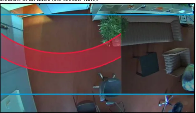
The cameras and sensors are placed in the IoTap lab located in Niagara, Malmö University. The lab has two entrances, which are both monitored by two cameras, one camera by each entrance. The cameras monitor the people going in and out of the room. The cameras have two red lines (see Figure 2 and Figure 3) that trigger upon a person crossing - and as a result, a new event is triggered and sent to the database. The camera software can estimate current occupancy in the room based on the number of people going in and out. Each time a person leaves or enters the room, an event is triggered - this event triggers a lambda function in Amazon Web Services (AWS, what we refer to as our database) to update the person count in the room. The person count (occupancy) is used as ground truth for the sensor data that is being used to train the DL networks. Temperature, humidity, light level and air pressure are collected by sensors which update their own respective table in the database continuously. A relay center on an Android device is also used for manually updating current occupancy in the room. Because the occupancy count is not accurate at all times (see section 4.2.1).

Figure 2. A picture captured from one of the camera sensors, showing the red line which triggers an event upon anyone crossing

12

Figure 3. A picture captured from one of the camera sensors, showing the red line which triggers an event upon anyone crossing

4.2.1 Validating camera and dataset accuracy

The cameras use software called AXIS Occupancy Estimator, it is what estimates occupancy in the room based on triggering events as mentioned in the previous paragraph. An Axis representative performed camera tuning on February 27th, previous to the start of our data collection. To validate the accuracy of the cameras, we used their built-in tool for testing accuracy. However, the camera accuracy does not ensure the accuracy of the occupancy estimator. We performed random samples during the time we were present in the lab, within the three week period of collecting data. No pre-processing of the dataset such as normalisation or cross-validation have been applied to the dataset. Validation results can be found in section 5.4.

4.3 Implementation of methodology

In the following section, the implementation process of the design and creation methodology will be summarised to give an overview of what was done and achieved during each phase. The development and evaluation phases were completed as an iteration cycle, in order to try to improve the performance of each DL network.

4.3.1 Awareness

This phase was previously completed by the stakeholder for this study - the problem had already been identified beforehand.

13

4.3.2 Suggestion

A big part of this phase was previously completed by the stakeholder; the stakeholder had already defined which techniques and data that should be used in order to research the problem. We defined which tools we would use to be able to answer the research question; namely, a stable and robust programing language, DL networks and libraries related to the DL networks. We chose to use the programming language Python along with Tensorflow, due to the robustness in both of these. For the DL networks, we chose to specifically use CNN, DNN and LSTM in our study, due to CNN and LSTM being the most widely used DL networks in previous work, as per state of the art (see: section 3). DNN is used because it was the first DL network we applied our problem too, in order to attain knowledge of how Tensorflow works.

4.3.3 Development

Under the development phase, the design and functionality for each of the involved DL networks in the study were programmed. Each DL network followed the same structural way of building and was built in Python, using the Tensorflow library. We started with specifying how the DL network would process the data from the sensors. We decided to use Comma Separated Values (CSV) files to input the DL networks with data. All sensor readings and corresponding ground truth (number of people in the room) was matched by timestamps, and collected in one single file (see: section 5.1 for an example of dataset structure). A Python script was developed to bind together the values from each sensor that had the same timestamp. The paired values were stored in a CSV file, and this dataset was split into training data (70% of total data) and testing data (30% of total data), resulting in two separate CSV files. The training and testing data was split using random-split evaluation [22].

In the first iteration of the development phase, we built basic DL networks. The main goal with this iteration was to have DL networks that would be able to process how the sensor data was structured and to produce an output for us. Each iteration was done in a trial-and-error fashion. Namely, based on the feedback we gathered from the evaluation phase, hyperparameters (hidden layers, kernel size, batch size, epochs) were changed in the network in order to try to improve the performance. Previous research gave us indications on which hyperparameters we would tune, in order to try to produce the highest possible accuracy – see section 3.2.1, 3.2.2 and 3.2.3. When the hyperparameter was selected we decided an interval for each hyperparameter to tune. Within these intervals, we used a range of values to see how each hyperparameter behaved at different value levels. We tested only to change one hyperparameter at a time to easily distinguish how the specific hyperparameter affected the accuracy. Trough each new iteration a new value level was tested to see its impact on the performance. Once we had tested the

14

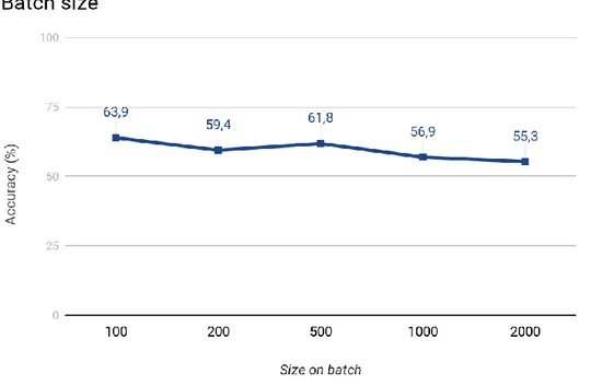
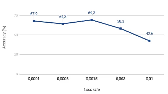
values within the ranges for the hyperparameters of the DL network, began we to make combinations out of those values that gave indications that these values together could produce a high predicate accuracy. This combination of values process was done in the final iterations. Surrounding values and other combinations were also tested. This whole work process was done for all the three (3) DL networks. Figures 4 to 8 illustrates how the work process for the LTSM went through. In the figures, the interval values are based on those values shown in Table 1 in the first iteration column for the LSTM network.

Table 1. First and final iteration for each DL network

Network First iteration Final iteration

CNN Batch size: 10 Kernel size: 5 Epochs: 100 Hidden units: 8 Learning rate: 0.00015 Batch size: 30 Kernel size: 5 Epochs: 200 Hidden units: 64 Learning rate: 0.0001 DNN Batch size: 10 Epochs: 100

Hidden units / layers: 5 units, 2 layers

Batch size: 100 Epochs: 1000

Hidden units / layers: 10 units, 2 layers LSTM Batch size: 100 Epochs: 100 Hidden units: 8 Learning rate: 0.0025 Loss rate: 0.0015 Batch size: 1500 Epochs: 400 Hidden units: 64 Learning rate: 0.0025 Loss rate: 0.0015

15

Figure 4. Illustrates the experimental process as the number of epochs was increased.

16

Figure 6. Illustrates the experimental process as the number of hidden units was increased.

17

Figure 8. Illustrates the experimental process as the loss rate was increased.

The training and testing of the DL networks and ML models were run solely on a MacBook Pro running macOS High Sierra, with an Intel Core i5 Processor at 2.7 GHz and 8GB RAM. Due to Tensorflow is restricted to solely using the central processing unit (CPU) for this computer, this is taken into consideration when running the training and testing of the DL networks. The hardware specifications were also taken into consideration when developing the DL networks. Because the hardware specifications have its limitations of how much it could much workload it can handle and thus limit us. It limited us in the way of restricting us to not choose values for the hyperparameters that would result in enormous training and testing running time. Not be able to choose these values could possibly have resulted in better produced predictive accuracies for the DL networks.

4.3.4 Evaluation

After finishing development of the necessary functionality for each DL network, the accuracy of how well it could make the right ground truth predictions were tested. If the tested network performed inconsistently (i.e. one network producing a predictive accuracy that is vastly different from the other networks, e.g. figuratively, CNN producing a predictive accuracy of 20%, but LSTM producing a predictive accuracy of 80% on the same dataset), the network was taken back to the development phase to be improved. For each DL network, there is a number of hyperparameters that can be changed in order to improve the accuracy. These hyperparameters can be the number of hidden layers, the batch size, the kernel size, how many training iterations or

18

the number of neurons in the hidden layers. Evaluation of which hyperparameters were changed was made in a trial-and-error.

4.3.5 Conclusion

This chapter will be thoroughly discussed in section 8.

4.4 Method discussion

Experiment or any modified form of experiments, e.g. quasi-experiments can be seen as an alternative research methodology for this study, instead of design and creation. Experiments could have been used instead since the experiment takes place in a controlled environment. However, it is known that the cameras registering events upon people entering and leaving the room does not always calculate the expected occupancy. We supervised the correctness by taking cluster samples from the database at times when we were working in the room, to verify that the right number of people was registered in the database. The other sensors are harder to verify correctness since we did not have the necessary tools to measure any of the sensor readings ourselves.

For our data generation, we used observation as the method, and we consider it to be the only reasonable approach to use for this study. We consider it to be the only reasonable approach because of no other type of data generation method e.g survey, documentation or questionnaire can generate this type of data that we need. Also, it would not be possible for the data generation methods to be able to produce the same amount of data that observation can do in such short time period that we have. We decided to use an iterative cycle between the development and evaluation phase since it would benefit how we approached the trial-and-error of improving performance for the DL networks.

5 Results

5.1 Dataset

During the data generation period, which lasted during the span of three weeks - from 12:30 March 8th 2018 to 12:30 March 29th 2018, a total of 31287 entries were combined into our final dataset. These entries were downloaded from our database and stored in a single CSV file. This CSV file contains what we refer to as our total data. The total data was split into two CSV files, the first containing 70% of the total data and the second 30% of the total data, of which we refer to as training and testing data, respectively. The training data (70% of total data) contains 21906 entries, while the testing data (30% of total data) contains 9381 entries. An example of how the dataset was

19

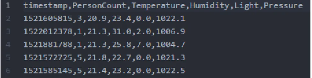
structured can be seen in Figure 9, each row contains a timestamp, the ground truth of the number of people in the room (occupancy), current temperature, current humidity, current light and current pressure.

Figure 9. Excerpt depicting the structure of the dataset

5.2 Deep learning

In this section, the predictive accuracy for the tested DL networks is presented. We will also describe in detail how the DL networks are structured. See Table 2 for an overview of the produced accuracy rates for each DL network and ML approach. The following sections require a brief introduction to certain keywords (see: keywords after table of contents).

Table 2. Overview of the produced predictive accuracy for all the approaches (DL and ML)

Network LSTM CNN DNN Gini Entrop

y

Accuracy 78.2 % 45.6 % 40.3 % 61.3 % 57.2 %

5.2.1 DNN

Our DNN network uses a DNN classifier from the Tensorflow library. The DNN classifier makes computations in the back-end of the library, we only have to define how data is processed by the network. We also had to define hyperparameters: the number of hidden layers and how many neurons each hidden layer consisted of, how many input and output neurons the networks would consist of, how many epochs training was run for. For our DNN, we had four (4) neurons in our input layer, each input neuron represented one of the sensor modalities. We used two (2) hidden layers with ten (10) neurons in each hidden layer. In our output layer, we set the number of neurons to 19 because the highest person count in our recorded data is 18 (range from 0-18). See Figure 10 for a visual representation of the structure. We trained our DNN network for 100 epochs with a batch size of 1000 shuffled samples, e.g. for each training round, 1000 shuffled data samples were run by the DNN network. The predictive accuracy for the DNN network was 40.3% with the specified structure and hyperparameters described.

20

Figure 10.. Shows the overall structure of the DNN network

5.2.2 LSTM/RNN

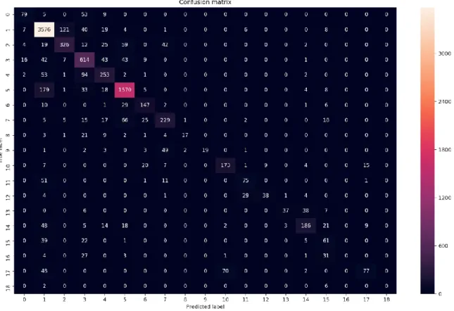
Our LSTM network is a modified RNN network, that has 2 LSTM memory cells that allow the network to retain information better. The LSTM network consists of five (5) layers, with one (1) input layer, one (1) hidden layer which contains 64 neurons, one (1) output layer and two (2) recurrent layers that act as the two LSTM (2) memory cells. Just like the output layer for the DNN network, the output layer for the LSTM network consists of 19 neurons. The input layer of the LSTM consists of 4 neurons. See Figure 11 for a visual representation of the structure for the network. Further, the network was run with a learning rate of 0.0025, a lambda loss rate of 0.0015. Linear activation with a Rectified Linear Unit (ReLU) was used, and softmax function applied. With this LSTM network structure, it produced a 68.3% accuracy rate by running the training for 200 epochs with a batch size of 1500 samples and a step size of 4. We increased the number of epochs from 200 to 400 and got an increased predictive accuracy. By running the training for 400 epochs, the LSTM network produced a 78.2% accuracy rate. Figure 12 depicts a confusion matrix for the predictions made with 78.2% accuracy rate.

21

Figure 12. Confusion matrix for the LSTM network

5.2.3 CNN

Our CNN network is built with the help of the Tensorflow library. The CNN network consists of six (6) different layers, with one (1) input layer, two (2) convolutional layers, one (1) pooling layer, one (1) fully connected layer and one (1) softmax layer. The input layer is structured as a 150x1 matrix, with a window size of 150. The first 1D (one-dimensional) convolution layer has a filter size and a depth of ten (10), followed by the max-pooling layer. The 1D max-pooling layer has a filter size of 20 and is followed by the second 1D convolution layer, which has a filter size of six (6). The fully connected layer consists of 64 neurons and connects to a softmax layer. The output layer consists of 19 labels (range of 0-18). Further, the specified kernel size is 5 and depth is 10. Learning rate is set to 0.0001. See Figure 13 for a visual representation of the structure for the network. With this structure for the CNN network, we achieved a 45.6% predictive accuracy rate by running the training for 100 epochs with a batch size of 30 samples.

22

Figure 13. Shows the overall structure of the CNN network

5.3 Traditional approach

5.3.1 Decision tree

We used decision trees as our traditional approach. Two types of decision tree formulae were used: Gini and Entropy. We used the same data for our decision trees as for our DL networks. The Gini formulae produced a predictive accuracy rate of 61.3%, while the Entropy formulae produced a predictive accuracy rate of 57.2%.

5.4 Camera and dataset accuracy

To make an estimation on the accuracy of the occupancy (our ground truth value), we prepared a full day where we recorded the current occupancy value and the real occupancy value, set apart with approximate 5 minute spans, or upon people entering or leaving the room. If the collected ground truth value was different from the real ground truth value, the current ground truth value was set to match the real value; e.g. 4 people supposedly in the room when there was actually 5, then the counter was set to 5. The entry was also flagged as erroneous.

During the day, there was a moderate activity of people entering and leaving the room. The maximum real value was 8, and the minimum real value was 0. The maximum estimated value was 7, and the minimum estimated value was 0. We started taking samples at 10:10, and stopped taking samples at 15:45. During this time, 66 sample entries were collected. Out of the entries, 18 were erroneous entries. This gives us an estimated accuracy of 72.72%. This estimated accuracy refers to the percentage of times the occupancy count was correct. We noticed that in cases where people entered at the same time or left at the same time, in certain cases the camera would only register the event as one person leaving; thus, making the occupancy counter show an incorrect value in respect to the real value. Since the test is performed using the same approach, in terms of estimating occupancy, as when our dataset was collected, we are able to make an estimation on how accurate the ground truth

23

value was during the data collection period. One thing to note is that the estimation corresponds to time between regular working hours (08:00 to 16:00), as for data outside of this time period - see section 7.1.

6 Analysis

6.1 Analysis of the dataset

The measured temperature values in the dataset were in a range between 23.5 ℃ as the highest temperature and 20.5 ℃ as the lowest temperature. The temperature difference for the total dataset was 3.5 ℃. See Table 3 for average, median and min, max values for all measured sensor modalities.

Table 3. Shows the mean, median, min, max values, range and mode for the measured sensor modalities.

Person count

Pressure Light Humidity Temperatu re Mean 4.2 1006.4 hPa 2614.6 lux 27.8 % 21.6 ℃ Median 3.0 1006.5 hPa 2.0 lux 28.7 % 21.4 ℃ Max value 18.0 1023.1 hPa 65531.0 lux 35.3 % 23.5 ℃ Min value 0.0 988.7 hPa 0.0 lux 19.5 % 20.5 ℃

Range 18.0 34.4 hPa 65531.0

lux 15.8 % 3.0 ℃

Mode 1.0 1004,8

hPa

2.0 lux 26.9 % 21.3 ℃

18 people were the highest number of people that the camera estimated occupancy to be in the room at the same time. During this time, when these individuals resided in the room, the measured sensor modalities were registered as in Table 4. During periods where the room was empty, the measured sensor modalities were registered as in Table 5.

Table 4. Shows average values for the measured sensor modalities when occupancy was n=18

Person count Pressure Light Humidity Temperature

24

Table 5. Shows average values for the measured sensor modalities when the room was empty (occupancy n=0)

Person count Pressure Light Humidity Temperature

0.0 997.4 hPa 2466.4 lux 28.4% 22.0 ℃

The Arduino sensor measured the highest temperature in the room to be 23.5 ℃ during the three-week observation. See Table 6 for the other measured sensor modalities that was measured during the same time as the highest temperature was measured. See Table 7 for the measured sensor modalities when the lowest temperature was measured.

Table 6. Shows average values for other measured sensor modalities during highest temperature measurement

Person count Pressure Light Humidity Temperature

5.0 1011.7 hPa 65531.0 lux 24.8% 23.5 ℃

Table 7. Shows average values for other measured sensor modalities during lowest temperature measurement

Person count Pressure Light Humidity Temperature

5.0 1003.5 hPa 1619.7 lux 22.6 % 20.5 ℃

The Arduino sensor measured the highest pressure in the room to be 1023.1 hPa during the three-week observation. During the same time span, the sensor also measured the lowest pressure in the room to be 988.7 hPa. See Table 8 for the other measured sensor modalities during the same time as the highest pressure was measured. See Table 9 for the other measured sensor modalities when the lowest pressure was measured.

Table 8. Shows average values for other measured sensor modalities during highest pressure measurement

Person count Pressure Light Humidity Temperature

6.0 1023.1 hPa 0.0 lux 23.4 % 21.2 ℃

Table 9. Shows average values for other measured sensor modalities during lowest pressure measurement

Person count Pressure Light Humidity Temperature

25

The Arduino sensor measured the highest humidity in the room to be 35.3% during the three-week observation. During the same time span, the sensor also measured the lowest humidity to be 19.5%. See Table 10 for the other measured sensor modalities during the same time as the highest humidity was measured. See Table 11 for the other measured sensor modalities when the lowest humidity was measured.

Table 10. Shows average values for other measured sensor modalities during highest humidity measurement

Person count Pressure Light Humidity Temperature

26

Table 11. Shows average values for other measured sensor modalities during lowest humidity measurement

Person count Pressure Light Humidity Temperature

5.0 1007.1 hPa 65531.0 lux 19.5 % 22.1 ℃

The Arduino sensor recorded the highest light level in the room to be 65531 lux during the three-week observation. During the same time span, the sensor also measured the lowest light level to be 0 lux. See Table 12 for the other sensor modalities that was recorded during the same time as the highest humidity was measured. See Table 13 for the other measured sensor modalities when the lowest humidity was measured.

Table 12. Shows average values for other measured sensor modalities during highest light level measurement

Person count Pressure Light Humidity Temperature

4.0 1006.3 hPa 65531.0 lux 27.8 % 21.8 ℃

Table 13. Shows average values for other measured sensor modalities during lowest light level measurement

Person count Pressure Light Humidity Temperature

6.0 1004.8 hPa 0.0 lux 28.7 % 21.4 ℃

6.2 Analysis of DL networks performance

In Table 2, we can see the results of each network’s performance and their resulting predictive accuracy on the dataset - from this table, we can see that the LSTM network outperforms the other approaches on our dataset. The LSTM approach has a predictive accuracy of 78.2%. The other DL approaches, DNN and CNN, perform similarly to each other - at 40.3% and 45.6% respectively. The traditional ML approaches, Entropy and Gini, perform similarly to each other - at 57.2% and 61.3% respectively. ML approaches seem to outperform DNN and CNN approaches, this might suggest that the data is linear and a simple classifier can classify better than the above-mentioned DL approaches. Entropy produced a predictive accuracy of 57.2%, 11.6 pp above the predictive accuracy for CNN, 16.9 pp above the predictive accuracy for DNN, and 21 pp below the predictive accuracy for LSTM. Gini produced a predictive accuracy of 61.3%, 15,7 pp above the predictive accuracy for CNN, 21 pp above the predictive accuracy for DNN, and 16.9 pp below the predictive accuracy for LSTM. LSTM, the best performing network,

27

produced a predictive accuracy of 78.2%, 32,6 pp above the predictive accuracy for CNN, and 37,9 pp above the predictive accuracy for DNN. The predictive accuracy produced by the LSTM might suggest that the memory-like cells in the network can pertain valuable information.

28

7 Discussion

The result of this study shows that out of the three (3) DL networks included in this study, only the LSTM network was able to produce a higher predictive accuracy than the traditional ML approaches. This result does not necessarily mean that deep learning approaches in general are able to produce a higher predictive accuracy than traditional machine learning approaches. However, the result can give indications for future work or evidence that deep learning approaches can produce a higher predictive accuracy than traditional ML approaches.

7.1 Dataset accuracy

Some results from the analysis of the dataset raise questions about how credible the sensor readings are. The fact that the light level in the room would reach up 65531 lux is one factor that raises questions regarding the credibility. Direct sunlight is approximated to be 100000 lux meanwhile, daylight is approximated to be 10000 lux [33]. A possible factor to the high light level recorded can be caused by the placement of the sensor that was measuring current light level in the room. The placement of the sensor might have allowed the sunlight to be directed to the lens of the sensor, thus allowing the high value of light to be recorded. Another question that raises questions regarding the dataset accuracy is how the values relate to each other, particularly the temperature and the person count values. The dataset shows that the room had the same temperature value at 22.0 ℃ when the room was occupied with the highest number people recorded (18 people) and with the lowest number of people in the room (0 people). The room was also warmer when a total of five (5) people occupied the room (23.5 ℃), compared to when 18 people occupied the room (22.0 ℃). These occurrences can possibly be explained by climate control. However, there is no big difference between the temperature values for these occurrences. This can indicate that the climate control works as intended, it levels the temperature to a pleasant temperature for these different occasions when a different number of people occupied the room. It is not possible to control when the climate control is activated and when it is not, which leads to uncertainty about the underlying cause. However, the average person count (4.2 people) suggests that the dataset is reasonably accurate - which is reasonable in comparison to the times we were in the room to validate the person count. The median (3 persons) for the person count also suggests that the accuracy of the dataset is reasonably accurate, in accordance with samples taken.

Unfortunately, the cameras were set to register events throughout the entire day, from 00:00 to 00:00. As per Figure 14 and the camera manual “The application automatically disables the counting functionality when it gets dark.” [32], this suggests that our dataset might be prone to erroneous data.

29

Having two cameras with two entrances might also lead to inaccuracy due to people registering in and out events using different entrances, thus resulting in an inaccurate occupancy count. Having heavily supervised ground truth data would be a sufficient way to mitigate this issue. This should be addressed in future work.

Figure 14. Warning message in AXIS Occupancy Estimator

7.2 Model selection

Model selection for HAR-related tasks can be difficult. There is no consensus on which model fits HAR best, and there is certainly no “one-model-fits-all”. Each implementation of a model is contextually dependent on the task at hand - e.g. a CNN that classifies irises is likely not suitable to classify movement from a gyroscope or accelerometer data. Model types that have been selected for HAR-related tasks, as per [1], include: DNNs, CNNs, RNNs, Stacked Autoencoders (SAE), Deep Belief Networks (DBN), Restricted Boltzmann Machines (RBM), and hybrid models (combinations of different DL-models). We chose to limit our model selections to three DL-models and one traditional approach partly due to time constraints, but also due to previous research has widely evaluated CNN, RNN and DNN models in the context of HAR - as seen in [1, Table. 4]. In the context of our research question, only three models are included and thus does not provide a big coverage of deep learning approaches. Introducing other approaches can bring interesting discussions on which approach is best practice for given task.

7.3 Model tuning

In line with previous studies, our LSTM did perform better than the CNN model in classifying occupancy. This is consistent with what has been found in previous studies on general HAR-related tasks. Previous studies have demonstrated that performance depends heavily on fine-tuning DL networks [17], [18]; our result ties well with this premise, and arguably our models could be tweaked further. The CNN and DNN models produced a significantly lower accuracy than the LSTM model did - this could be a due to human error in regards to programming, or a wrong interpretation of how these models function.

30

7.4 Potential factors affecting results

Potential factors that we think can have affected the results are as follows: 1. Climate control - As previously stated, the observed room, like all public

spaces in Niagara, is under climate control - meaning that the building controls parameters such as temperature and relative humidity. In regard to our thesis, this is a major limitation, as the variance in data will be inconsistent.

2. Skills of us developers - We set into this thesis and subject with no prior experience; there are many aspects that could impact the results, not limited to:

a. Programming skills, building complex models and computer - Even though we have attained knowledge of other programming languages, our expertise in Python remains scarce. This was our first time implementing anything in Python, and starting with a huge library such as Tensorflow is indeed a challenge. Expanding on model implementations, building deep learning models such CNN, DNN and LSTM models proved to be complex. It was not only hard to grasp - but also to fully understand, especially when mathematics and statistics were involved. The training and testing of the DL networks were run solely on a CPU, not a GPU-accelerated computer, which could have an impact on the results - limited hardware specifications lead to the training and testing of each network to take a longer time. By using a computer with better hardware specifications it would have allowed us to try higher values on the hyperparameters, since it took a long time to run the training and testing process.

b. Knowledge of the subject - Our knowledge in the subject of HAR, DL and ML were non-existent previous to this thesis. All experience in relation to concepts revolving around these subjects has been attained in a short amount of time, and could possibly be a culprit of any mishaps.

3. Time allocation - We think now at the end of the study, that it would be wiser to only focus on one single DL approach, due to the added complexity of having to develop multiple deep learning approaches with no prior knowledge. We spent a lot of time figuring out technicalities of each approach; when perhaps if time had been allocated to one approach, we might have been able to produce a well-adjusted fine-tuned model.

The main conclusion that can be drawn from the study is that DL approaches have the ability to produce a higher predictive accuracy than traditional ML

31

approaches. Further comparisons need to be made, in order to validate how efficient DL approaches are for HAR using sensor data.

32

8 Conclusion

In this thesis, we compare the predictive accuracy of three deep learning models to the predictive accuracy produced by traditional methods, on our presented dataset. Compared to traditional methods, one class of deep learning networks perform better on our dataset. Our LSTM network achieves the best performance out of all approaches, in classifying occupancy based on sensor readings from our smart office. Finally, possible future works within the field are presented in the following section.

8.1 Future work

This section is dedicated to presenting future work, based on the progress made in this thesis. There are several challenges yet to explore:

1. Further experimentation with dataset and hyperparameters - Tweaking the hyperparameters to a better extent might prove beneficial in terms of performance. Although this thesis tries to produce high performance, well-adjusted models, it is likely that more adjustment can impact the performance of each model. Testing the same dataset with a different partitioning of training and testing data might also prove beneficial, e.g. running experiments with 90% training data and 10% testing data, or other combinations of partitioning - perhaps using cross-validation. 2. Gather more data and properly validate the data - As our dataset is not

huge, it could be crucial for the performance of all models if the dataset was larger. Deep learning models often require large datasets for

optimal performance. Validation of data (properly annotated data) and erroneous data would strengthen the validity of the study.

3. Comparison to other deep learning and machine learning approaches - Our thesis compares three deep learning approaches and one machine learning approach. Expanding on these approaches, but also

introducing different approaches can bring interesting results on which approach is best suited for the purpose.

33

References

[1] J. Wang, Y. Chen, S. Hao, X. Peng, och L. Hu, ”Deep Learning for Sensor-based Activity Recognition: A Survey”, Pattern Recognition Letters, February 2017.

[2] Y. Bengio, ”Deep Learning of Representations: Looking Forward”,

arXiv:1305.0445 [cs], May 2013.

[3] O. D. Lara och M. A. Labrador, ”A Survey on Human Activity Recognition using Wearable Sensors”, IEEE Communications Surveys Tutorials, vol. 15, no 3, pp. 1192–1209, March 2013.

[4] P. A. Jarvis, T. F. Lunt, och K. L. Myers, ”Identifying Terrorist Activity with AI Plan Recognition Technology”, AI Magazine, vol. 26, no 3, pp. 73, September 2005.

[5] M. E. Pollack, ”Intelligent Technology for an Aging Population: The Use of AI to Assist Elders with Cognitive Impairment”, AI Magazine, vol. 26, no 2, pp. 9, June 2005.

[6] J. R. Kwapisz, G. M. Weiss, and S. A. Moore, ‘Activity Recognition Using Cell Phone Accelerometers’, SIGKDD Explor. Newsl., vol. 12, no. 2, pp. 74–82, Mar. 2011.

[7] W. H. Chen, C. A. B. Baca, and C. H. Tou, ‘LSTM-RNNs combined with scene information for human activity recognition’, in 2017 IEEE 19th

International Conference on e-Health Networking, Applications and Services (Healthcom), 2017, pp. 1–6.

[8] S. Münzner, P. Schmidt, A. Reiss, M. Hanselmann, R. Stiefelhagen, and R. Dürichen, ‘CNN-based Sensor Fusion Techniques for Multimodal Human Activity Recognition’, in Proceedings of the 2017 ACM International Symposium

on Wearable Computers, New York, NY, USA, 2017, pp. 158–165.

[9] Y. Guan and T. Plötz, ‘Ensembles of Deep LSTM Learners for Activity Recognition Using Wearables’, Proc. ACM Interact. Mob. Wearable Ubiquitous

Technol., vol. 1, no. 2, p. 11:1–11:28, Jun. 2017.

[10] D. Singh, E. Merdivan, S. Hanke, J. Kropf, M. Geist, and A. Holzinger, ‘Convolutional and Recurrent Neural Networks for Activity Recognition in Smart Environment’, in Towards Integrative Machine Learning and Knowledge