Article
Combining Multiconfiguration and Perturbation
Methods: Perturbative Estimates of Core–Core
Electron Correlation Contributions to Excitation
Energies in Mg-Like Iron
Stefan Gustafsson1, Per Jönsson1,*, Charlotte Froese Fischer2and Ian Grant3,4 1 Materials Science and Applied Mathematics, Malmö University, SE-205 06 Malmö, Sweden;
stefan.gustafsson@mah.se
2 Department of Computer Science, University of British Columbia, Vancouver, BC V6T 1Z4, Canada;
charlotte.f.fischer@comcast.net
3 Mathematical Institute, University of Oxford, Woodstock Road, Oxford OX2 6GG, UK;
iangrant15@btinternet.com
4 Department of Applied Mathematics and Theoretical Physics, Centre for Mathematical Sciences,
Wilberforce Road, Cambridge CB3 0WA, UK
* Correspondence: per.jonsson@mah.se; Tel.: +46-40-66-57251 Academic Editor: Joseph Reader
Received: 25 November 2016; Accepted: 6 January 2017; Published: 12 January 2017
Abstract:Large configuration interaction (CI) calculations can be performed if part of the interaction is treated perturbatively. To evaluate the combined CI and perturbative method, we compute excitation energies for the 3l3l0, 3l4l0and 3s5l states in Mg-like iron. Starting from a CI calculation including valence and core–valence correlation effects, it is found that the perturbative inclusion of core–core electron correlation halves the mean relative differences between calculated and observed excitation energies. The effect of the core–core electron correlation is largest for the more excited states. The final relative differences between calculated and observed excitation energies is 0.023%, which is small enough for the calculated energies to be of direct use in line identifications in astrophysical and laboratory spectra.
Keywords:excitation energies; multiconfiguration Dirac–Hartree–Fock; configuration interaction
1. Introduction
Transitions from highly charged ions are observed in the spectra of astrophysical sources as well as in Tokamak and laser-produced plasmas, and they are routinely used for diagnostic purposes [1]. Often, transitions between configurations in the same complex are used, but transitions from higher lying configurations are also important (see, e.g., [2] for a discussion of the higher lying states in the case of Mg-like iron). Transition energies are available from experiments for many ions and collected in various data bases [3], but large amounts of data are still lacking. Although experimental work is aided by a new generation of light sources such as EBITs [4], spectral identifications are still a difficult and time-consuming task. A way forward is provided by theoretical transition energies that support line identification and render consistency checks for experimental level designations.
Much work has been done to improve both multiconfiguration methods and perturbative methods, each with their strengths and weaknesses, in order to provide theoretical transition energies of spectroscopic accuracy, i.e., transition energies with uncertainties of the same order as the ones obtained from experiments and observations using Chandra, Hinode or other space based missions in the X-ray and EUV spectral ranges [5–8]. Further advancements for complex systems with several
electrons outside a closed atomic core calls for a combination of multiconfiguration and perturbative methods [9] and also for methods based on new principles [10,11].
In this paper, we describe how the multiconfiguration Dirac–Hartree–Fock (MCDHF) and relativistic configuration interaction (CI) methods can be modified to include perturbative corrections that account for core–core electron correlation. Taking Mg-like iron as an example, we show how the corrections improve excitation energies for the more highly excited states.
2. Relativistic Multiconfiguration Methods
2.1. Multiconfiguration Dirac–Hartree–Fock and Configuration Interaction
In the MCDHF method [12,13], as implemented in the GRASP2K program package [14], the wave functionΨ
(
γP J MJ)
for a state labeled γPJ MJ, where J and MJare the angular quantum numbers and P is the parity, is expanded in antisymmetrized and coupled configuration state functions (CSFs)Ψ(γP J MJ
) =
M∑
j=1
cjΦ(γjPJ MJ
).
(1)The labels
{
γj}
denote other appropriate information of the configuration state functions, such as orbital occupancy and coupling scheme. The CSFs are built from products of one-electron orbitals, having the general formψnκ,m
(
r) =
1 r Pnκ(r)
χκ,m(
θ, ϕ) ıQnκ(r)
χ−κ,m(
θ, ϕ)
! , (2)where χ±κ,m
(
θ, ϕ)are 2-component spin-orbit functions. The radial functions{P
nκ(r), Q
nκ(r)}
are numerically represented on a grid.Wave functions for a number of targeted states are determined simultaneously in the extended optimal level (EOL) scheme. Given initial estimates of the radial functions, the energies E and expansion coefficients c
= (c
1, . . . , cM)
t for the targeted states are obtained as solutions to the configuration interaction (CI) problemHc
=
Ec, (3)where H is the CI matrix of dimension M
×
M with elementsHij
= hΦ(
γiPJ MJ)|H|Φ(
γjPJ MJ)i.
(4) In relativistic calculations, the Hamiltonian H is often taken as the Dirac–Coulomb Hamiltonian. Once the expansion coefficients have been determined, the radial functions are improved by solving a set of differential equations results from applying the variational principle on a weighted energy functional of the targeted states together with additional terms needed to preserve orthonormality of the orbitals. The CI problem and the solution of the differential equations are iterated until the radial orbitals and the energy are converged to a specified tolerance.The MCDHF calculations are often followed by CI calculations where terms representing the transverse photon interaction are added to the Dirac-Coulomb Hamiltonian and the vacuum polarization effects are taken into account by including the Uehling potential. Electron self-energies are calculated with the screened hydrogenic formula [12,15]. Due to the relative simplicity of the CI method, often much larger expansions are included in the final CI calculations compared to the MCDHF calculations.
2.2. Large Expansions and Perturbative Corrections
The number of CSFs in the wave function expansions depend on the shell structure of the ionic system as well as the model for electron correlation (to be discussed in Section3). For accurate calculations, a large number of CSFs are required, leading to very large matrices. To handle these large matrices, the CSFs can a priori be divided into two groups. The first group, P, with m elements (m
M) contains CSFs that account for the major parts of the wave functions. The second group, Q, with M
−
m elements contains CSFs that represent minor corrections. Allowing interaction between CSFs in group P, interaction between CSFs in group P and Q and diagonal interactions between CSFs in Q gives a matrixH(PP) H(PQ) H(QP) H(QQ)
!
, (5)
where H(QQ)ij
=
δijEQi . The restriction of H(QQ)to diagonal elements results in a huge reduction in the total number of matrix elements and corresponding computational time. The assumptions of the approximation and the connections to the method of deflation in numerical analysis are discussed in [13]. This form of the CI matrix, which has been available in the non-relativistic and relativistic multiconfiguration codes for a long time [16,17], yields energies that are similar to the ones obtained by applying second-order perturbation theory (PT) corrections to the energies of the smaller m×
m matrix. The method is therefore referred to here as CI combined with second-order Brillouin–Wigner perturbation theory [18]. Note, however, that the CI method with restrictions on the interactions gives, in contrast to ordinary perturbative methods, wave functions that can be directly used to evaluate expectation values such as transition rates.3. Calculations
Calculations were performed for states belonging to the 3s2, 3p2, 3s3d, 3d2, 3s4s, 3s4d, 3p4p, 3p4 f , 3d4s, 3d4d, 3s5s, 3s5d, 3s5g even configurations and the 3s3p, 3p3d, 3s4p, 3p4s, 3s4 f , 3p4d, 3d4p, 3d4 f , 3s5p, 3s5 f odd configurations of Mg-like iron. For 3d4 f , only states below the 3p5s configuration were included. The above configurations define the multireference (MR) for the even and odd parities, respectively. Following the procedure in [19], an initial MCDHF calculation for all even and odd reference states was done in the EOL scheme. The initial calculation was followed by separate calculations in the EOL scheme for the even and odd parity states. The MCDHF calculations for the even states were based on CSF expansions obtained by allowing single (S) and double (D) substitutions of orbitals in the even MR configurations to an increasing active set of orbitals. In a similar way, the calculations for the odd states were based on CSF expansions obtained by allowing single (S) and double (D) substitutions of orbitals in the odd MR configurations to an increasing active set of orbitals. To prevent the CSF expansions from growing unmanageably large and in order to obtain orbitals that are spatially localized in the valence and core–valence region, at most, single substitutions were allowed from the 2s22p6core. The 1s2shell was always closed. The active sets of orbitals for the even and odd parity states were extended by layers to include orbitals with quantum numbers up to n
=
8 and l=
6, at which point the excitation energies are well converged.To investigate the effects of electron correlation, three sets of CI calculations were done. In the first set of CI calculations, one calculation was done for the even states and one calculation for the odd states, the SD substitutions were only allowed from the valence shells of the MR, and the CSFs account for valence–valence correlation. In the second set of calculations, SD substitutions were such that there was at most one substitution from the 2s22p6core, and the CSFs account for valence–valence and core–valence correlation. In the final set of calculations, all SD substitutions were allowed, and the CSFs account for valence–valence, core–valence and core–core correlation. When all substitutions are allowed, the number of CSFs grows very large. For this reason, we apply CI with second-order perturbation corrections. The CSFs describing valence–valence and core–valence effects (SD substitutions with at most one substitution from the 2s22p6core) were included in group P,
whereas the CSFs accounting for core–core correlation (D substitutions from 2s22p6) were included in group Q and treated in second-order perturbation theory. The number of CSFs for the different CI calculations are given in Table1.
Table 1. Number of CSFs for the even and odd parity expansions for the different sets of CI calculations. VV are the expansions accounting for valence–valence correlation, VV+CV are the expansions accounting for valence–valence and core–valence correlation and VV+CV+CC are the expansions accounting for valence-valence, core–valence and core–core correlation.
VV VV+CV VV+CV+CC
even 2738 644,342 5,624,158 odd 2728 630,502 6,214,393
4. Results
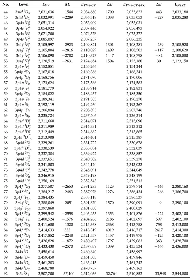
The excitation energies from the different CI calculations, along with observed energies from the NIST database [3], are displayed in Table2. From the table, we see that states belonging to 3l3l0, with the exception of 3s3p3P0,1,2, are too high for the valence–valence correlation calculation. The states belonging to 3l4l0 and 3s5l, on the other hand, are too low. When including also the core–valence correlation, the states belonging to 3l3l0go down in energy and approach the observed excitation energies. The states belonging to 3l4l0 and 3s5l go up and are now too high. Including also the core–core correlation results in a rather small energy change for the states belonging to 3l3l0. The main effect of the core–core correlation is to lower the energies of the states belonging to 3l4l0and 3s5l, bringing them in very good agreement with observations. The labeling of levels is normally done by looking at the quantum designation of the leading component in the CSF expansion [20]. There are two levels (67 and 69) with 3p4d3D3as the leading component in the corresponding CSF expansion. To distinguish these levels, we added subscripts A and B to the labels of the dominant component. In a similar way, subscripts A and B were added to distinguish levels 78 and 80, both with 3p4 f 3F3as the leading component.
Table2indicates that there are a few states that are either misidentified or assigned with a label that is inconsistent with the labels of the current calculation. The observed energy for 3p4 f3D2(level 84) is 2417 cm−1too low compared to the calculated value and the observed energy for 3s5s3S1(level 92) is 33,948 cm−1too high. There seem to be no other computed energy levels that match the observed energies. The observed energy for 3s5p1P1o (level 100) is 3733 cm−1 too low. The observed energy matches the computed energy of 3s5p3P1o(level 97), and, thus, it seems like an inconsistency in the labeling. Finally, 3s5 f 1Fo
3 (level 117) is 101,545 cm−1too high and there is no other computed energy level that matches. Removing the energy outliers above, the mean relative energy differences are, respectively, 0.217%, 0.051%, 0.023% for the valence, the valence and core–valence and the valence, core–valence and core–core calculations. The energy differences are mainly due to higher-order electron correlation effects that have not been accounted for in the calculations. At the same time, one should bear in mind that the observed excitation energies are also associated with uncertainties as reflected in the limited number of valid digits displayed in the NIST tables.
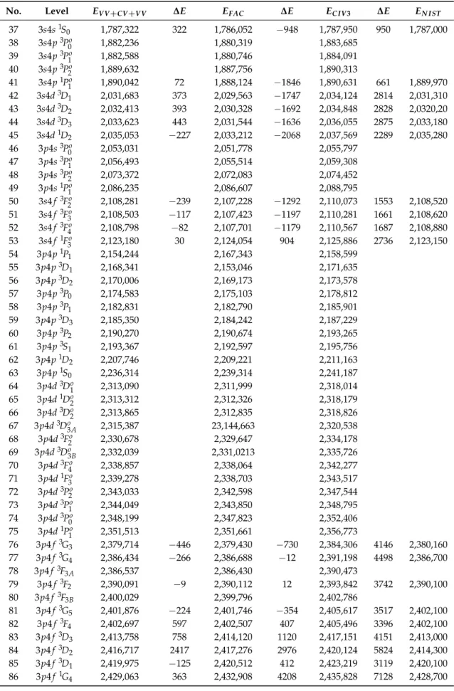
In Table3, the excitation energies obtained by including core–core correlation in the CI calculations are compared with energies from calculations by Landi [2] using the FAC code and with energies by Aggarwal et al. [21] using CIV3 in the Breit–Pauli approximation. The uncertainties of the excitation energies for the latter calculations are substantially larger. The calculations by Landi support the conclusion that some of the levels in the NIST database are misidentified. One may note that Landi gives levels 78 and 80 the labels 3p4 f3F3and 3p4 f 1F3, respectively, whereas Aggarwal et al. reverse the labels. This illustrates that labeling is dependent on the calculation and that the labeling process is far from straightforward [20].
Table 2.Comparison of calculated and observed excitation energies in Mg-like iron (Fe XV). EVVare
energies from CI calculations that account for valence–valence correlation. EVV+CVare energies from
CI calculations that account for valence–valence and core–valence electron correlation. EVV+CV+CCare
energies that account for valence–valence and core–valence electron correlation and where core–core electron correlation effects have been included perturbatively. EN ISTare observed energies from the
NIST database ([3]).∆E are energy differences with respect to EN IST. All energies are in cm−1.
No. Level EV V ∆E EV V +CV ∆E EV V +CV +CC ∆E EN IST
1 3s2 1S 0 0 0 0 0 0 0 0 2 3s3p3P0o 233,087 −755 233,828 −14 233,928 86 233,842 3 3s3p3Po 1 238,936 −724 239,668 8 239,741 81 239,660 4 3s3p3P2o 253,017 −803 253,829 9 253,773 −47 253,820 5 3s3p1P1o 354,941 3030 352,169 258 352,091 180 351,911 6 3p2 3P 0 556,594 2070 554,643 119 554,895 371 554,524 7 3p2 1D2 559,900 300 559,834 234 559,661 61 559,600 8 3p2 3P 1 566,524 1922 564,663 61 564,674 72 56,4602 9 3p2 3P2 583,327 1524 581,933 130 581,870 67 581,803 10 3p2 1S0 662,999 3372 660,269 642 660,229 602 659,627 11 3s3d3D1 680,522 1750 678,954 182 678,329 −443 678,772 12 3s3d3D2 681,520 1735 679,986 201 679,381 −404 679,785 13 3s3d3D 3 683,080 1664 681,603 187 680,952 −464 681,416 14 3s3d1D2 766,690 4597 762,729 636 762,176 83 762,093 15 3p3d3Fo 2 929,158 917 928,565 324 928,086 −155 928,241 16 3p3d3F3o 938,885 759 938,469 343 938,068 −58 938,126 17 3p3d1Do2 950,226 1713 948,768 255 948,383 −130 948,513 18 3p3d3F4o 950,300 642 949,990 332 949,451 −207 949,658 19 3p3d3Do1 986,221 3353 983,077 209 982,740 −128 982,868 20 3p3d3Po 2 986,499 2985 983,765 251 983,350 −164 983,514 21 3p3d3Do3 998,324 3472 995,088 236 994,712 −140 994,852 22 3p3d3Po 0 998,597 2708 996,218 329 995,835 −54 995,889 23 3p3d3P1o 999,166 2923 996,547 304 996,127 −116 996,243 24 3p3d3Do2 999,755 3132 996,892 269 996,449 −174 996,623 25 3p3d1F3o 1,066,906 4391 1,063,163 648 1,062,704 189 1,062,515 26 3p3d1P1o 1,078,913 4026 1,075,795 908 1,075,306 419 1,074,887 27 3d2 3F 2 1,373,374 3043 1,370,858 527 1,369,758 −573 1,370,331 28 3d2 3F3 1,374,983 2948 1,372,527 492 1,371,407 −628 1,372,035 29 3d2 3F4 1,376,965 2909 1,374,580 524 1,373,475 −581 1,374,056 30 3d2 1D2 1,405,702 3110 1,403,474 882 1,402,237 −355 1,402,592 31 3d2 3P0 1,409,066 1,406,328 1,405,381 32 3d2 3P1 1,409,639 1,406,926 1,405,672 33 3d2 1G4 1,409,702 2644 1,407,974 916 1,406,831 −227 1,407,058 34 3d2 3P 2 1,411,053 3280 1,408,467 694 1,407,210 −563 1,407,773 35 3d2 1S0 1,489,913 2859 1,488,993 1939 1,487,460 406 1,487,054 36 3s4s3S1 1,761,471 −2229 1,764,876 1176 17,63,699 −1 1,763,700 37 3s4s1S0 1,785,265 −1735 1,788,455 1455 1,787,322 322 1,787,000 38 3s4p3P0o 1,880,014 1,883,187 1,882,236 39 3s4p3Po 1 1,880,440 1,883,595 1,882,588 40 3s4p3P2o 1,887,508 1,890,703 1,889,632 41 3s4p1Po 1 1,887,872 −2098 1,891,051 1081 1,890,042 72 1,889,970 42 3s4d3D1 2,029,659 −1651 2,032,907 1597 2,031,683 373 2,031,310 43 3s4d3D2 2,030,413 −1607 2,033,653 1633 2,032,413 393 2,032,020
Table 2. Cont.
No. Level EV V ∆E EV V +CV ∆E EV V +CV +CC ∆E EN IST
44 3s4d3D3 2,031,636 −1544 2,034,880 1700 2,033,623 443 2,033,180 45 3s4d1D2 2,032,991 −2289 2,036,318 1038 2,035,053 −227 2,035,280 46 3p4s3Po 0 2,051,314 2,053,909 2,053,031 47 3p4s3P1o 2,054,922 2,057,446 2,056,493 48 3p4s3Po 2 2,071,700 2,074,376 2,073,372 49 3p4s1P1o 2,085,097 2,087,237 2,086,235 50 3s4 f3F2o 2,105,597 −2923 2,109,821 1301 2,108,281 −239 2,108,520 51 3s4 f3Fo 3 2,105,804 −2816 2,110,029 1409 2,108,503 −117 2,108,620 52 3s4 f3F4o 2,106,098 −2782 2,110,327 1447 2,108,798 −82 2,108,880 53 3s4 f1Fo 3 2,120,519 −2631 2,124,654 1504 2,123,180 30 2,123,150 54 3p4p1P1 2,152,851 2,155,266 2,154,244 55 3p4p3D1 2,167,018 2,169,386 2,168,341 56 3p4p3D2 2,168,756 2,171,070 2,170,006 57 3p4p3P0 2,173,624 2,175,566 2,174,583 58 3p4p3P 1 2,181,779 2,183,914 2,182,831 59 3p4p3D3 2,184,022 2,186,457 2,185,350 60 3p4p3P 2 2,189,341 2,191,385 2,190,270 61 3p4p3S1 2,192,119 2,194,460 2,193,367 62 3p4p1D2 2,206,894 2,208,893 2,207,746 63 3p4p1S0 2,235,724 2,237,406 2,236,314 64 3p4d3Do1 2,311,660 2,314,071 2,313,090 65 3p4d1Do 2 2,311,989 2,314,331 2,313,312 66 3p4d3Do2 2,312,449 2,314,882 2,313,865 67 3p4d3Do 3A 2,313,908 2,316,401 2,315,387 68 3p4d3F2o 2,329,261 2,331,722 2,330,678 69 3p4d3D3Bo 2,330,539 2,333,084 2,332,039 70 3p4d3F4o 2,337,384 2,339,922 2,338,857 71 3p4d1F3o 2,337,651 2,340,302 2,339,278 72 3p4d3Po 2 2,341,803 2,344,120 2,343,033 73 3p4d3P1o 2,342,778 2,345,091 2,344,049 74 3p4d3Po 0 2,346,915 2,349,198 2,348,199 75 3p4d1P1o 2,350,169 2,352,543 2,351,513 76 3p4 f3G3 2,377,507 −2653 2,381,283 1123 2,379,714 −446 2,380,160 77 3p4 f3G4 2,384,217 −2483 2,387,976 1276 2,386,434 −266 2,386,700 78 3p4 f 3F3A 2,384,435 2,388,118 2,386,537 79 3p4 f3F 2 2,388,049 −2051 2,391,670 1570 2,390,091 −9 2,390,100 80 3p4 f3F3B 2,397,860 2,401,630 2,400,029 81 3p4 f3G5 2,399,542 −2558 2,403,453 1353 2,401,876 −224 2,402,100 82 3p4 f3F4 2,400,524 −1576 2,404,286 2186 2,402,697 597 2,402,100 83 3p4 f3D3 2,411,680 −1320 2,415,368 2368 2,413,758 758 2,413,000 84 3p4 f3D 2 2,414,633 333 2,418,319 4019 2,416,717 2417 2,414,300 85 3p4 f3D1 2,417,852 −2248 2,421,557 1457 2,419,975 −125 2,420,100 86 3p4 f1G 4 2,426,828 −1872 2,430,497 1797 2,429,063 363 2,428,700 87 3p4 f1D2 2,433,430 −2570 2,437,039 1039 2,435,534 −466 2,436,000 88 3d4s3D1 2,458,614 2,460,640 2,458,997 89 3d4s3D2 2,459,450 2,461,503 2,459,846 90 3d4s3D3 2,461,283 2,463,415 2,461,742 91 3d4s1D 2 2,468,780 2,470,737 2,469,163 92 3s5s3S1 2,507,700 −37,100 2,512,036 −32,764 2,510,852 −33,948 2,544,800
Table 2. Cont.
No. Level EV V ∆E EV V +CV ∆E EV V +CV +CC ∆E EN IST
93 3s5s1S0 2,516,613 2,520,681 2,519,752 94 3d4p1Do2 2,561,358 2,563,408 2,561,899 95 3d4p3Do 1 2,564,069 2,567,301 2,565,949 96 3s5p3P0o 2,564,472 2,568,582 2,567,624 97 3s5p3Po 1 2,565,848 2,568,791 2,567,639 98 3d4p3Do2 2,567,134 2,569,092 2,567,703 99 3d4p3Do3 2,568,154 2,571,175 2,569,693 100 3s5p1Po 1 2,568,200 1200 2,571,834 4834 2,570,733 3733 2,567,000 101 3s5p3P2o 2,569,213 2,572,157 2,570,743 102 3d4p3Fo 2 2,570,296 2,572,316 2,571,126 103 3d4p3F3o 2,573,116 2,575,101 2,573,592 104 3d4p3Fo 4 2,576,139 2,578,374 2,576,829 105 3d4p3P1o 2,583,286 2,585,242 2,583,862 106 3d4p3P2o 2,583,400 2,585,407 2,583,960 107 3d4p3Po 0 2,583,734 2,585,658 2,584,322 108 3d4p1F3o 2,592,868 2,594,519 2,593,236 109 3d4p1Po 1 2,603,279 2,605,145 2,604,533 110 3s5d3D1 2,637,190 −2910 2,641,400 1300 2,640,247 147 2,640,100 111 3s5d3D2 2,637,419 −2481 2,641,630 1730 2,640,442 542 2,639,900 112 3s5d3D3 2,637,852 −2448 2,642,072 1772 2,640,870 570 2,640,300 113 3s5d1D2 2,639,773 2,643,981 2,642,888 114 3s5 f3Fo 2 2,672,676 −3724 2,677,360 960 2,675,889 −511 2,676,400 115 3s5 f3F3o 2,672,770 −3630 2,677,455 1055 2,675,988 −412 2,676,400 116 3s5 f3Fo 4 2,672,907 −3693 2,677,594 994 2,676,123 −477 2,676,600 117 3s5 f1F3o 2,678,041 −104,659 2,682,597 −100,103 2,681,155 −101,545 2,782,700 118 3s5g3G3 2,682,487 2,687,368 2,685,680 119 3s5g3G4 2,682,654 2,687,556 2,685,877 120 3s5g3G5 2,682,855 2,687,777 2,686,099 121 3s5g1G 4 2,685,580 2,690,506 2,688,841 122 3d4d1F3 2,699,116 2,701,602 2,699,874 123 3d4d3D 1 2,703,542 2,705,972 2,704,354 124 3d4d3D2 2,704,742 2,707,218 2,705,580 125 3d4d3D3 2,706,116 2,708,636 2,706,964 126 3d4d3G3 2,707,934 2,710,522 2,708,828 127 3d4d1P1 2,709,315 2,711,813 2,710,163 128 3d4d3G 4 2,709,360 2,711,928 2,710,264 129 3d4d3G5 2,711,220 2,713,878 2,712,174 130 3d4d3S1 2,720,698 2,723,175 2,721,783 131 3d4d3F2 2,726,309 2,728,092 2,726,350 132 3d4d3F3 2,727,568 2,729,398 2,727,634 133 3d4d3F 4 2,729,029 2,730,908 2,729,156 134 3d4d1D2 2,741,839 2,743,862 2,742,627 135 3d4d3P 0 2,744,213 2,746,022 2,744,706 136 3d4d3P1 2,744,807 2,746,626 2,745,163 137 3d4d3P2 2,745,935 2,747,809 2,746,300 138 3d4d1G4 2,748,985 2,751,121 2,749,474 139 3d4 f 3Ho4 2,765,833 2,770,098 2,768,443 140 3d4 f 1Go 4 2,767,533 2,771,821 2,770,030 141 3d4 f 3Ho5 2,767,692 2,771,943 2,770,434 142 3d4d1S 0 2,775,538 2,779,275 2,777,362
Table 2. Cont.
No. Level EV V ∆E EV V +CV ∆E EV V +CV +CC ∆E EN IST
143 3d4 f 3F2o 2,776,151 2,779,298 2,778,011 144 3d4 f 3F3o 2,776,264 2,779,933 2,778,867 145 3d4 f 3Fo
4 2,776,981 2,780,796 2,780,729
146 3d4 f1Do2 2,786,768 2,790,305 2,788,248
Table 3. Comparison of calculated and observed excitation energies in Mg-like iron (Fe XV). EVV+CV+CCare energies that account for valence–valence and core–valence electron correlation and
where core–core electron correlation effects have been included perturbatively. EFACare energies by
Landi [2] using the FAC code. ECIV3are energies by Aggarwal et al. [21] using the CIV3 code. EN IST
are observed energies from the NIST database ([3]).∆E are energy differences with respect to EN IST.
All energies are in cm−1.
No. Level EV V +CV +V V ∆E EFAC ∆E ECIV 3 ∆E EN IST
1 3s2 1S 0 0 0 0 0 0 0 0 2 3s3p3P0o 233,928 86 233,068 −774 235,013 1171 233,842 3 3s3p3P1o 239,741 81 238,900 −760 240,511 851 239,660 4 3s3p3P2o 253,773 −47 252,917 −903 253,548 −272 253,820 5 3s3p1P1o 352,091 180 356,126 4215 356,262 4351 351,911 6 3p2 3P 0 554,895 371 556,994 2470 560,275 5751 554,524 7 3p2 1D2 559,661 61 560,266 666 563,216 3616 559,600 8 3p2 3P 1 564,674 72 566,832 2230 569,295 4693 564,602 9 3p2 3P2 581,870 67 583,564 1761 584,856 3053 581,803 10 3p2 1S0 660,229 602 665,768 6141 665,260 5633 659,627 11 3s3d3D1 678,329 −443 680,146 1374 687,680 8908 678,772 12 3s3d3D2 679,381 −404 681,129 1344 688,733 8948 6797,85 13 3s3d3D 3 680,952 −464 682,667 1251 690,401 8985 681,416 14 3s3d1D2 762,176 83 769,369 7276 774,295 12,202 762,093 15 3p3d3Fo 2 928,086 −155 928,786 545 938,265 10,024 928,241 16 3p3d3F3o 938,068 −58 938,555 429 947,307 9181 938,126 17 3p3d1Do2 948,383 −130 949,447 934 958,402 9889 948,513 18 3p3d3F4o 949,451 −207 949,927 269 957,820 8162 949,658 19 3p3d3Do1 982,740 −128 986,082 3214 995,526 12,658 982,868 20 3p3d3Po 2 983,350 −164 986,407 2893 995,767 12,253 983,514 21 3p3d3Do3 994,712 −140 997,944 3092 1,007,026 12,174 994,852 22 3p3d3Po 0 995,835 −54 998,762 2873 1,006,708 10,819 995,889 23 3p3d3P1o 996,127 −116 999,173 2930 1,007,366 11,123 996,243 24 3p3d3Do2 996,449 −174 999,578 2955 1,008,124 11,501 996,623 25 3p3d1Fo 3 1,062,704 189 1,070,794 8279 1,077,456 14,941 1,062,515 26 3p3d1P1o 1,075,306 419 1,083,826 8939 1,089,691 14,804 1,074,887 27 3d2 3F 2 1,369,758 −573 1,372,400 2069 1,388,111 17,780 1,370,331 28 3d2 3F3 1,371,407 −628 1,373,988 1953 1,389,834 17,799 1,372,035 29 3d2 3F4 1,373,475 −581 1,375,938 1882 1,391,941 17,885 1,374,056 30 3d2 1D2 1,402,237 −355 1,407,428 4836 1,421,702 19,110 1,402,592 31 3d2 3P0 1,405,381 1,409,507 1,424,577 32 3d2 3P 1 1,405,672 1,410,109 1,425,246 33 3d2 1G4 1,406,831 −227 1,412,127 5069 1,425,872 18,814 1,407,058 34 3d2 3P 2 1,407,210 −563 1,411,643 3870 1,426,815 19,042 1,407,773 35 3d2 1S0 1,487,460 406 1,498,668 11,614 1,508,954 21,900 1,487,054 36 3s4s3S1 1,763,699 −1 1,760,910 −2790 1,764,005 305 1,763,700
Table 3. Cont.
No. Level EV V +CV +V V ∆E EFAC ∆E ECIV 3 ∆E EN IST
37 3s4s1S0 1,787,322 322 1,786,052 −948 1,787,950 950 1,787,000 38 3s4p3P0o 1,882,236 1,880,319 1,883,685 39 3s4p3Po 1 1,882,588 1,880,746 1,884,091 40 3s4p3P2o 1,889,632 1,887,756 1,890,313 41 3s4p1Po 1 1,890,042 72 1,888,124 −1846 1,890,631 661 1,889,970 42 3s4d3D1 2,031,683 373 2,029,563 −1747 2,034,124 2814 2,031,310 43 3s4d3D2 2,032,413 393 2,030,328 −1692 2,034,848 2828 2,0320,20 44 3s4d3D 3 2,033,623 443 2,031,544 −1636 2,036,055 2875 2,033,180 45 3s4d1D2 2,035,053 −227 2,033,212 −2068 2,037,569 2289 2,035,280 46 3p4s3Po 0 2,053,031 2,051,778 2,055,797 47 3p4s3P1o 2,056,493 2,055,514 2,059,308 48 3p4s3Po 2 2,073,372 2,072,083 2,074,452 49 3p4s1P1o 2,086,235 2,086,607 2,088,795 50 3s4 f3F2o 2,108,281 −239 2,107,228 −1292 2,110,073 1553 2,108,520 51 3s4 f3Fo 3 2,108,503 −117 2,107,423 −1197 2,110,281 1661 2,108,620 52 3s4 f3F4o 2,108,798 −82 2,107,701 −1179 2,110,567 1687 2,108,880 53 3s4 f1Fo 3 2,123,180 30 2,124,054 904 2,125,886 2736 2,123,150 54 3p4p1P1 2,154,244 2,167,343 2,158,599 55 3p4p3D1 2,168,341 2,153,046 2,171,635 56 3p4p3D2 2,170,006 2,169,173 2,173,578 57 3p4p3P0 2,174,583 2,175,103 2,178,812 58 3p4p3P 1 2,182,831 2,182,790 2,185,901 59 3p4p3D3 2,185,350 2,184,242 2,187,229 60 3p4p3P 2 2,190,270 2,190,674 2,193,265 61 3p4p3S1 2,193,367 2,192,597 2,195,756 62 3p4p1D2 2,207,746 2,209,221 2,211,163 63 3p4p1S0 2,236,314 2,239,314 2,241,187 64 3p4d3Do1 2,313,090 2,311,999 2,318,014 65 3p4d1Do 2 2,313,312 2,312,326 2,318,179 66 3p4d3Do2 2,313,865 2,312,835 2,318,826 67 3p4d3Do 3A 2,315,387 23,144,663 2,320,538 68 3p4d3F2o 2,330,678 2,329,647 2,334,178 69 3p4d3Do3B 2,332,039 2,331,0213 2,335,726 70 3p4d3F4o 2,338,857 2,338,064 2,342,277 71 3p4d1F3o 2,339,278 2,338,703 2,343,517 72 3p4d3Po 2 2,343,033 2,342,598 2,347,544 73 3p4d3P1o 2,344,049 2,343,850 2,348,795 74 3p4d3Po 0 2,348,199 2,347,823 2,352,406 75 3p4d1P1o 2,351,513 2,351,661 2,356,773 76 3p4 f3G3 2,379,714 −446 2,379,430 −730 2,384,306 4146 2,380,160 77 3p4 f3G 4 2,386,434 −266 2,386,688 −12 2,391,198 4498 2,386,700 78 3p4 f3F3A 2,386,537 2,386,430 2,390,473 79 3p4 f3F 2 2,390,091 −9 2,390,112 12 2,393,842 3742 2,390,100 80 3p4 f 3F3B 2,400,029 2,399,796 2,402,786 81 3p4 f3G5 2,401,876 −224 2,401,746 −354 2,405,617 3517 2,402,100 82 3p4 f3F4 2,402,697 597 2,402,507 407 2,405,496 3396 2,402,100 83 3p4 f3D3 2,413,758 758 2,414,120 1120 2,417,151 4151 2,413,000 84 3p4 f3D 2 2,416,717 2417 2,417,276 2976 2,420,124 5824 2,414,300 85 3p4 f3D1 2,419,975 −125 2,420,512 412 2,423,219 3119 2,420,100 86 3p4 f1G 4 2,429,063 363 2,432,908 4208 2,435,828 7128 2,428,700
Table 3. Cont.
No. Level EV V +CV +V V ∆E EFAC ∆E ECIV 3 ∆E EN IST
87 3p4 f1D2 2,435,534 −466 2,438,982 2982 2,440,239 4239 2,436,000 88 3d4s3D1 2,458,997 2,458,814 2,468,047 89 3d4s3D 2 2,459,846 2,459,675 2,468,969 90 3d4s3D3 2,461,742 2,461,461 2,470,911 91 3d4s1D2 2,469,163 2,470,364 2,479,437 92 3s5s3S1 2,510,852 −33,948 2,507,572 −37,228 2,544,800 93 3s5s1S0 2,519,752 2,517,043 94 3d4p1Do 2 2,561,899 2,561,169 2,571,814 95 3d4p3Do1 2,565,949 2,566,041 2,576,851 96 3s5p3Po 0 2,567,624 2,564,597 97 3s5p3P1o 2,567,639 2,564,254 98 3d4p3Do 2 2,567,703 2,567,341 2,577,905 99 3d4p3Do3 2,569,693 2,569,518 2,583,117 100 3s5p1P1o 2,570,733 3733 2,568,358 1358 2,567,000 101 3s5p3Po 2 2,570,743 2,568,240 102 3d4p3F2o 2,571,126 2,570,526 2,580,319 103 3d4p3Fo 3 2,573,592 2,573,370 2,579,847 104 3d4p3F4o 2,576,829 2,576,531 2,586,036 105 3d4p3P1o 2,583,862 2,584,287 2,593,158 106 3d4p3P2o 2,583,960 2,584,326 2,593,586 107 3d4p3P0o 2,584,322 2,584,699 2,593,641 108 3d4p1Fo 3 2,593,236 2,596,425 2,604,571 109 3d4p1P1o 2,604,533 2,607,817 2,610,870 110 3s5d3D 1 2,640,247 147 2,637,143 −2957 2,640,100 111 3s5d3D2 2,640,442 542 2,637,376 −2524 2,639,900 112 3s5d3D3 2,640,870 570 2,637,804 −2496 2,640,300 113 3s5d1D2 2,642,888 2,640,084 0 114 3s5 f3F2o 2,675,889 −511 2,673,354 −3046 2,676,400 115 3s5 f3Fo 3 2,675,988 −412 2,673,444 −2956 2,676,400 116 3s5 f3F4o 2,676,123 −477 2,673,575 −3025 2,676,600 117 3s5 f1Fo 3 2,681,155 −101,545 2,679,558 −103,142 2,782,700 118 3s5g3G3 2,685,680 2,683,089 119 3s5g3G4 2,685,877 2,683,272 120 3s5g3G5 2,686,099 2,683,494 121 3s5g1G4 2,688,841 2,686,809 122 3d4d1F 3 2,699,874 2,697,717 2,710,391 123 3d4d3D1 2,704,354 2,702,464 2,714,967 124 3d4d3D2 2,705,580 2,703,625 2,716,229 125 3d4d3D3 2,706,964 2,705,001 2,717,578 126 3d4d3G3 2,708,828 2,707,726 2,717,919 127 3d4d1P 1 2,710,163 2,708,170 2,721,079 128 3d4d3G4 2,710,264 2,709,064 2,719,345 129 3d4d3G 5 2,712,174 2,710,955 2,721,463 130 3d4d3S1 2,721,783 2,720,286 2,732,634 131 3d4d3F2 2,726,350 2,726,401 2,738,407 132 3d4d3F3 2,727,634 2,727,604 2,739,745 133 3d4d3F4 2,729,156 2,729,075 2,741,293 134 3d4d1D 2 2,742,627 2,743,889 2,755,547 135 3d4d3P0 2,744,706 2,745,181 2,757,907 136 3d4d3P 1 2,745,163 2,745,727 2,758,477
Table 3. Cont.
No. Level EV V +CV +V V ∆E EFAC ∆E ECIV 3 ∆E EN IST
137 3d4d3P2 2,746,300 2,747,024 2,759,619 138 3d4d1G4 2,749,474 2,752,675 2,761,254 139 3d4 f 3Ho 4 2,768,443 2,766,350 2,778,483 140 3d4 f 1G4o 2,770,030 2,768,154 2,780,096 141 3d4 f 3Ho 5 2,770,434 2,768,448 2,780,831 142 3d4d1S0 2,777,362 2,781,322 2,792,233 143 3d4 f 3F2o 2,778,011 2,775,995 2,787,305 144 3d4 f 3Fo 3 2,778,867 2,776,790 2,787,964 145 3d4 f 3F4o 2,780,729 2,777,446 2,788,842 146 3d4 f1Do 2 2,788,248 2,787,354 2,798,312 5. Conclusions
CI with restrictions on the interactions (CI combined with second-order Brillouin–Wigner perturbation theory) makes it possible to handle large CSF expansions. The calculations including core–core correlation take around 20 h with 10 nodes on a cluster and bring the computed and observed excitation energies into very good agreement. To improve the computed excitation energies, the orbital set would need to be further extended leading to even larger matrices. The combined CI and perturbation method can be applied to include core–valence correlation in systems with many valence electrons and calculations. Calculations including valence–valence correlation and where core–valence correlation is treated perturbatively are in progress for P-, S-, and Cl-like systems.
Acknowledgments: Per Jönsson gratefully acknowledges support from the Swedish Research Council under contract 2015-04842.
Author Contributions:All authors contributed equally to the work.
Conflicts of Interest:The authors declare no conflicts of interest.
References
1. Young, P.R.; Del Zanna, G.; Mason, H.E.; Dere, K.P.; Landi, E.; Landini, M.; Doschek, G.A.; Brown, C.M.; Culhane, L.; Harra, L.K.; et al. EUV Emission Lines and Diagnostics Observed with Hinode/EIS. Publ. Astron. Soc. Jpn. 2007, 59, S857–S864.
2. Landi, E. Atomic data and spectral line intensities for Fe XV. At. Data Nucl. Data Tables 2011, 97, 587–647. 3. Kramida, A.; Ralchenko, Y.; Reader, J.; NIST ASD Team. Atomic Spectra Database (ver. 5.2); National Institute
of Standards and Technology: Gaithersburg, MD, USA, 2014. Available online: http://physics.nist.gov/asd (accessed on 28 december 2014).
4. Brown, G.V.; Beiersdorfer, P.; Utter, S.B.; Boyce, K.R.; Gendreau, K.C.; Kelley, R.; Porter, F.S.; Gygax, J. Measurements of Atomic Parameters of Highly Charged Ions for Interpreting Astrophysical Spectra. Phys. Scr.
2001, doi:10.1238/Physica.Topical.092a00130.
5. Jönsson, P.; Bengtsson, P.; Ekman, J.; Gustafsson, S.; Karlsson, L.B.; Gaigalas, G.; Froese Fischer, C.; Kato, D.; Murakami, I; Sakaue, H.A.; et al. Relativistic CI calculations of spectroscopic data for the 2p6and 2p53l configurations in Ne-like ions between Mg III and Kr XXVII. At. Data Nucl. Data Tables 2014, 100, 1–154. 6. Wang, K.; Guo, X.L.; Li, S.; Si, R.; Dang, W.; Chen, Z.B.; Jönsson, P.; Hutton, R.; Chen, C.Y.; Yan, J. Calculations
with spectroscopic accuracy: Energies and transition rates in the nitrogen isoelectronic sequence from Ar XII to Zn XXIV. Astrophys. J. Suppl. Ser. 2016, 223, 33.
7. Vilkas, M.J.; Ishikawa, Y. High-accuracy calculations of term energies and lifetimes of silicon-like ions with nuclear charges Z=24−30. J. Phys. B At. Mol. Opt. Phys. 2004, 37, 1803–1816.
8. Gu, M.F. Energies of 1s22lq(1≤q≤8)states for Z≤60 with a combined configuration interaction and many-body perturbation theory approach. At. Data Nucl. Data Tables 2005, 89, 267–293.
9. Kozlov, M.G.; Porsev, S.G.; Safronova, M.S.; Tupitsyn, I.I. CI-MBPT: A package of programs for relativistic atomic calculations based on a method combining configuration interaction and many-body perturbation theory. Comput. Phys. Commun. 2015, 195, 199–213.
10. Verdebout, S.; Rynkun, P.; Jönsson, P.; Gaigalas, G.; Froese Fischer, C.; Godefroid, M. A partitioned correlation function interaction approach for describing electron correlation in atoms. J. Phys. B At. Mol. Opt. Phys. 2013, 46, 085003.
11. Dzuba, V.A.; Berengut, J.; Harabati, C.; Flambaum, V.V. Combining configuration interaction with perturbation theory for atoms with large number of valence electrons. 2016, arXiv:1611.00425v1.
12. Grant, I.P. Relativistic Quantum Theory of Atoms and Molecules; Springer: New York, NY, USA, 2007.
13. Froese Fischer, C.; Godefroid, M.; Brage, T.; Jönsson, P.; Gaigalas, G. Advanced multiconfiguration methods for complex atoms: Part I—Energies and wave functions. J. Phys. B At. Mol. Opt. Phys. 2016, 49, 182004. 14. Jönsson, P.; Gaigalas, G.; Biero ´n, J.; Froese Fischer, C.; Grant, I.P. New Version: Grasp2K relativistic atomic
structure package. Comput. Phys. Commun. 2013, 184, 2197–2203.
15. McKenzie, B.J.; Grant, I.P.; Norrington, P.H. A program to calculate transverse Breit and QED corrections to energylevels in a multiconfiguration Dirac-Fock environment. Comput. Phys. Commun. 1980, 21, 233–246. 16. Froese Fischer, C. The MCHF atomic-structure package. Comput. Phys. Commun. 1991, 64, 369–398. 17. Parpia, F.A.; Froese Fischer, C.; Grant, I.P. GRASP92: A package for large-scale relativistic atomic structure
calculations. Comput. Phys. Commun. 1996, 94, 249–271.
18. Kotochigova, S.; Kirby, K.P.; Tupitsyn, I. Ab initio fully relativistic calculations of x-ray spectra of highly charged ions. Phys. Rev. A 2007, 76, 052513.
19. Gustafsson, S.; Jönsson, P.; Froese Fischer, C.; Grant, I.P. MCDHF and RCI calculations of energy levels, lifetimes and transition rates for 3l3l0, 3l4l0and 3s5l states in Ca IX—As XXII and Kr XXV. Astron. Astrophys.
2017, 579, A76.
20. Gaigalas, G.; Froese Fischer, C.; Rynkun, P.; Jönsson, P. JJ2LSJ transformation and unique labeling for energy levels. Atoms 2016, submitted.
21. Aggarwal, K.M.; Tayal, V.; Gupta, G.P.; Keenan, F.P. Energy levels and radiative rates for transitions in Mg-like iron, cobalt and nickel. At. Data Nucl. Data Tables 2007, 93, 615–710.
c
2017 by the authors; licensee MDPI, Basel, Switzerland. This article is an open access article distributed under the terms and conditions of the Creative Commons Attribution (CC-BY) license (http://creativecommons.org/licenses/by/4.0/).