Swedish Mutual Funds : Does the portfolio turnover rate affect the excess return of mutual funds?

Swedish Mutual Funds

Does the portfolio turnover rate affect the excess return of mutual funds?

Master’s thesis within Finance

Author: Alexander Mesud Altun Maykel Chamoun

Tutor: Andreas Stephan & Louise Nordström

Acknowledgements

First and foremost the authors would thank Donald C. Harding for this comments and valuable inputs. We would also like to thank Michael Nordström for his comments. The authors would like to thank Karl Marthon and Josefine Lantz at Morningstar for supply-ing all necessary data.

Last but not least the authors would like to thank their tutors Professor Andreas Stephan and Ph.D. candidate Louise Nordström for their comments and valuable feedback dur-ing the entire process.

Jönköping International Business School Jönköping, May 2012

Master’s Thesis in Finance

Title: Mutual Fund Performance: Does the portfolio Turnover Rate affect the risk-adjusted re-turns of mutual funds?

Author: Alexander Mesud Altun & Maykel Chamoun Tutor: Andreas Stephan & Louise Nordström

Date: 2012-06-07

Subject terms:

Abstract

The aim of this paper is to test if the excess returns of Swedish equity funds can be explained by the portfolio turnover rate between the years 2007-2011. Testing the correlation between the portfolio turnover rate and the excess returns through a linear regression, we found empirical evidence of a negative relationship be-tween the variables. However, including the control variables size, age, and man-agement fee, indicated no relationship between the portfolio turnover rate and ex-cess returns. Hence, we can conclude that the portfolio turnover rate, used as the independent variable in the regressions, cannot explain the excess returns.

i

T able of Contents

1

Introduction ... 3

2

Frame of reference ... 8

2.1 Modern Portfolio Theory ... 8

2.1.1 Assumption of Modern Portfolio Theory ... 9

2.1.2 Efficient Portfolio ... 10

2.2 Excess Return ... 14

2.3 Active Management ... 15

2.4 Portfolio Turnover Rate ... 15

2.5 Efficient Market Theory & Random Walk ... 16

2.5.1 Critique of efficient markets ... 17

2.5.2 A different view of Efficient Market Theory ... 18

2.6 Anomalies ... 18

2.7 Risk-adjusted Performance ... 19

2.7.1 Sharpe Ratio ... 19

2.7.2 Other Techniques of risk-adjusted performance ... 21

3

Method ... 22

3.1 Regression Analysis ... 22

3.1.1 Excess Return ... 23

3.1.2 Portfolio Turnover Rate ... 24

3.1.3 Management fee ... 24 3.1.4 Age ... 24 3.1.5 Size ... 25 3.2 Linearity Test ... 25 3.3 Homoscedasticity Test ... 25 3.4 Further Assumptions ... 26

4

Empirical findings ... 27

4.1 Summary of Descriptive Statistics ... 27

4.2 Graphing the relationship ... 27

4.3 Output of regression models ... 28

4.3.1 Yearly Regressions ... 30 4.4 Linearity Test ... 30 4.5 Homoscedasticity Test ... 31

5

Analysis... 33

6

Conclusion ... 35

List of references ... 36

ii

Figures

Figure 1. Mutual Equity Fund, Fondbolagens förening. ... 4

Figure 2. Portfolio Risk (Made by authors based on Markowitz. 1959) ... 8

Figure 3. Effect of Diversification (Elton et al., 2007) ... 9

Figure 4. Selecting portfolio with same expected return (standard deviation) and different standard deviation (expected return) (Made by authors based on Markowitz, 1952) ... 11

Figure 5. Selecting portfolio with different expected return and standard deviation (Made by authors based on Markowitz, 1952) ... 12

Figure 6. Forming a portfolio (Made by authors based on Markowitz, 1952) 12 Figure 7. Combinations of risk-free asset and risky portfolio (Made by authors based on (Elton et al., 2007)... 13

Figure 8. The efficient portfolio. (Made by the authors of this paper and based Elton et al., 2007) ... 20

Figure 9.Graph presenting excess return and PTR ... 28

Figure 10. Linearity Test ... 31

Figure 11. Homoscedasticity Test ... 32

Table

Table 4-1. Descriptive Statistics ... 27

Table 4-2. Regression on equation (4) ... 29

Table 4-3. Regression on equation (5) ... 30

Appendix

Appendix 2 ... 41

3

1

Introduction

The Introduction of this thesis will begin with an introduction to the ´Choice of Topic' and a short History of mutual funds. This is followed by a section of previous research and problem discussion which is then followed by stating the purpose, delimitations and the structure of the Thesis.

1.1

Choice of T opic

The mutual fund market in Sweden has witnessed a tremendous growth during the last three decades. Between the years of 1986 and 2011, mutual funds have grown from 64.6 billion SEK to an astonishing 1,801.7 billion SEK. The mutual fund market offers sev-eral different alternatives, although it is clear that equity funds are overwhelming in popularity among the alternatives of mutual funds (Swedish Investment Fund Associa-tion (fondbolagen.se)). There is a common belief that mutual funds can predict the mar-ket turns and when promoting their products some managers often tell the story of their special fund beating the market because of some superior trading skill (Treynor and Mazuy. 1966).

It has been tested that stocks purchased by funds outperform the stocks they sell, how-ever it was also found that stocks held by mutual funds did not perform better than the general population of stocks in the market (Chen et al.. 2000). This would conclude that mutual fund managers seem to know when to buy a stock, and sell when the stocks would presumably drop in value. Furthermore, the Theory of Random Walk has also drawn many researchers. It has been claimed that there are a great amount of predictable components in the market, making it possible to reject the theory of random walk in at least short-term periods (Fama and French 1988). Research has also been done in the Swedish market, in attempts to find empirical evidence supporting the rejection for the theory of random walk ( Frennberg and Hansson, 1992).

4 Figure 1. Mutual Equity Fund, Fondbolagens förening.

Extensive research has been made in the subject of what actually affects the return of mutual funds. Much of it comparing active versus passive mutual funds (Miller et al., 1998). The discussions around active mutual funds tend to be drawn towards the recog-nition of high activity being equal to high expenses for the investor. Mutual fund man-agers tend to argue that neither the activity nor the expenses would affect performance, as investors pay for the quality of the manager’s information (Carhart, 1997).

1.2

H istory

The first mutual fund emerged in 1774 in Amsterdam, Netherlands (Berghuis, 1967). Following the financial crisis of 1772-1773, a Dutch broker named Abraham van Ketwich offered small investors with limited resources the possibility to diversify their investments.

Via subscriptions to a negotiatie, the investors would have a portfolio containing bonds issued by foreign governments and banks. In addition, the negotiatie took advantage of Central and South American colonial plantations to spread the risk further. Eendragt

Maakt Magt (Unity creates strength), as the negotiatie was called, issued a fixed

num-ber of shares that promised the holders an annual dividend of four percent. The shares, once purchased, were only exchangeable for cash or other securities on the secondary market. The negotiatie was planned to exist for 25 years and would thereafter distribute

0,0 200,0 400,0 600,0 800,0 1 000,0 1 200,0 1 400,0 19 86 19 88 19 90 19 92 19 94 19 96 19 98 20 00 20 02 20 04 20 06 20 08 20 10

Equity Funds

5

the profit among the investors. Based on the characteristics of the negotiatie, it would today be categorized as a closed-end fund (Rouwenhorst, 2001).

Even if the history of mutual funds goes back to the second part of the 18th century, it was not until two brothers, Ragnar and Gösta Åhlén, established the foundation

Aktiet-jänst in 1958 that the first mutual fund was introduced in Sweden. The purpose with the

mutual fund was to improve the equity investments in Sweden. The foundation issued a mutual funds which had no restrictions on the amount of shares issued. Further, the mu-tual fund purchased back shares when the investor desired to sell them. These character-istics, in contrary to the closed-end fund, are considered as open-end funds and equal to today’s investment funds (Helgesson et al., 2009).

1.3

Previous studies

The debate of comparing active and passive mutual funds is very popular. The research on the subject is extensive and has covered many corners of the area. Some results have shown that the theory of random walk, meaning that future movements in prices are random and unpredictable, suggests that Swedish stock prices have during some periods been rather predictable, thus not followed a random walk. The study was based on data between the years of 1919 until the year of 1990 (Frennberg and Hansson, 1992).

Sharpe (1966) was rather early in his studies of active versus passive investment strate-gies. While comparing 34 mutual funds with the Dow Jones Industrial Average, as the benchmark, he found that 11 out of these 34 outperformed the Dow Jones Industrial Average. Thus, it concluded that a higher percentage of mutual funds underperformed the Dow Jones Industrial Average. Similar results was found by Jensen (1967), where he tested 115 mutual funds and came to the conclusion that most mutual funds did not manage to outperform the market. Muzay and Treynor (1966) conducted a study of 57 mutual funds in the U.S market, using data from between the years of 1953-1962 and found no empirical evidence that any of the mutual funds outguessed the market suc-cessfully.

The three studies managed to gain so much strength that it more or less dominated liter-ature with a negative image of active management. It was generally taught that the extra fees that were brought with an active management strategy could not add any significant

6

value to the investment that would be above passive investment strategy. Thus, support-ing the original version of the Efficient Market Theory, that all available information is fully reflected in security prices (Ippolito, 1993). The debate whether professional mu-tual fund managers then could outperform the stock market through superior stock-picking skills has drawn many scholars to join as advocates for the two different sides. While the debate for the concept of mutual funds is wide, selecting the right investment strategy sums up to an even larger debate. Chen et al., (2000) examined whether or not funds that trade more actively have better ability of picking the right stocks then the funds that trade less. The theory was that if some mutual funds managers have better stock-picking skills than others, one would expect them to trade more regularly. How-ever, if not the case, the manager of mutual funds with low picking skills would trade more in order to appear to have stock-picking skills. They found that stocks that were commonly held by mutual funds did not outperform other stocks, and stocks bought by mutual funds had a significant amount of higher returns than stocks they sold. They also found some weak evidence that the funds with the best past performance outperformed the funds with the worst past performance (Chen et al., 2000).

The relation between active mutual funds and performance there has had been rather mixed results. A positive relation between the turnover and performance was found in Grinblatt and Titman (1989) and indicated evidence for superior active portfolio man-agement, while the relation of turnover and performance was seen to be negative in Carhart (1987). Similar research made by Dahlquist et al., (2000) on the Swedish mutu-al fund market showed that the performance of high activity mutumutu-al funds was positive-ly related to performance. They also found that mutual funds with high fees were nega-tively related to performance, however, some cases were the opposite and high fee funds performed better than low fee mutual funds. It was on the other hand found that, although they performed better than low fee funds, they did not manage to cover their fees ( Dahlquist et al., 2000).

1.4

Problem discussion

The mutual fund market in Sweden has quite recently witnessed a heavy growth and in-creased substantially in popularity. Instead of investing directly in individual stocks and bonds, investors are selecting mutual funds. Through this approach, investors take

ad-7

vantage of the liquidity and diversification offered by the mutual funds at a compara-tively low cost (Rouwenhorst, 2001).

Where earlier studies have focused on how different attributes affect mutual fund per-formance and how to measure the activity of fund managers, this paper will study if the portfolio turnover rate affects the excess returns of mutual funds. Hence, this thesis can be of assistance when deciding whether to invest in an active or a passive mutual fund.

1.5

Purpose

The purpose of this thesis is to test if excess returns of Swedish equity mutual funds can be explained by the portfolio turnover rate.

1.6

Delimitations

This paper will focus on Swedish equity mutual funds, traded in Swedish SEK. The mu-tual funds range from small cap to middle- and large-cap mumu-tual fund. The data is col-lected monthly and between the years of 2007 to 2011.

1.7

Structure of T hesis

Chapter 1 – Introduction. The first chapter will try to give the reader rear-view mirror

outlook on the subject. as well as clearly describe the purpose of this thesis.

Chapter 2 – Frame of Reference. This chapter is the theoretical part of the thesis and

will cover the theoretical base behind the thesis.

Chapter 3 – Method. This chapter will describe the methods used to reach the purpose

behind the thesis.

Chapter 4 – Empirical Findings. Chapter 4 of this thesis will present the results that

have been achieved with the data tested to reach the purpose of the thesis.

Chapter 5 – Analysis. In this part of the paper. we as the authors will analyze. comment

and interpret the empirical findings and compare these to the theory and previous re-search.

Chapter 6 – Conclusion. The 6th chapter will give closing clarifications on the outcome of this paper. We will also give recommendations of future studies in the subject.

8

2

Frame of reference

This section of the thesis will give an overview of the theoretical frame. The authors will first give an insight to portfolio theory and market efficiency. Some smaller sections will be provided to give the reader a clearer understanding of some theory, as well as how the authors define various areas.

2.1

Modern Portfolio T heory

The fundamental concept behind the Modern Portfolio Theory (MPT) is that investors should not hold single assets; instead they should hold a collection of assets (Marko-witz, 1952). The rationale behind this is that there are two types of risk; systematic risk and unsystematic risk (Sharpe, 1963). The systematic risk, also known as market risk, is the risk inherent to the whole market. As a result, it cannot be diversified away. On the other part, the unsystematic risk, also called idiosyncratic risk, is the individual risk of each investment. By increasing the number of assets in a portfolio, the individual risk can be reduced. Figure 2 illustrates that when the risk of the entire portfolio is equal the market risk, the effect of increasing the number of assets vanish (Elton et al., 2007).

Figure 2. Portfolio Risk (Made by authors based on Markowitz. 1959)

Put differently, when assets within a portfolio have low correlation between them, the unsystematic risk can be reduced. A low correlation between two assets means that

9

when the market changes, the performance of the assets react differently. A perfect relation implies that assets react in the same way. Given that assets are not perfectly cor-related, the unsystematic risk can be diversified away (Levy and Sarnat, 1970).

Figure 3. Effect of Diversification (Elton et al., 2007)

Figure 3, a study over U.S. equities, exemplifies the effect of diversification when the number of assets is increased. For every asset that is added to the portfolio, the average risk of the portfolio moves towards the average market risk (the individual risk decreas-es). The average risk of holding one asset is 46.619, however, as more and more assets are added, the average risk of the portfolio moves towards the expected market risk at 7.058. At this point, adding further assets will not lower the risk of the portfolio as the market risk cannot be diversified away (Elton et al., 2007).

2.1.1 Assumption of Modern Portfolio T heory

The MPT is based on a number of key hypotheses. The most important assumptions that the theory relies on are;

a) One-period model

All investors plan for one identical holding period. This implies that regardless of time length and size of the investments, all investors, as a group, have the

10

same motivation. Every investor acts each period to maximize his single period profit (Markowitz, 1959).

b) Rational investors

The MPT assumes that all investors are risk-averse. A risk-averse investor con-siders return as desirable and risk as undesirable. Hence, a risk-averse investor will only take on risky investment when the return corresponds to the risk. The higher risk the investor bear, the higher expected return he will demand, thereof, rational investor (Markowitz, 1952) and (Tobin, 1958).

c) Portfolios are valued according to their average return and variance

Given that investors are rational and care about both return and risk, portfolios as a whole, are defined according to their average return and risk. The MPT de-fines risk by variance and it is measured in terms of standard deviation (the square root of variance). The standard deviation is a measure of how much the expected returns will differ from their average (Tobin, 1958). Therefore, higher standard deviation implies higher risk on a portfolio (Markowitz, 1991).

d) Perfect market – Market Efficiency

The central part of the MPT is that it assumes the market to be efficient. An effi-cient market implies that at any time, security prices fully reflect all available in-formation. In such market, future returns must be uncertain. If future returns were certain, it would imply that investors would invest only in one security, the one that yields the highest return, and therefore, leaving diversification of no use. However, as illustrated in section 2.1.1. diversification is both possible and valuable (Markowitz, 1952)

2.1.2 Efficient Portfolio

In the following part, we do not include short sells since Swedish equity funds and mu-tual funds in general, are not allowed to short sell. What short selling implies is that an investor borrows a stock which he does not own and sells it in belief that value will go down and wishes to profit from the decline (Elton et al., 2007).

11

An optimal portfolio is selected based on the relationship between the expected return and the standard deviation of a portfolio (Markowitz, 1952). In accordance with the as-sumptions in section 2.1.2, a rational investor tries to maximize his or her return in two equivalent methods;

i) Given a specific expected return, the investor considers all possible portfolios with that expected return and selects the one with lowest standard deviation. In

figure 3, the investor would prefer portfolio 3 to portfolio 2.

ii) Given a specific standard deviation, the investor considers all possible portfolios with that standard deviation and selects the one with highest expected return. Therefore, in this case, portfolio 3 would be favored to portfolio 1.

Figure 4. Selecting portfolio with same expected return (standard deviation) and different standard devia-tion (expected return) (Made by authors based on Markowitz, 1952)

Selecting between two portfolios that exhibit different expected returns and standard deviations is not as straightforward as in figure 3. In these circumstances, the investor will select the portfolio according to his or her risk tolerance. An investor with high risk tolerance will accept a higher standard deviation to realize a higher return. Hence, he or she would prefer portfolio 2 in figure 4. On the other hand, an investor with low risk tolerance would decide on portfolio 1 and give up the higher expected return to hold a portfolio with lower standard deviation.

12

Figure 5. Selecting portfolio with different expected return and standard deviation (Made by authors based on Markowitz, 1952)

Both approach i) and ii), constructs a set of optimal portfolios called the efficient fron-tier. The efficient frontier, exemplified in figure 5, by the green line, provides investors with a variety of portfolios were the expected return is maximized given a level of standard deviation. Hence, when deciding on a portfolio, an investor should only con-sider the portfolios that lie on the efficient frontier and select the one according to his or her risk preference. The portfolios within the grey shadowed area represent the ineffi-cient portfolios and should for that reason be ignored.

Figure 6. Forming a portfolio (Made by authors based on Markowitz, 1952)

Introducing the opportunity of risk-free lending and borrowing, new combinations of portfolios becomes feasible. More precisely, it enables investors to invest in an efficient

13

portfolio combined with a risk-free asset. A risk-free asset is considered as an invest-ment where the returns are certain (e.g. governinvest-ment bonds). Given that the returns are certain, a risk-free asset has the standard deviation of zero. Any combination of a risky portfolio and a risk-free asset lies on a straight line.

In figure 6, the combination of portfolio A and the risk-free asset, RF, is illustrated by

the straight line RF-A. To the left of point A, the combination contains risk-free lending

and portfolio A, while the right side of the point consists of risk-free borrowing and portfolio A. This is true for all the portfolios in the figure. The optimal combination for an investor is the tangency point between the RF-line and the efficient frontier indicated

by point TP. Hence, point B which includes a risk-free asset and portfolio B, is superior to point A which consists of risk-free asset and portfolio A. This is due to the simple fact that the combination of B offers higher return for the same level of standard devia-tion. Investors with a very low risk tolerance would select a portfolio along the line RF

-Tp and invest a portion in a risk-free asset and the remaining part in portfolio TP. While investors with a very high risk tolerance would borrow money in addition to their own capital and invest everything in portfolio TP, as a result, selecting a portfolio along TP-H line.

Figure 7. Combinations of risk-free asset and risky portfolio (Made by authors based on (Elton et al., 2007)

14

2.2

Excess Return

The capital asset pricing model, also known as CAPM, is a model used in finance to de-cide if an asset has the return that is required to be added to a portfolio that already is well diversified. CAPM explains the expected return by the risk-free rate plus the re-spective portfolios beta value and multiplied by the expected excess return.

̅ ̅ (1)

Ri in equation (1) stands for the expected return, Rf stands for the risk-free rate and βi

the non-diversifiable risk multiplied by the market excess return, which is shown by the equation in parenthesis, expected market return minus the risk-free rate.

The excess return in equation (2) is the return gained when a portfolio has a return that is above the return performed by an index it is based on. A simple explanation is expected excess return or excess return is the return gained from an asset that exceeds that of an index. E.g. Portfolio Y provides a return of 10 percent while an index pro-vides a return of 7 percent. The excess return in then calculated to 3 percent .The excess return is connected to the CAPM-model and assumes that an asset has to provide higher returns for the higher level of risk investors are willing to bare (Elton et al., 2007). Sharpe (1993) defines excess return as; “The difference between the return on an asset

or portfolio and the nominal riskless rate for the same period and currency”.

̅ (2)

In equation (2), the excess return is calculated by subtracting the individual market re-turn of funds at time t, βi Rm,t, from the average return of fund i at time t, Ri,t.

15

2.3

Active Management

The definition of active management demands that the active portfolio takes positions that are different from that of a passive portfolio or comparable passive benchmark. The goal for actively managing a portfolio is to produce superior returns, taking their deci-sion with the help of forecasting methods such as Fundamental- and Technical analysis. Technical analysis forecasts stocks by studying the history, e.g. their past returns as well as the herd behavior of investors (Elton et al., 2007). Fundamental analysis on the other hand attempts to forecast future prices of stocks by studying numerous key figures re-lated to the company (Abarbanell and Bushee, 1997). Active management is the search for undervalued portfolios or any inefficiency in the market.

This paper will define an active management or an active mutual fund with the same definition as the article written by William F. Sharpe (1991);

“An active investor is one who is not passive. His or her portfolio will differ from that of the passive managers at some or all times. Because active managers usually act on perceptions of mispricing, and because such perceptions change relatively frequently,

such managers tend to trade fairly frequently – hence the term ´active´ “

- William F. Sharpe

2.4

Portfolio T urnover Rate

Portfolio Turnover rate (PTR) is a measure that shows how frequently assets in a portfo-lio are purchased and sold by managers of these portfoportfo-lios. The general concept behind this is the proportion of securities that changes in the portfolio as a result of an adjust-ment process. Example given of a portfolio turnover;

Portfolio – At the beginning of the year

Table 2-1

Nordea 4.000

Ericsson 4.000

ABB 2.000

16

Portfolio – At the end of the year

The example above clearly shows us that 20 percent of the securities included in the first portfolio have been changed in the second portfolio. This is what is referred to as a portfolio turnover. A portfolio turnover of 20 percent would mean that securities are changed once every fifth year. Portfolio turnover or simply “Turnover” is calculated per period, and usually a period of one year. Portfolio turnover occurs as one asset is sold another with similar value is purchased (Schreiner, 1980).

PTR= (3)

Equation (3) is a mathematical definition for portfolio turnover rate, where “P” stands for total purchases of securities in a portfolio during the period; “S” represents total sales of securities in the portfolio; “NI” stands for the absolute value of net inflow or net outflow of cash all through the period; and A1 that stands for the net assets held in the

beginning of the period, A2 then standing for the net assets held at the end of the period

(Schreiner, 1980).

2.5

Efficient Market T heory & Random W alk

The British statistician Maurice Kendall studied the behavior of commodities and stock prices in the 1950`s and found no evidence to proof any regular behavior in the prices, which made him to suggest that the prices of stocks and commodities were independent of each other, following a random walk (Fama, 1970). With his findings and thanks to the collection of research by several other scholars, the theory of random walk was de-veloped. Fama (1965) defined the random walk theory by saying that the future price of any security would be as predictable as a series of some cumulated random numbers.

Nordea 4.000

Ericsson 4.000

AstraZeneca 2.000

17

The price of a security is independent and identically distributed, which means prices have no memory of the past, hence, future prices are impossible to predict (Fama, 1965). It is essential to understand, when talking about the theory of random walk, that the behavior of price changes is especially based on the important assumption, that all price changes are independent (Fama, 1970).

Following the theory of random walk, the theory of efficient markets was introduced sometime in the 1960`s by Eugene Fama. The efficient market, or Efficient Market Theory (EMT), followed the same path as the random walk, in agreeing that the market cannot be beaten. However, it explains the phenomena by defining the efficient market as a market with an infinite amount of players, where no one has the luxury of being able to set the prices, rather all players act in a rational way, trying to maximize their profit. The EMT states that all available information is fully reflected in current prices, with three subcategories of information; weak form – historical prices are fully reflected in current prices, semi –strong form – publicly available information is fully reflected in current prices and strong form – both public and private information is fully reflected in current prices (Fama, 1970).

2.5.1 Critique of efficient markets

There exists a famous story describing what financial analysts seem to mean when ad-vocating the theory of an efficient market. The story tells about a professor and a stu-dent that one day come across a $100 bill lying on the ground. When the stustu-dent stops to pick up the $100 bill, the professor tells the student not to bother, if it really was a $100 bill it would not be lying there.

Although the theory of efficient markets is accepted all through the academic world, there are also a few theories directly conflicting with the efficient market. The

Incredi-ble January Effect by Haugen and Lakonishok for example, documented what is

ferred to as the January effect, where the month of January has shown to have higher re-turns. Studies have also shown that there is a day-to-day effect, with Monday exhibiting significantly higher returns. With the help of financial statisticians, Fama and Schwert managed in the year of 1977 to find that future stock returns were correlated with short-term interest rates. The market has during the course of history proven not to be per-fectly efficient, as was shown in the internet bubble between the years 1999-2000,

how-18

ever, advocates for the efficient market has always referred to this event and alike as “isolated occasions” (Malkiel, 2003).

2.5.2 A different view of Efficient Market T heory

Scholars have long studied the behavior of financial markets, challenging the assump-tion of the raassump-tionality that lies as the base for the EMT (Damodaran, 2002). A paper written by Grossman and Stiglitz (1980) questioned the traditional EMT. If all markets were in equilibrium and arbitrage was quickly eliminated, then those who pay costly for their activity would not make any extra returns, and thus the incentive to attain this in-formation would be lost. If the incentive was lost, traders would stop paying extra for the information, which would give opportunity to the ones that do pay for the infor-mation. Thus, if all traders are uninformed, then each of the traders will try to minimize his or her risk by purchasing information.

They were not trying to extinguish the traditional theory of efficient markets, rather question it towards a modification. In order for the EMT to hold in its current form, in-formation had to be free, but if the market allowed for even a slight amount of asym-metric information among traders, the theory would be unattainable. Grossman and Stiglitz argued that the incentives to purchase information before any other trader finds out would arise, if we assume all traders to be rational. If all this is true, then active traders that have gained experience and knowledge of how to best gather information may very well do better through their superior skill of gathering information (Grossman and Stiglitz, 1980).

2.6

Anomalies

Anomalies can be described as empirical outcomes that might be indications of market inefficiency, or to put it clearly, opportunities to make superior profit for one’s invest-ment (Simon, 2002).

As sure as the world spins around, there will always be researchers trying find ways to beat the market and earn that extra profit. Already we can see several recognized theo-ries of anomalies, such as; January effect, dividend-yield effect, and –day-of-the-week effect (Hensel and Ziemba, 1994). Although, studies have shown that traders need to act fast, as when anomalies are found and they become public information, e.g. academic

19

literature, these anomalies seem to disappear (Simon, 2002). If a trader could time his investment and react fast enough to the violations of the EMT that may occur, it would theoretically result in superior performance for their investment (Hensel and Ziemba, 1994).

With anomalies being very controversial and difficult to measure, some academics re-gard them relevant and true contradictions to the EMT, while some see them as merely statistical oddness. Dimson and Massoud (1998) stated that the importance of the EMT is proven for the simple reason being that “profitable investment opportunities are still referred to as anomalies”.

Considering the importance of transaction costs as well has struggling against the doubters of the EMT. Jensen stated in his article published year 1978, a different way of defining the efficient market. He stressed the importance for trading to be profitable, and the anomalies need to be enough for the trader to disregard the EMT (Simon, 2002).

2.7

Risk-adjusted Performance

When evaluating a portfolios performance it is essential that one compares that portfolio with several other portfolios exhibiting similar features, such as respective return and risk (Elton et al., 2007).

The clear objective when comparing any investment is to first know that the investment gives the acceptable return for the level of risk that is taken. In order for the investments in Mutual Funds to be comparable fairly, several techniques have been developed. Alt-hough they all go under the name risk-adjusted techniques, they use different types of risk when comparing Mutual Funds. E.g of risks that are used in different techniques are; their standard deviation or beta.

2.7.1 Sharpe Ratio

In 1966, William F. Sharpe introduced the reward-to-variability ratio as a new way of measure performance (Sharpe, 1966). The reward-to-variability measure, more known as the Sharpe Ratio, is the most frequently used model to measure risk-adjusted perfor-mance (Simons, 1998). The Sharpe ratio measures the amount of return gained for a cer-tain level of standard deviation. Hence, a high Sharpe ratio will give a high return for

20

the level of risk and a low Sharpe ration gives a low return of for the level of risk (Si-mons, 1998). The Sharpe Ratio formula:

(4)

With Rp representing the return of a portfolio, RF represents a risk-free asset and 𝜎

rep-resenting the standard deviation of a portfolio (Sharpe, 1966). The Sharpe Ratio is a measure that allows for a comparison of any portfolio or mutual fund and risk, without limitations of their risk or correlation with a particular benchmark. The best portfolio or mutual fund is the one that has the highest Sharpe Ratio, meaning the one, in compari-son with other portfolios or mutual fund, offers a higher return for the level of risk that an investor makes when chosen that particular investment.

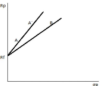
Figure 8. The efficient portfolio. (Made by the authors of this paper and based Elton et al., 2007)

In Figure 8, seen above, two different portfolios are drawn. One can clearly see that fund B gives a higher return than fund A, however, noting that the first mutual fund has a higher Sharpe ratio indicated by the steeper line. Assuming that the investor can

bor-21

row and lend for the same risk-free rate, he or she can borrow and invest in mutual fund A and thus move it to A´, making it possible for the investor to gain the same return for his investment as in mutual fund B although given a lower risk. By applying the under-standing of borrowing and lending for the same risk-free rate, the investor can achieve superior returns, thus making clear that the higher Sharpe ratio would always be the best choice.

2.7.2 O ther T echniques of risk-adjusted performance

Although the Sharpe Ratio is the most common ratio when measuring the risk-adjusted performance, there are other recognized measures, such as Jensen, Treynor and Modi-gliani-Modigliani. The Modigliani measures risk-adjusted performance by measuring the return adjusted to the risk, and comparing it with a benchmark of some kind e.g.

market portfolio or index portfolio (Modigliani and Modigliani, 1997). A simple

expla-nation could be that, the Mogliani measure says what return the mutual fund or portfolio would have, given it had the same risk as the market index (Simons, 1998).

Both Jensen and Treynor use the systematic risk when measuring for the risk-adjusted performance (Elton et al., 2007). The systematic risk would be especially important when measuring the performance of a mutual fund that is part of a portfolio. This due to them being diversified well enough to leave only a market risk that needs to be adjusted for (Simons, 1998).

22

3

Method

This chapter of the thesis will give the reader an understanding of the methods used for the empirical results. The reader should understand this section in order to better grasp the results of this paper.

3.1

Regression Analysis

To achieve our purpose, to test if the excess returns of Swedish equity mutual funds can be explained by the fund’s portfolio turnover rate, a linear regression analysis was per-formed.

A linear regression is a method to test the relationship between a dependent variable and a set of independent variables. In a simple regression, a regression with only one inde-pendent variable, the analysis indicates how a change in the indeinde-pendent variable affects the dependent variable when the dependent variable is held constant. Using a linear re-gression, equation (5), we tested if our dependent variable, the excess return, can be ex-plained by the independent variable, the portfolio turnover rate.

(5)

In general, regression models such as equation (5) rely on four key assumptions; 1. Linear relationship between the dependent and independent variable 2. Independence of errors

3. Homoscedasticity (Constant variance) of errors a) Residuals versus time

b) Residuals versus independent variable 4. Normality of error distribution

A violations of the above assumptions, in particular the first assumption, indicates no relation between the variables. Further, the interpretation of the results produced by the regression model might be inefficient or biased. In our sample, assumption 2 and 3a are not relevant since they require a time series data. For that reason, we do not consider

23

them. As for the normality of the error distribution, we assume the Central Limit Theo-rem (Gujarati, 2003).

However, as such regression might be exposed to omitted variables bias, incorrectly leaving out important factors of the model, we added control variables as shown in

equation (6). We added the following variables to test the relationship between the PTR

and excess return; Management fee, Age, and Size.

(6)

3.1.1 Excess Return

The excess returns, achieved in accordance with Gruber (1996), were calculated by

equation (2). The calculations are based on a time period of 60 months, from

2007-01-01 to 22007-01-011-12-31. To be able to perform a consistent regression, the first step was to transform the monthly returns of each fund and the monthly market returns into yearly returns. This was done to match the yearly calculation of the PTR.

The sample data for the returns of each fund was received from Morningstar and were transformed by adding the returns from January to December of each year and then di-vide each year by 12. In other words, the average of each year’s return for each fund was used as the yearly return. For the market return, we chose to use the index over the 30 largest traded stocks on the Stockholm Stock Exchange, OMXS30. The closing pric-es for OMXS30 were obtained from Yahoo Finance and transformed into monthly mar-ket returns by equation (7).

(

) (7)

In equation 7, the market return, Rm,t, was calculated by taking the natural log of the

first months closing price, (CPt), divided by the closing price of previous month, (CPt-1).

aver-24

age. The excess return used in the regressions were calculated for each year for every fund by equation (8).

(8)

Repeating equation (8) for all five years and dividing by five, gave us the average ex-cess return that were used in the regressions, see appendix 2.

3.1.2 Portfolio T urnover Rate

The independent variable, PTR, was collected from each funds factsheet and annual re-port for all five years. Having the PTR of each fund between the years 2007-2011, an average was taken to be comparable to the excess returns.

3.1.3 Management fee

Liljeblom and Löflund (2000) found that fund expenses such as management fee are significantly related to fund performance. Hence, our first control variable in the regres-sion is the management fee of all funds. The variable is in percentage terms the fee which is charged by the funds, furthermore, it is a percentage of the total value of the fund. Although received from Morningstar as an percentage value, we will consider it as an ordinary number in the regressions. Hence, a management fee of 1 percent which normally would be 0.01, will in the regression be considered as 1. Further, in line the study by Berk and Green (2002), we will assume that management fee does not change during our time period.

3.1.4 Age

In a study by Bams and Otten (2002), the age was found to have a negative effect on the performance. We calculated the age by using the inception day, received from Morn-ingstar, and counted the months between the inception day and the last month of 2011. Similar to the assumption made for the management fee, we will assume that the age of the funds is fixed and does not vary during our time period. In other words, we will as-sume the age to be the same in 2007 as in 2011

25 3.1.5 Size

Grinblatt and Titman (1989) found that size of mutual funds had an effect on the per-formance, as a result, the last control variable in our regression is the size. We measured the size of each fund by the total value of the funds. The total value was gathered from the Swedish Financial Supervisory Authority’s webpage (finansinspektionen.se) and was calculated by taking the average of the five years.

3.2

Linearity T est

Non-linearity is usually most evident by plotting the variables. Hence, the first step in analyzing the regression model of equation (5) was to plot the data for our two variables in a scatterplot. An alternative approach, using the regression output, was also per-formed. Here, the residuals are plotted against the predicted values. The points from this approach should be along or around a diagonal a line in a systematic distribution. In a case where the relationship between the dependent and independent variable are non-linear, a transformation of the variables might solve the non-linearity (Gujarati, 2003). We applied three non-linear transformations to test whether it would have any effects. The transformations we carried out where:

i. A log transformation of the portfolio turnover rate.

(9)

ii. An additional regressor was added; the portfolio turnover rate squared = PTR2. (10)

iii. An exponential transformation of the Sharpe ratio.

(11)

3.3

H omoscedasticity T est

b) Testing residuals versus the predictions and independent variable.

This assumption, related to the alternative approach above, indicates that the variation of the residuals from the regression line in the regression output should be the same for

26

all values of the independent variable. In other words, the variance for the residuals around the regression line should be the same no matter if the PTR values are high or low. To be thorough, we also plotted the residuals against the independent variable to see if the residuals are randomly distributed. This means that there should be no pattern of the residuals. Most often, heteroscedasticity is a result of a significant violation of the linearity assumptions, hence, it can be fixed as by fixing through the non-linear trans-formations above (Gujarati, 2003).

3.4

Further Assumptions

The funds in our study are based on Morningstar’s definition of Swedish equity mutual funds investing in Sweden. In our sample, we have removed all funds where the base currency is of foreign nature and those which the PTR could not be found. Since we considered funds from 2007-01-01 to 2011-12-31, all funds with an inception day after 2007-01-01 are removed from the sample. Further, we only study funds that that have survived until the end of the sample period. Hence, our sample selection suffers from survivorship bias. According to Carpenter and Lynch (1999), survivorship bias is a phe-nomenon where only funds that have survived until the end of the sample period are in-cluded. This is common in the fund industry and result in mutual funds overestimating their performance (Elton et al., 2006). The risk-free rate, a 10 year Swedish government bond, was gathered from the Swedish federal bank (Riksbanken) for each of the five years. The choice of risk-free rate is based on Damodaran’s paper “What is the riskfree

27

4

Empirical findings

This part of the thesis will give the reader of this paper a good overview of the statisti-cal results. The authors will try to give the readers an overall view of the statistics that will hopefully give the reader a solid ground to stand on, before getting to the analysis.

4.1

Summary of Descriptive Statistics

Table 4-1 shows the descriptive statistics found for the sample. The number of

observa-tion for all the tests is N=45. There is a reasonably large difference in the activity of the funds in the sample. The minimum PTR is 0.12 times per year and the maximum is 4.98 times per year. When then looking at the minimum and maximum for the excess return we can see a maximum return of 0.533 and a minimum return of -0.082. With this ob-servation in mind we can see that there is a large difference in the minimum and maxi-mum of excess returns and PTR. We can also see that the standard deviation for PTR is larger than the standard deviation of the excess return. The difference of mean and me-dian values for excess return is minor while we can see a relatively large difference for these values for the PTR. Hence, the most reasonable interpretation is that the excess re-turn is not explained by the PTR.

Table 4-1. Descriptive Statistics

PTR Excess return Median 0.524 0.178 Mean 0.82 0.160 Max 4.98 0.533 Min 0.12 -0.082 Std.Dev. 0.859 0.142 N 45 45

4.2

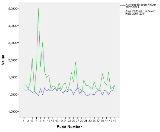
Graphing the relationship

In figure 9 the relation between the Portfolio Turnover Rate (green line in figure 9 ) and the excess return (blue line in figure 9 ) is illustrated. A relatively consistent pattern can be observed in the average excess return compared to the high variation in the Portfolio Turnover Rate. It is difficult not staring at the PTR for Fund number 9, as even with a

28

PTR of 4.98, the excess return remains in line with the overall mean. We can however notice some patterns between the two lines; for the overall sample we can see a hint of negative relationship for the two variables when moving at opposite directions, howev-er, in between case number 15 to19 there seems to be a positive correlation in the two variables.

Figure 9.Graph presenting excess return and PTR

The overall poor performance of the funds is due to the weak economic climate in year 2008 and 2011. Although the funds have experienced positive returns in-between the fi-nancial crises, the bad years outweighed the positive years.

4.3

O utput of regression models

Figure 9, in section 4.2, was a first graphical observation on the relationship between

29 Table 4-2. Regression on equation (4)

Variable B P-value

Constant 0.203 0.000***

PTR -0.052 0.037**

R-square 0.097

N 45

Notes: The variables are statistical significant when α > P-value;*** significant on the 1% level. ** significant on the 5% level and * significant on the 10% level.

The slightly negative coefficient of the PTR in table 4-2, indicates that a fund which is more active would have a negative impact on the excess return. In contrast, a less active fund would have a positive effect on the excess returns. At a significance level of five percent, this holds true, while at the one percent significance level this is rejected and no relationship is supported. The constant variable is statistically significant on all three significance levels. However, as the constant term gives the predicted value of the de-pendent variable when the predictor is set to zero, it does not give any economical inter-pretation. Further, the R-square term indicates that the model where the PTR is predict-ing the excess return is poorly suited. As a result, one has to be careful with the eco-nomic interpretation from the regression.

Including the control variables to equation (5) and performing a linear regression on

equation (6), presented a noteworthy outcome. While the PTR is still marginally

nega-tive in table 4-3, testing the statistical significance on one, five, and ten percent, indi-cates that the PTR does not influence the excess return. Performing the same tests on the control variables indicates that neither one has any statistical effect on the excess re-turn. Although the R-square is twice as high as the first regression, it is still a poorly de-scriptive measure. Further, the low value of adjusted R-square indicates that when more independent variables are included, the amount which they explain the excess return re-duces. In other worlds, their predictive power decrease, which most likely is a result of multicollinearity.

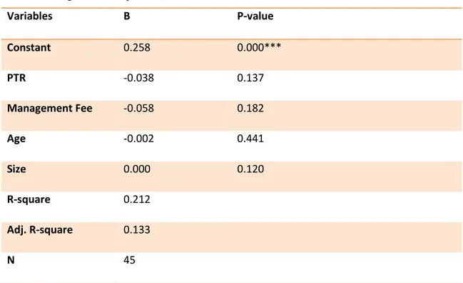
30 Table 4-3. Regression on equation (6)

Variables B P-value Constant 0.258 0.000*** PTR -0.038 0.137 Management Fee -0.058 0.182 Age -0.002 0.441 Size 0.000 0.120 R-square 0.212 Adj. R-square 0.133 N 45

Notes: The variables are statistical significant when α > P-value;*** significant on the 1% level. ** significant on the 5% level and * significant on the 10% level.

4.3.1 Yearly Regressions

Replicating equations (5) and (6) for each year, as shown in appendix 2, is performed to see if the outputs in section 4.3 is caused by one particular period. Evident from the outputs is that the PTR, both for equation (5) and (6), is statistically insignificant for all years. Further, the control variables are all found to be statistically insignificant for all years except 2008 when the management fee is found to be statistically significant on the ten percent level and the age on the five percent. However, consistently for all re-gressions is the low prediction power of the models, as shown by the low R-square.

4.4

Linearity T est

The dots in figure 10 should be along or around a diagonal a line in a systematic distri-bution. As is evident from the figure, there is no systematic distribution of the dots. This is in line with the conclusion drawn in section 4.3 that there is no relationship between the dependent and independent variables.

31 Figure 10. Linearity Test

4.5

H omoscedasticity T est

Building on the same conclusions as in section 4.3 and 4.4, the homoscedasticity test indicates once again that there exist no relationship between the dependent and inde-pendent variables. The residuals exhibit different variability around the regression line. Put differently, the variance for the residuals around the regression line is not the same when the value of PTR changes.

32 Figure 11. Homoscedasticity Test

33

5

Analysis

The goal with active management is to achieve superior returns with the help of fore-casting methods. Managers generally use either fundamental analysis or technical anal-ysis before making their decision. The definition of active management demands that the active portfolio takes positions that are different from that of a passive portfolio or comparable passive benchmark (Elton et al., 2007). Our aim with this thesis was to see how and if the degree of a portfolios activity could explain the excess return of mutual funds. A similar study was presented by Chen et al., (2000), on whether funds that trade more actively have better stock-picking skills than other funds, and thus reach higher re-turns.

When observing the descriptive statistics, we can see that the dispersion from the mean for the PTR and excess return in our sample exposed a relatively high standard devia-tion of 0.859 for PTR, in comparison to the standard deviadevia-tion of 0.143 for excess re-turn. Hence, the high variation in PTR does not affect the excess rere-turn. As indicated by the low variation of the excess return, even if a higher PTR would result in higher excess return and low PTR would result in a low excess return, the difference would be minimal. This suggest that they have not been successful in their active management, and the empirical results obtained are consistent with the theory of market efficiency. This does on the other hand not exclude that active management might find anomalies in the market, in which some, like Dimson and Massoud (1998) call “merely statistical oddness”. According to Dimson and Massoud anomalies do not imply a rejection of the efficient market hypothesis as they are simply still called “anomalies”. Most scholars argue that anomalies occur in most markets, however managing to exploit these before they close is much more difficult.

Further, the regression output in table 4-2, indicates a negative relationship between excess return and PTR on the five and ten percent significance level, while it is insignif-icant at the one percent significance level. Hence, the results indicates that a less active fund would have a positive effect on the excess returns. This matches the findings made by Elton et al. (2006), which also found that funds with a low activity have higher per-formance. Noteworthy is that when the age, size and the management fee was added to the regression, the PTR did not show any effect of the excess returns. Using the

con-34

cepts of Gujarati (2003), this is most likely a result of the low value of the adjusted R-square and the relationship between the predictors. Hence, adding the control variables made the PTR lose predictive power of the excess returns and resulted in no signifi-cance of the relationship. Further, this indicates that the first regression is most likely subjected to omitted variable bias. Ippolito (1993), presents arguments similar to those find in our thesis. The overall low R-square from the regression outputs indicates how poorly the a regression line estimates the real data. Hence, one has to be careful with the economic interpretation. Further, the relationship between the PTR and excess return could not be traced to a particular year.

Our study suggests that the mutual fund managers might have failed in grasping the gaps in the market that are not commonly known (with “commonly known”, we refer to

theories such as the January effect and the day-to-day effect). Our results can however

not exclude that patterns such as The Incredible January Effect by Haugen and Lakonishok may exist in the Swedish market, it may however be likely that known gaps have been closed as soon as the articles of these theories were published.

The main difference between our findings and previous research, is the time period. One could argue that the period from which we measured data was during a quite intense re-cession, and although this might not be the sole factor, one needs to be critical to this el-ement. The time period we have chosen to test for is exceptionally unusual, as we are witnessing a extreme financial crises. The recession started in the year 2008 and is con-tinuing to this day. It has affected the global economy as a whole and financial institu-tions have fallen. The financial market has not remained outside the great impact caused in this period. One needs to remember that mutual funds that have a high PTR might be subjected to high costs for the information they obtain, and consequently fees may arise for the investor. The investor needs in this case be certain that there is an extra return gained from the active management that will cover the fees.

35

6

Conclusion

As the mutual fund market has grown to be a favorable investment technique of Swe-dish investors, the need for an appropriate way to evaluate the funds has never been as valuable. In a more active mutual fund, the fees associated with the investment are more likely to be higher. Hence, the most reasonable interpretation would be that the fees are justified with higher return. However, when weighing the evidence found in the under-lying thesis, it appears more likely that investors should avoid funds with more active nature.

Using the portfolio turnover rate (PTR) as a measure of activity the purpose of this the-sis is to test whether the excess returns of Swedish equity funds could be explained by the PTR between the years 2007 to 2011. From a simple regression, using PTR as inde-pendent and excess returns as deinde-pendent, a negative relationship between the variables was found. Although this is in contrast to the findings by Dahlquist et al. (2000), they are in line by those of Elton et al. (2006). On the other hand, the regression violated two of the four key assumption; first, linear relationship between the dependent and inde-pendent variable and second, constant variance of errors. Hence, the results are most likely to be inefficient. This is also evident from the extremely low R-square value. Furthermore, when adding management fee, size and age to avoid the omitted variable bias, no relationship was found between the PTR and the excess return, similarly argued by Ippolito (1993).

The time-period in the study is a extraordinarily one, the financial turmoil during this period have aggravated the returns of the funds. In an attempt to diminish the effect of the financial crises, yearly regressions was performed to see if there existed any rela-tionship between excess return and PTR. The same method was performed for the con-trol variables. However, this study found no evidence of any relationship between ex-cess return and PTR, with or without any control variables.

A recommendation for future research would be to investigate the activity of funds dur-ing different economic conditions. This would be of assistance to determine if the activ-ity of funds is dependent on the economic environment.

36

List of references

Articles

Bams, D. and Otten, R. (2002). European Mutual Fund Performance, European

Finan-cial Management, Vol 8.(1), pp.75-101

Belvers. R.J. (1990). Predicting Stock Returns in an Efficient Market. The Journal of

Finance. Vol. 45(4). pp. 1109-1128.

Berghuis. W.H. (1967). Onstaan en Ontwikkeling van de Nederlandse Beleggingsfond-sen tot 1914. dissertation Van Gorcum & Comp.. AsBeleggingsfond-sen.

Berk, J. B., and Green, R. C. (2002). Mutual Fund Flows and Performance in Rational Markets, Working Paper 9275, National Bureau of Economic Research

Bushee B.J. and Abarbanell J.S. (1997). Fundamental Analysis. Future Earnings. and Stock Prices. Journal of Accounting Research. Vol. 35(1). pp. 1-24.

Carhart. M. (1997). On Persistence in Mutual Fund Performance. The Journal of Fi-nance. pp 67-82.

Carpenter. J. N. and Lynch. A. W. (1999). Survivorship bias and attrition effects in measures of performance persistence. Journal of Financial Economics 54. pp. 337-374 Chen. H.. Jegdeesh. N. and Wermers. R. (2000). The value of Mutual Fund Manage-ment: An Examination of the Stockholdings and Trades of Fund Managers. The Journal

of Financial And Quantitative Analysis. pp 343-368.

Dahlquist. M.. Engström. S. and Söderlind P. (2000). Performance and Characteristics of Swedish Mutual Funds. University of Washington School of Business Administration. pp 409-423.

Damodaran. A. (2008). What is the risk-free rate? A Search for the Basic Building Block. Stern School of Business. New York University

Dimson. E. and Massoud. M. (1998). A Brief History of Market Efficiency. European

Financial Management. Vol. 4(1). pp. 91-193.

Fama. E. and French. K. (1988). Permanent and Temporary Components of Stock Pric-es. Journal of Political Economy. Vol. 96(2). pp. 246-273.

Fama. E.F. (1965). The Behavior of Stock-Market Prices. The Journal of Business. Vol. 38(1). pp. 34-105.

37

Fama. E.F. (1970). Efficient Capital Markets: A Review of Theory and Empirical Work.

The Journal of Finance. Vol. 25(2). pp. 383-417.

Frennberg. P. and Hansson. B. (1993). Testing the random walk hypothesis on Swedish stock prices: 1919-1990. Journal of Banking & Finance. Vol 17. pp 175-191.

Grinblatt. M. and Titman. S. (1989). Mutual Fund Performance: An Analysis of Quar-terly Portfolio Holdings. The Journal of Business. pp 393-416.

Grossman. S. J. and Stiglitz. J. E. (1980). On the Impossibility of Informationally Effi-cient Markets. The American Economic Review. Vol. 70(3). pp. 393-408.

Gruber, M. J. (1996). Another Puzzle: The Growth in Actively Managed Mutual Funds.

The Journal of Finance, vol. 51(3). pp. 783-810

Ikenberry. D.. Shockley. R. and Womack. K. (1998). Why active fund managers under-perform the S&P 500: The impact of size and skewness. The Journal of Wealth

Man-agement. pp. 13-26.

Ippolito. R. A. (1993). On Studies of Mutual Fund Performance. 1962-1991. Financial

Analysts Journal. Vol. 49(1). pp. 42-50.

Jensen. M. C. (1967). The Performance of Mutual Funds in the Period 1945-1964.

Journal of Finance. Vol. 23(2). pp. 389-416.

Levy. H. and Sarnat. M. (1970). International Diversification of Investment Portfolio.

The American Economic Review. Vol. 60. No. 4. pp. 668-675

Liljeblom, E. and Löflund, A. (2000). Evaluating mutual funds on a small market: is benchmark selection crucial? Scandinavian Journal of Management, Vol. 16, pp. 67-84. Malkiel. B.G. (2003). The Efficient Market and Its Critics. The Journal of Economic

Perspectives. Vol. 17(1). pp. 59-82.

Markowitz. H. M. (1952). Portfolio selection. The Journal of Finance 7. 77-91.

Markowitz. H. M. (1991). Foundations of Portfolio Theory. The Journal of Finance. Vol. 46(2). pp. 469-477.

Mazuy. K. and Treynor. J. (1966). Can Mutual Funds Outguess the Market?. Harvard

Business Review. pp 131-13.6.

Modigliani. F. and Modigliani. L. (1997). Risk-Adjusted Performance: How to Measure it and Why. Journal Of Portfolio Management. Vol. 23. pp. 45-54.

38

Rouwenhorst. K.G. (2004). The Origins of Mutual Funds. Yale International Center for

Finance Working Paper. No. 04-48. pp. 1.

Schreiner. J. (1980). Portfolio Revision: A Turnover-Constrained Approach. Financial

Management Association International. Vol. 9(1). pp.65-75

Sharpe. W. F. (1993). International Value and Growth Stock Returns. Financial

Ana-lysts Journal. Vol. 49(1). pp. 27-36

Simon. E.W. (2002). Anomalies and Market Efficiency. Working Paper.. The Bradley

policy Research Center. No. 02-13. University of Rochester

Simons. K. (1998). Risk-Adjusted Performance of Mutual Funds. New England

Eco-nomic Review. Sep/Oct. pp. 33-48.

Miller. K. and Samak. V. Sorensen. E. (1998). Allocating between active and passive management. Financial Analysts Journal. pp 18-31.

Tobin. J. (1958). Liquidity Preference as Behavior Towards Risk. The Review of

Eco-nomic Studies. Vol. 25(2). pp. 65-86.

Ziemba. W.T. and Hensel C.R. (1994). Worldwide Market Anomalies. The Royal

Socie-ty Stable. Vol. 347(1684). pp. 495-509.

Books

Damodaran. A. (2002). Investment Valuation; Tools and Techniques for Determining

the Value of Any Asset (2nd ed.). John Wiley & Sons: New York.

Elton. E. J.. Gruber. M. J.. Brown. S. J. and Goetzmann. W. N. (2007). Modern

Portfo-lio Theory and Investment Analysis (7th ed.). John Wiley & Sons: New York.

Gujarati. D. N. (2003). Basic Econometrics (4th ed.). Singapore: McGraw-Hill Educa-tion.

Markowitz. H. M. (1959). Portfolio Selection: Efficient Diversification of Investments.

New York: John Wiley & Sons.

Electronic sources

The Swedish Investment Fund Association. (2009). 30 år med Fonder. Retrieved from

http://www.fondbolagen.se/upload/30_ar_studie.pdf on March 7. 2012.

Swedish Investment Fund Association. Retrieved from

39

Swedish federal bank (Riksbanken), Retrieved from

http://www.riksbank.se/sv/Rantor-och-valutakurser/Sok-rantor-och-valutakurser/?g7-SEGVB10YC=on&from=2006-12-31&to=2011-12

40

Appendix 1

Yearly Excess Return Calculation

For 2007: For 2008: For 2009: For 2010: For 2011: Average 2007-2011: ∑