Develop Optimization Model for Spheroidal Graphite Iron

(1)

Develop Optimization Model

for Spheroidal Graphite Iron

AUTHOR: Rehman Babar

SUPERVISORS: David Samvin and Johan Jansson

JÖNKÖPING

(2)

Preface

This thesis work has been carried out at the School of Engineering in Jönköping in the department of Industrial Product development, Production and Design. The work is a part of the two-year Master’s program in Product Development and Materials Engineering.

The authors take full responsibility for opinions, conclusions and findings presented.

Examiner: Kent Salomonsson

Supervisor: David Samvin and Johan Jansson Scope: 30 credits

(3)

Acknowledgments

I express my sincere gratitude to my supervisorSenior Lecturer David Samvin and Doctoral student Johan Jansson, Jönköping University for their valuable suggestions, motivation, and excellent guidance during this thesis work.

I would like to thank all my friends who supported me in my studies. most importantly Mr. Rishab Karan Mehta.

At the last, not least, I would like to thank my parents and my family who supported me and for their endless love.

Sincerely, Rehman Babar

(4)

Abstract

The main motivation behind this study is to develop a methodology to generate surrogate model coefficients for parametrized Spheroidal Graphite Iron (SGI) for thermal expansion and Young’s modulus response. To accomplish this objective, a 3D model was created by Abaqus, and Python was used for developing the script. The design of experiments (DoE) was utilized to compute two objectives parametrically. The inputs in this thesis were Poisson’s ratio, Young's modulus, radius, and volume fraction of Graphite, Ferrite, and Pearlite. Then DoE is integrated with Abaqus to get homogenized properties of the SGI in terms of Coefficient of thermal expansion (CTE) and Young’s modulus. Using these homogenized properties, the surrogate model coefficients were obtained, and Young’s modulus-CTE graph was visualized.

(5)

List of Figures:

Figure 1: Illustrates the microstructure of ductile cast iron [17] ... 12

Figure 2: Ferritic ductile iron microstructure [1] ... 13

Figure 3: Pearlitic ductile iron microstructure [1] ... 13

Figure 4: Austempered ductile iron microstructure [1] ... 14

Figure 5: Demonstrate silicon content to carbon content percentages [6] ... 15

Figure 6: Strain-strain diagram [9] ... 17

Figure 7: Showing the cube for BBD design [12] ... 19

Figure 8: Shows Pareto Optimal solution, Parameter space and Function space [15] ... 21

Figure 9: Flowchart shows complete methodology and implementation of this project ... 22

Figure 10: Shows the Sectional representation of Graphite, Ferrite, Pearlite ... 23

Figure 11: Three sections with different materials ... 23

Figure 12: Abaqus 3D model code as function ... 24

Figure 13: Obtaining input values by sys.argv ... 27

(8)

List of Tables:

Table 1: The average composition of SGI [17] ... 16

Table 2: Input values ... 27

Table 3: Detail information about the Abaqus output file ... 30

Table 4: The Box Behnken DoE layout ... 31

Table 5: The Box Behnken DoE with input values ... 31

Table 6: The homogenized average values of Young's modulus and CTE ... 32

Table 7: Combine DoE with output values... 33

(9)

1. INTRODUCTION

Ductile cast iron or SGI – Spheroidal Graphite Iron is a very commonly used alloy in industry due to its vast applications since its microstructure can be controlled by varying temperatures e.g. the cooling rate hence many possible structures can be generated which creates a range of possible iron alloys with different physical properties. This project will focus on studying the microstructure of SGI and developing a tool which uses Abaqus and also optimizes SGI’s properties. Many parameters will be integrated and DoE- design of experiments will be generated to study the optimal solution from all experiments. These experiments will be performed in Abaqus.

The term cast iron implies to an alloy of iron containing more than 2% carbon. The brittle behavior related to cast iron is an obsolete and generally misguided judgment which infers all cast irons are fragile and none of them are ductile. Ductile iron is one type of cast iron that is ductile and it offers the designer a remarkable mix of high strength, wear resistance, fatigue resistance, toughness, and pliability in addition to great castability, machinability, and damping properties. These characteristics of SGI are not considering the misinterpretation of its fragile nature. SGI having a carbon content of over 3% and graphite present in spherical shapes [1]. As the percentage of carbon increase iron getting soften and heat transfer increase as well but addition of magnesium will increase the hardness.

1.1 Background

SGI was found in 1948 at the American Foundrymen Society Annual Conference, which is a kind of graphite-rich cast iron. When magnesium was added, the graphite formed nodules instead of flasks. While most alloys of cast iron are weak in tension and because of its nodular graphite considerations, brittle and ductile iron have significantly more effect on fatigue resistance. On October 25, 1949, Keith Millis, Gagnebin, and Norman Pilling got a US patent no. 2485760 on a Cast Ferrous alloy for ductile iron formation by strategies for magnesium treatment. Augustus F. Meehan was allowed a patent in January 1931 for inoculate iron with calcium silicide to make ductile iron likewise Known as Meehanite, which was delivered in 2017 [2] [3].

In nature, iron is present in the form of an ore, which is stone in physical appearance and contains lots of impurities. By melting iron ore, pig iron is obtained which is the rawest form of iron ore. By melting pig iron and removing impurities Cast iron is obtained which still has other elements like carbon and silicon. Cast iron is an alloy which has iron with more than two percent carbon, the ratio of carbon changes the physical and thermal properties of the alloy, thus, there are many possible states in cast iron. Due to the lower melting points and castability,

(10)

iron carbide is formed, while if the percentage of silicon is high then carbon is removed from the solution and graphite is formed which is called grey cast iron. There are many other alloying elements, for example, Mn, Mo, Ti, etc. The ratio of these alloying elements forms a different form of structure and make different types of cast iron.

Gray cast iron and white cast iron are two main classifications of the cast iron. Gray cast iron has a gray fracture appearance while white cast iron has a white fracture appearance. these names apply today while, other cast irons have been developed which have their name derived from their mechanical property, as ductile iron and malleable. The type of cast iron depends on four main factors which are, the content of carbon, the content of impurity, the alloy, the heat treatment, and the cooling rate. These boundaries control the structure composition and the form of the matrix phase [1][2].

(11)

1.2 Purpose and Goals 1.2.1 Purpose

This thesis focuses on developing a script to obtain an optimized model for SGI cast iron. For an optimized model is it necessary to compute the surrogate model coefficient beta, which can be obtained by design of experiments approach. The design of experiment is used to compute the two objectives Young’s modulus and coefficient of thermal expansion parametrically. The input parameters used for this parametric study are Poisson’s ratio, Young’s modulus, radius and volume factions of Graphite, Ferrite and Pearlite.

1.2.2 Goals

➢ Develop a script that will generate a surrogate model of DoE results from the 3D Finite Element model of SGI.

➢ Develop a script to apply optimization algorithms to the surrogate model. ➢ Develop a script to visualize the Pareto optimal solutions.

(12)

1.3 Delimitations

There are four main delimitations are applied in this thesis which are:

• The values selected for developing scripts are chosen randomly since the thesis is based on developing the script rather than computing a finite element problem.

• To reduce the computation time 10 inputs related to volumes fraction were considered out of 22 inputs, 12 of which are thermal parameters.

• There is a total of 66 surrogate model coefficients but only 21 coefficients were considered since the remaining do not affect the accuracy of the solution.

• The values used for the Representative Volume Element (RVE) in the thesis are not real values but rather than artificial and highly simplified RVE, to demonstrate the methodology.

(13)

1.4 OUTLINE

Background of

SGI

• Types of SGI

• Properties and Composition of SGI • Young's modulus and CTE

• DoE

• Box-Behnken Design

• Surface response & Pareto Analysis and Surrogate Modeling

Method and

Implementations

• Abaqus Model

• Python Implementation • Making DoE from Inputs • Connecting DoE with Abaqus • Compiling results and plotting

Results

• Abaqus Results

• Creating Box Behnken Layout and Replacing Inputs • Computing out values

• Combine DoE with output

• Plotting Young's modulus and CTE

(14)

2. THEORETICAL BACKGROUND

2.1 Ductile Cast Iron – SGI

SGI cast iron is produced by following special alloy addition and proper cooling speeds so that the carbon can be converted into spherical forms and will be used in those fields where carbon in flake or temper form can't be utilized. During the solidification, nodules will be formed while in heat treatment nodules are not formed but will change mechanical properties. It can be of three types pearlitic, ferritic, and martensitic, and has better mechanical properties that can compare with steel. There is a subclass of ductile iron that has the same spherical graphite and nodular as ductile iron while the matrix is a combination of stabilized austenite and bainite. That subclass of ductile iron is known as Austempered ductile iron. So Austempering is required for this kind of cast iron structure [2][4]. The shape of graphite is controlled by small alloying addition as shown in figure 1.

Figure 1: Illustrates the microstructure of ductile cast iron [17]

2.2 Types of SGI

SGI can be classified into four groups base on matrix phases. 1. Ferritic

2. Pearlitic 3. Martensitic 4. Austenitic

SGI is generally ferritic type, but it is difficult to be used in a particular application because of high ductility and low yield strength. Consequently, if some carbon is left deliberately in the cementite form, property gets enhanced. Such type of SGI is referred to as pearlitic SGI. If

(15)

the cooling rate is very high martensite will produce from the matrix. The applications of SGI are limited due to ductility. so, the matrix may fluctuate from a hard-pearlitic structure through a soft ductile ferritic structure [5].

Figure 2: Ferritic ductile iron microstructure [1]

(16)

Figure 4: Austempered ductile iron microstructure [1]

Carbon and Iron at different temperatures and different percentages of ratio create different structures as shown in the following figure 5. It shows that there are three main regions which are separated by two lines where carbon is at 0.16 and Si percentage is 2 which separates Steels and malleable cast iron, which means below this line it will be called steel while with a percentage higher than 2% will form malleable cast iron, similarly before carbon and 0.33 Si percentage lesser than 4.3 as shown will be malleable while more than that will form ductile cast iron also known as SGI [6].

(17)

Figure 5: Demonstrate silicon content to carbon content percentages [6]

2.3 Properties and Composition of SGI

The mechanical properties, physical properties, and service properties were taken into consideration while selecting any material to be used for industrial applications. The mechanical properties like rigidity, hardness, elastic modulus, tensile strength, and yield strength and physical properties include damping limit, machinability, and conductivity are taken into consideration. The material to be utilized ought to have survived under service conditions and it can be measured by heat resistance, wear resistance, and corrosion resistance. Properties:

Tensile Strength: The tensile strength is the maximum longitudinal stress that a material withstands before its fracture. The tensile strength in ductile iron from 414 MPa for ferritic grades to more than 1380 MPa for martensitic grades.

Yield Strength: The yield strength is the amount of stress at which a material starts to plastically deform. The yield strength ranges from 275 MPa for ferritic grades to 620 MPa for martensitic grades.

(18)

Modulus of Elasticity: Ductile irons show a relative stress-strain limit which seems to be like that of steels yet is hampered by plastic deformation. The modulus of elasticity varies from 162-170 GPa.

Excellent Corrosion Resistance: Ductile irons have very the best corrosion resistance property.

Machinability Has generally excellent machinability due to the graphite which is accessible in free form. So, chip development is easier.

Cost-Strength Ratio: The cost per unit strength value is lower than most of the materials. In this manner, it has a wide scope of uses for which it tends to be utilized [7].

And the table shown below describes the average composition of SGI. Table 1: The average composition of SGI [17]

Element

Content (W.R.T %)

Carbon

3.2 – 3.6

Silicon

1.8 – 2.8

Manganese

0.03 – 0.04

Phosphorus

0.005 – 0.04

Sulphur

0.005 – 0.02

2.4 Young’s modulus

In structural engineering of Cast iron, the main purpose is to optimize structural properties which mainly include modulus of elasticity. Young’s modulus is called modulus of elasticity (E) is the most important property of solids, that describes material stiffness. The stress-strain curves explained how material store energy in form of stress and its stiffness. The strain is defined as a change in length per unit original length and stress is defined as a force per unit area [8]. The degree of formation depends on the material size. The stress and strain can be presented by Hooke´s Law (stress is directly proportional to strain):

From Hook’s law the modulus of elasticity is defined as the ratio of the stress to the strain:

(19)

where σ

is stress, E is Young’s modulus, and

ε

is a strain. Graphically we can define modulus of elasticity as a slope of the linear portion of the stress-strain diagram as follows.

Figure 6: Strain-strain diagram [9]

2.5 Coefficient of Thermal Expansion

The coefficient of thermal expansion (CTE) defines the geometrical changes in the structure due to temperature change, it functions due to the change of microstructure. In SGI Coefficient of thermal expansion has specific significance since it is an alloy where graphite is embedded in a continuous matrix [10].

The thermal expansion produce change in the volume of material thus material expands as result. Relative expansion in the case of thermal expansion is also called a strain, the ratio of this strain with a change of temperature is defined as the material’s coefficient of thermal expansion.

There are three types of CTE mentioned as following: • Linear coefficient of thermal expansion

• Area coefficient of thermal expansion • Volumetric coefficient of thermal expansion

The volumetric coefficient of thermal expansion for general for gas, liquid, or solid-state is mentioned as following [10]: α = αV= 1 V( ∂V ∂T)p (2)

(20)

2.6 DoE – Design of Experiments

Design of experiments is a very common step in multiparametric optimization, in multiparametric optimization, there are many input parameters and output parameters, every input parameter generally changes output, thus many input and out parameters are related to each other, all output solutions are attached to input parameters. Input parameters boundary conditions are determined normally found from research or previous experience to check where it can work and where cannot work, after finding the possible region, the input parameters boundary conditions are correlated with the output parameters and experiments are created, the number of experiments is normally dependent on the number of input parameters if input parameters are large in number to find the correlation between each parameter with others to find a desired Multiobjective solution will require a high number of experiments. Thus, the design of experiments is the most important phase in multiparametric optimization [11].

This thesis aims to develop a methodology to generate surrogate model coefficients for parameterized SGI, which has many physical inputs parameters mentioned as following:

• Young’s modulus • Poisson ratio • Volumetric ratio • Ferrite thickness • Graphite Radius 2.7 Box Behnken Designs

Box-Behnken designs (BBD) are a class of rotatable or nearly rotatable second-order designs based on three-level incomplete factorial designs [11]. It is an exceptional 3-level plan since it does not contain any focuses at the vertices of the examination district. This could be favorable when the focuses on the edges of the 3D square speak to level blends that are restrictively costly or difficult to test due to physical cycle limitations. For three factors its graphical portrayal can be found in the structure. All the center points and the middle points in a cube at which Box Behnken design concentrates can be seen in figure 7. In Box Behnken designs each factor is an independent variable that is placed at three values in space as mentioned as +1, -1, and 0.

(21)

Figure 7: Showing the cube for BBD design [12]

For Box Behnken, the number of the experiment can be found by using the below equation N = 2k(k − 1) + C₀ (3) Where k is the number of factors C₀ is the number of central points [12].

2.8 Surrogate Modeling

A surrogate model is a designing technique utilized when results cannot be concluded directly, so a model of the output is utilized. Most Engineering design issues require tests and simulations are used normally to analyze the design with limits of constraints functions and derived based on objective functions. In industry, regular models are applied which takes a great deal of time, and PC needs the capacity to compute the outcomes. it can be transformed into a problem if there is the requirement to fluctuate a segment of the model's limitations and to reobtain the model output for all the happening varieties. The number of varieties may ascend very high, so getting the outcomes needs to much time or is even unimaginable [13].

There are the following models used as per the requirements as follows: • Response Surface Methodology (RSM)

• Kriging; gradient-enhanced kriging (GEK) • Radial basis function

• Support vector machines • Space mapping

• Artificial neural networks

(22)

2.9 Response Surface Methodology (RSM)

Response Surface Methodology (RSM) is used to relate different variables, shows the relationship of many variables. RSM is a basic innovation in growing new cycles and upgrading their presentation and performances. While performing parametric optimization, surface responses are achieved showing the response of one variable relating to other variables. Notably, variety in key execution attributes can bring about poor processes and item quality [14].

It is important to build an approximate model for the true surface response. The true response surface is determined by a few unknown physical techniques. The estimated model depends on data noticed from the process and is known as an empirical model. Multiple regression techniques are used to create empirical models required for the RSM. There are two types of multiple regression models and these are the first-order multiple linear regression model and the second-order regression model [18].

The first-order response model in general is,

𝑦₁ = β₀+ β₁x₁+ β₂x₂… … + β_kx_k+ Ɛ (4)

Where x1, x2, … . , xk are independent variable which are called predictor or regressors

variables, β0, β1,… ,βk are unknown parameters and Ɛ is consider as statistical or measurement

error.

If the curvature in true surface response is strong the second-order model will be considered. The second-order model for two variables is,

𝑦₂ = β₀+ β₁x₁+ β₂x₂+β₁₁x₁2+β₂₂x₂2+β₁₂x₁x₂+ Ɛ (5)

For estimation of unknown parameters, the final and simplest equation can be given as, 𝛃 = (𝐗T. 𝐗)−1𝐗T𝐲 (6) Where X is matrix of independent variables, y is vector of the observations and 𝛃 is vector of surrogate model coefficients.

(23)

2.10 Pareto Analysis

This project aims to optimize the structure for SGI under specific conditions, optimization is Multiobjective and has many parameters, thus there are many methods available to compare the Multiobjective solutions from the Design of experiments. Pareto analysis is a very common and sophisticated tool to compare the Multiobjective solution to find the optimized solution which combines all parameters from parameters space to function space which is an optimal solution [15].

Following figure 8 shows the Pareto optimal solution methodology also known as the Center of Gravity method.

Figure 8: Shows Pareto Optimal solution, Parameter space and Function space [15]

The above figure illustrates that one final solution or optimal solution is defined but F, while the multi parameters are x1, x2, and x3. Among them, all the parameters x1, x2, and x3 are dependent on each other as shown in figure (8) and final solution f is defined by f1 and f2 curve also known as functional space. Here x1, x2, and x3 represent three dimensions and f is a two-dimensional solution [15].

(24)

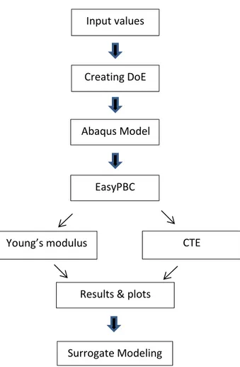
3. METHOD AND IMPLEMENTATIONS

There were six steps to focus on this project which are as follows: • Abaqus Model

• Python Implementations • Making DoE from Inputs • Connecting DoE with Abaqus • Compiling Results and Plot

• Computing surrogate model coefficients (beta) Input values

Abaqus Model

Young’s modulus

Surrogate Modeling

Figure 9: Flowchart shows complete methodology and implementation of this project Creating DoE

CTE EasyPBC

(25)

3.1 Abaqus Model

First, a 3D cube model of graphite, ferrite, pearlite is created as shown in figure 10 below and meshed it. As the meshing is an integral part of the simulation. In which geometries of material are divided into small and simple elements so can be utilized as an individual separate approximation of large elements. This cube has two spheres with the same center. The three sections i.e. cube represent pearlite, the small sphere represents graphite, and the thickness is represented by ferrite as shown in figures 10 and 11.

(26)

To control the parameters of the Abaqus model a script was generated. In the script, functions were made so that using variables the input parameters could be changed controlled based on the requirement of the user. A part of the script is shown in figure 12. The variables in figure 12 like, YmGr represents Young’s modulus of graphite, PrGr represents Poisson’s ratio of graphite, and so on.

def model(YmGr,YmFe,YmPe,PrGr,PrFe,PrPe,RaGr,TkFe,VFGr,VFF,NoOfExp): #####...Gr...#####

YMGr = float(YmGr) # YM = Young’s modulus PrGr = float(PrGr) # Pr = Poisson ratio

TCGr = 60E3 # TC= Thermal conductivity PiGr = 2.26E-9 # Pi = Density

CTEGr = 8E-6 # CTE = Coefficient of thermal expansion CpGr = 720E6 # Cp = Specific Heat

#####...Fe...##### YMFe = float(YmFe) PrFe = float(PrFe) TCFe = 5E3 PiFe = 5E-9 CTEFe = 11E-6 CpFe = 750E6

#####...Pe...##### YMPe = float(YmPe) PrPe = float(PrPe) TCPe = 28E3 PiPe = 1.1E-9 CTEPe = 10E-6 CpPe = 830E6 ############

FRGr = float(VFGr) #VF= Volume friction FRFe = float(VFF)

############

GrRa = float(RaGr) #Ra= Radius #############

FeTk = float(TkFe) ) #Tk= Thickness ############

(27)

3.1.1 EasyPBC

EasyPBC is written in the Python programming language using ABAQUS commands. To make the module accessible in the ABAQUS CAE interface, the code is essentially positioned in the Abaqus plugin catalog before fire up. The module runs two principle stages to appraise the homogenized versatile properties by actualizing ideas of brought together occasional RVE homogenization strategy, these are the pre-handling and post-preparing stages. The principal stage decides RVE's mathematical measurements, distinguishes limit surfaces, makes nodal sets, makes hub to-hub imperative conditions, and applies the necessary relocation limit conditions. Though the post-preparing stage handles pressure strain counts and different tasks identified with assessing the versatile properties. EasyPBC requirement conditions are mostly separated into two sets: Young's moduli (and Poisson's proportions), and shear moduli. The code makes these two arrangements of imperative conditions dependent on required homogenized properties, where the various moduli are actualized by changing applied relocations on explicit reference focuses through limit conditions [16].

3.2 Python and Implementation

Python is used as a programming tool to develop a methodology to generate surrogate model coefficients for parametrized. There are many libraries, available, on Python and every library has a different purpose and offers different functionality. Therefore, the following libraries of Python were used for this thesis,

• pyDOE2 • Pandas • NumPy • Matplotlib 3.2.1 PyDOE2

The pyDOE2 bundle is intended to enable the researcher, to build, analyze, and so forth, to develop suitable exploratory plans. The bundle presently incorporates capacities for making plans for quite a few components:

1. Factorial Designs

• General full factorial • 2-level full factorial • 2-level fractional factorial • Placket-Burman

(28)

• Box-Behnken • Central-Composite 3. Randomized Designs

• Latin-hypercube 3.2.2 Pandas

Pandas is a library of Python computer language which offers a wide range of features, that provides a fast, customizable, and customizable database design with simple, personalized data management (same, multiple formats, perhaps different). It expects to be the essential elevated level structure block for doing functional, genuine information examination in Python. There are some main features of Pandas Python library

• Writing and reading file data in any format

• Providing a data frame object for given data with indexing • Joining and merging data

• Handling missing data and arranging data 3.2.3 NumPy

NumPy is a Python library utilized for working with arrays. It likewise has capacities for working in straight polynomial math, Fourier change, and networks. NumPy was made in 2005 by Travis Oliphant. It is an open-source undertaking, and you can utilize it unreservedly. NumPy represents Numerical Python. NumPy intends to give a cluster object that is up to 50x quicker than customary Python records. The cluster object in NumPy is called an array, it gives a great deal of supporting capacities that make working with an array exceptionally simple.

3.3 Making DoE from Input

The input excel file contained information about all required input for this thesis. Only 10 input parameters were considered which were based on the volume fractions of graphite and ferrite, Young’s modulus, and Poisson’s ratio of graphite, ferrite, and pearlite, a radius of graphite, and thickness of ferrite. Each input parameter has three different values, lower value, higher value, and center value. While all thermal inputs were not considered in this thesis, which was CTE, thermal conductivity, specific heat, and density of all three graphite, ferrite, and pearlite. The input file is shown in table 2.

(29)

Table 2: Input values

In table 2, YmGr, YmFe, YmPe represent Young’s modulus of Ferrite and Pearlite, respectively. PrGr, PrFe, PrPe represents the Poisson’s ratio of graphite, Ferrite, and Pearlite, respectively while RaGr and TkFe were the radius of graphite spheres and thickness of Ferrite in millimeter. The volume fraction of graphite and ferrite represents with VFGr and VFF respectively.

After reading the input data, creating a Box Behnken DoE layout was the next step. For the Box Behnken layout Python, the pyDOE2 library was used after obtaining the layout all input values were replaced into a layout and output a DoE which contains inputs values instead of -1,1, and 0. One row in DoE represents one experiment with different inputs.

3.4 Connecting DoE with Abaqus

Meanwhile, theDoE connected with the Abaqus model by the commands “import.os” and “import.sys”. This is because it will replace the input values in Abaqus automatically and generate results. The main reason to connect DoE with Abaqus is that all experimental values could be replaced automatically in Abaqus inputs and gives results. For connecting DoE with Abaqus two different scripts were needed:

1. One which based on the Abaqus model (Final-3D-one.py) 2. One script has DoE data (DoE and Abaqus.py).

In final-3D-one.py, “import.sys” was added at the top. This is to access the values of DoE which is being sent in the form of os.system ( ) called above via sys.argy[ ] shown in figure 13 and to send DoE value into os.system () using import os in DoE and Abaqus.py as shown in figure 14.

YmGr

(MPa) YmFe (MPa) YmPe (MPa) PrGr PrFe PrPe RaGr (mm) TkFe (mm) VFGr VFF Lower value 13000 192000 172000 0.3 0.29 0.28 0.35 0.06 0.3 0.2 Center value 13500 196000 176000 0.3 0.31 0.295 0.38 0.075 0.4 0.245 Higher value 14000 200000 180000 0.3 0.33 0.31 0.41 0.09 0.5 0.29 model(sys.argv[-11],sys.argv[-10],sys.argv[-9],sys.argv[-8],sys.argv[-7], sys.argv[-6],sys.argv[-5],sys.argv[-4],sys.argv[-3],sys.argv[-2],sys.argv[-1])

(30)

Figure 14: Sending input values in os.system and calling Abaqus

3.5 Compiling Results and Plot

At this level, results for each experiment were noted and concluded by desired Young’s modulus and Coefficient of thermal expansion (CTE) by reading every file. For instance, Abaqus will generate copies of results for every experiment which will be noted and helpful for gathering data.

Furthermore, after combining DoE with outputs and a plot of Young’s modulus and Coefficient of thermal expansion (CTE) in Python, the matplotlib library was used.

3.6 Computing Surrogate Model Coefficients

To find the value of the surrogate model coefficients (beta) for a quadratic surface response, equation (6) was used which is

𝛃 = (𝐗T_{. 𝐗)}−1_𝐗T_𝐲 ₍₇₎

Where 𝛃 is vector of surrogate model coefficients, X is matrix of independent variables and 𝐲 is vector of the observations in this thesis which are Young’s modulus and CTE.

X in equation (7) is matrix of inputs values described as So, X can be simplified as

X = [1 DoE (DoE)2_] ₍₁₎

os.system("abaqus cae nogui=Final-3D-model.py -- " + str(iput[0]) + " " + str(iput[1]) + " " + str(iput[2]) + " " + str(iput[3]) + " " + str(iput[4]) + " " + str(iput[5]) + " "+ str(iput[6]) + " " + str(iput[7]) + " " + str(iput[8]) + " " + str(iput[9])+ " " + str(i))

1 x_1x1 x_2x1… … …. x_10x1 x_1x12 x_2x12 … … … x_10x12 1 x_1x2 x_2x2… … … x_10x2 x_1x22 x_2x22 … … … x_10x22 X= . . . . . . . . 1 x_1x190 x2x190… … … x10x190 x1x1902 x2x1902 … … … x10x1902 (8) DoE

(31)

3.7 Working Procedure The steps for using the script,

1. Change input values in the input excel file which is with the script file and keep both files at the same location.

2. Install four libraries in Python, pyDOE2, Pandas, NumPy, and Matplotlib.

3. Link EasyPBC with Abaqus and then make some changes in the Abaqus script as mentioned in figures 13 and 14.

After following the above steps, the script can be run to obtain the result. All result excel files will generate in the same directory.

(32)

4. RESULTS

4.1 Abaqus Results

First, a text file of each experiment was gathered which contain all the useful information by running Abaqus. A total of 190 experiments were performed with 10 inputs, then 190 copies of text files containing data for each experiment is obtained. The results obtained were in three-dimensional (x,y, and z), to be precise, the first three rows illustrate Young's modulus in possible three dimensions while the next three rows illustrate the Shear modulus in the three-dimensions.

Lastly, rows from 7 to 12 represent Poisson’s ratio in six directions xy, xz, yx, yz, zx, and zy, while the Coefficient of thermal expansion (CTE) from 13 to 15. For instance, table 3 is showing the text file of the very first experiment which is experiment 0. Table 3 describes the detail about parameters in terms of name, unit, and values which were obtained from Abaqus.

Table 3: Detail information about the Abaqus output file

Sr. No Name Value Unit

1 Young's modulus(x) 125662.14 MPa 2 _{Young's modulus(y)} _125661.04 _MPa 3 _{Young's modulus(z)} _125661.78 _MPa x _{Shear modulus (x)} _44671.25 _MPa 5 _{Shear modulus (y)} _44671.01 _MPa 6 _{Shear modulus (z)} _44671.02 _MPa 7 _{Poisson's ratio (xy)} _0.27 _ratio 8 _{Poisson's ratio (xz)} _0.27 _ratio 9 _{Poisson's ratio (yx)} _0.27 _ratio 10 _{Poisson's ratio (yz)} _0.27 _ratio 11 _{Poisson's ratio (zx)} _0.27 _ratio 12 _{Poisson's ratio (zy)} _0.27 _ratio 13 _{CTE (x)} _-0.00001 _mm 14 _{CTE (y)} _-0.00001 _mm 15 _{CTE (z)} _-0.00001 _mm 16 _{Total mass} _2.01E-09 _{tonne(1000kg)} 17 _{Homogenised density} _2.01E-09 _tonne/mm3 18 _{Processing duration} _359.12 _second

(33)

Table 3 shows the homogenized material parameters of SGI for the RVE which are isotropic since Young’s modulus in the x,y, and the z-axis are the same(E1=E2=E3) and the CTE in all three axes is also the same. This is because all phases are isotropic, and the geometry of the microstructure is symmetric that’s why the deformation will be the same in all three directions.

4.2 Creating Box Behnken Layout and Replace with Values

A standard layout of the Box Behnken DoE (BBD) was created using Python which only consists of three values -1, 0, and 1 as shown in table 4. Where -1 and 1 represent lower and higher points while 0 represents the center point of inputs. Later all three values are replaced by the required input value from the original input file. The final BBD shown in table 5. A total of 190 experiments were created out of the 10 inputs and only first 14 experiments were shown in this report.

Table 4: The Box Behnken DoE layout

(34)

To obtain the total number of experiments equation (3) can be used for given inputs. The number of inputs (k) is 10 and thus the number of control factors (center points, C0) would

be 10. Thus equation (3) now becomes,

N=2*10(10-1) +10=180+10=190

Thus, the total number of the experiments would be 190, which were created in this section. 4.3 Computing Output Values

A copy of the experiment results from Abaqus was created as shown in table 3 and imported in Python, to obtain the desired data from the experiments. As the thesis revolves around Young’s modulus and Coefficient of thermal expansion(CTE), at this level it is only required to read Young’s modulus and CTE from table 3, rows from 1 to 3, and rows 13 to 15 respectively. The average value of both the variables i.e. Young's modulus and CTE were concluded, thus two output values for each experiment can be obtained as shown in table 6.

Table 6: The homogenized average values of Young's modulus and CTE

AvgYm (MPa) AvgCTE(mm)

Exp-0 125661.6601 -0.00001 Exp-1 126126.2044 -0.00001 Exp-2 126751.9759 -0.00001 Exp-3 127214.3652 -0.00001 Exp-4 124081.8326 -0.00001 Exp-5 124543.1770 -0.00001 Exp-6 128329.7981 -0.00001 Exp-7 128795.3255 -0.00001 Exp-8 126208.9583 -0.00001 Exp-9 126672.4218 -0.00001 Exp-10 126208.9583 -0.00001 Exp-11 126672.4218 -0.00001 Exp-12 126076.1914 -0.00001 Exp-13 126541.5201 -0.00001

The average Young’s modulus values are varying while the average CTE values are constant in the experiments which can be seen in table 6, this is because thermal parameters were considered to be constant for the development of the script.

4.4 Combine DoE with Output

The script combines the DoE and output values in the form of an output file so that the researcher/user can get everything under one file for better visualization of the results concerning the inputs. Table 7 showing that the experiment from 0 to 13; and the output of

(35)

different experiments along with their average Young’s modulus and average CTE in each row.

Table 7: Combine DoE with output values

4.5 Computing Surrogate Model Coefficients

To find the surrogate model coefficient (beta) for the true surface response the equation (7) and equation (9) were used. A total of 21 beta values were gathered which contains two beta columns, one for Young’s modulus and the other for the coefficient of thermal expansion(CTE). Further, these two values can be used to find an optimized solution.

Table 8: Beta values of Young’s modulus and CTE

Ym-Beta CTE-Beta Beta-1 −171762 −3𝑒−6 Beta-2 4.72 −1.1𝑒−17 Beta-3 1.14 −3.2𝑒−18 Beta-4 1.46 −7.9𝑒−19 Beta-5 2148.99 7.3𝑒−6 Beta-6 44634.23 1.2𝑒−13 Beta-7 80041.98 2.86𝑒−13 Beta-8 -359422 1.12𝑒−13 Beta-9 -314911 9.39𝑒−14 Beta-10 3128.76 5.56𝑒−15 Beta-11 9463.52 1.6𝑒−14 Beta-12 −0.0001 −6.1𝑒−23

(36)

Beta-15 910782.1 −1.1𝑒−4 Beta-16 −60126.2 −2.9𝑒−13 Beta-17 −139469 −5.9𝑒−13 Beta-18 63022.9 −1.1𝑒−13 Beta-19 2618866 −4𝑒−13 Beta-20 −3910.95 −6.2𝑒−15 Beta-21 −19313.3 −2.7𝑒−14

There are two outputs, the average Young’s modulus, and the average CTE values and thus two different surrogate model coefficients (beta) are obtained by using equation (7). There is a significant difference between Young’s modulus beta values and CTE beta values. CTE beta values are too small as compared to Young’s modulus values.

After getting beta values for Young’s modulus and CTE response, the approximate model for the true surface response for Young’s modulus and CTE can be obtained by using equation (5).

𝑓(x) = β₀+ β₁x₁+ β₂x₂… … + β₁₀x₁₀+β₁₁x₁2+β₁₂x₂2+β₁₃x₃2… … +β₂₀x₁₀2 (2) so, for two response, two models will be obtained which are

• Model for the true surface response for Young’s modulus,

𝑔(x) = −171762 + 4.72x₁+ 1.14x₂+ 1.46x₃+ 2149x₄ + 44634.23x₅+ 80042x₆− 359422x₇− 314911x₈ + 3128.76x₉ + 9463.52x₁₀− 0.00016x₁2− 2.6e−6x₂2 − 2.6e−6_x 3 2_{+ 910782.1x} 42− 60126.2x52− 139469x62 + 63022.9x₇2+ 2618866x₈2− 3910.95x₉2− 19313.3x₁₀2 (3)

• Model for the true surface response for CTE,

ℎ(x) = −3e−6− 1.1e−17x₁− 3.2e−18x₂− 7.9e−19x₃+ 7.3e−6x₄ + 1.2e−13_x

5+ 2.86e−13x6+ 1.12e−13x7+ 9.39e−14x8

+ 5.56e−15x₉ + 1.6e−14x₁₀− 6.1e−23x₁2− 3.1e−24x₂2 + 2.57e−24_x

32− 1.1e−4x42− 2.9e−13x52− 5.9e−13

− 1.1e−13_x 7 2_{− 4e}−13_x 8 2 _{− 6.2e}−15_x 9 2_{− 2.7e}−14_x 10 2 (4)

(37)

5. DISCUSSION

To obtain the required goals for developing a methodology to generate surrogate model coefficients for the parametrization of SGI, Abaqus, and Python were used. There are some merits and demerits which will discuss in this section. The results demonstrate that the script will generate surrogate model coefficients (beta) from input values. Later these inputs values were used to generate a DoE and linked with Abaqus for obtaining homogenized parameters that were used to generate the required result.

For a simple understanding of the script, a simple Abaqus model with default settings and EasyPCB was used. An Abaqus model script is generated and linked with the main script. This simple Abaqus model can be replaced by any complicated and more detailed Abaqus model with the same number of inputs and linked with the main script. The linking with the main script is as mentioned in figures 13 and 14.

The surface response can be found through two methods i.e. Box Behnken Designs and Center Composite. We choose the Box Behnken method because it has saved us much time as compared to the Center Composite method; Because Center Composite is a full factorial method and is denoted by NK_{, Where K is the number of levels and N is the number of inputs.}

In this thesis, we took 10 inputs, if we use the Center Composite method, we must have to deal with a larger number of experiments.

Table 6, showing the Young’s modulus varies as we consider different volume fraction inputs for different experiments whereas the CTE values remain constant as we consider constant thermal inputs for all the experiments.

The visualization of the Pareto optimal solution is typically between two different functions, which varies from point to point. In this thesis, there are two different output values (Young’s modulus and CTE) where CTE values are constant while Young’s modulus values vary as per the experiment. This why the visualization of the Pareto optimal solution is not possible with the given input values. If the CTE values change with the experiment, then the same script will be able to generate a Pareto optimal solution plot. For the CTE values to vary, the thermal inputs need to vary.

This script could help people to design a better product without having to spend much time on changing material input parameters for every experiment or running a finite element analysis on each case. By using this script, they just need to set the input parameters in an Excel file and then run the script. The solution will be automatically generated as an excel file with all the necessary information once the finite element analysis is complete.

(38)

6. CONCLUSIONS

From the above observation, it can be concluded that the script can be applied to optimize the performance of the microstructure of SGI. The developed script connects a 3D Abaqus model and has the ability to visualize a Pareto optimal solution. One can enter all the input values in an Excel file and the script generates a DoE based on the number of inputs. The DoE is connected with Abaqus which computes homogenized Young’s modulus and the CTE for each of the experiments. The script is able to use Young’s modulus and CTE values obtained to visualize a Pareto optimal solution and beta (surrogate model coefficients) if the correct CTE values are used in the input. The output Excel files (DoE file, DoE combined with output and beta value file) with all the necessary information and a plot of Young’s modulus and CTE is obtained which is easily understandable and usable by the user. Further, the beta values can be used in the necessary polynomial equation (10) to obtain the true surface response model and that model can use to find the optimal solution.

(39)

7. FUTURE WORK

There are two future work recommended after working on a thesis for improvement and further research

7.1 Increment in Inputs

For this thesis, only volumetric fraction-related inputs were considered which varies only Young’s modulus value while CTE values were almost constant in every experiment. To improve the accuracy of the results, factors influencing the CTE values like the thermal parameters and density can be considered in the script.

7.2 Optimization

The equation (11) and (12), the polynomial expression obtained from the surrogate model coefficients beta, solving on which one can obtain an optimal solution for the given problem.

(40)

8. REFERENCES

1. B.L. Bramfitt and A.O. Ben scoter, Metallographer's Guide: Practices and Procedures for Irons and Steels, USA, 2002, ASM International, Chapter 1, page 16-21

2. AVNER Sidney H, Introduction to Physical Metallurgy, Second Edition, MCGRAW HILL INTERNATIONAL EDITIONS, chapter 11, page 450-453

3. C. Bach and R. Baumann, Elasticitat und Festigheit, 9th ed. (Julius Springer, Berlin, Germany, 1924).

4. Handbook On Design Engineers Digest On Ductile Iron, Eighth Edition, IBM, West Germany

5. James H Davidson, Microstructure Of Steel And Cast Irons, New York, Springer-Verlag, 2003, ISBN 3-540-20963-8, Part 3, Chapter 21, Page 356-363

6. Ductile.org. 2020. Ductile Iron Data - Section 2. [online] Available at: <https://www.ductile.org/didata/Section2/2intro.htm> [Accessed 9 September 2020]. 7. Ductile Cast Iron – IspatGuru at:

<https://www.ispatguru.com/ductile-cast-iron/>[Accessed 10 September 2020].

8. Dieter Goerge E., Mechanical Metallurgy, Adapted by David Bacon, McGraw-Hill Book Company, Materials Science & Metallurgy Series, SI Metric Edition, ISBN: 0-07-100406-8 9. Exploring the Stress / Strain Curve for Mild Steel - The Chicago Curve

<https://www.cmrp.com/blog/faq/analysis-design/exploring-stress-strain-curve-mild-steel.html/>[ Accessed 9 November 2020].

10. Rodriguez, F., Boccardo, A., Dardati, P., Celentano, D., and Godoy, L., 2018. Thermal expansion of a Spheroidal Graphite Iron: A micromechanical approach. Finite Elements in Analysis and Design, 141, pp.26-36.

11. Ahmed Ibrahim Badr, 2014. “ General introduction to Design of Experiments (DOE)” 12. S.L.C Ferreira. Et.all 2007. “Box-Behnken Design: An alternative for the optimization of

analytical methods” 179-186

13. Forrester, Sobester & Keane (2008), “Engineering Design via Surrogate Modelling: a practical guide”, Wiley, Southampton, UK

14. Myers Raymond H. & D.C. Montgomery, 2002. “Response Surface Methodology: process and product optimization using designed experiment,.” A Wiley-Interscience Publication. 15. Tanaka, M., 2003. Inverse Problems In Engineering Mechanics IV. 4th ed. Elsevier

Science, pp.90-95.

16. Sadik L. Omairey, Peter D. Dunning & Srinivas Sriramula, 2018. “Development of an ABAQUS plugin tool for periodic RVE homogenization”

17. What is Ductile Iron at: <http://www.wb-machinery.com/what-is-ductile-iron.html>[Accessed 9 September 2020].

18. Kathleen M. Carley, Natalia Y. Kamneva, Jeff Reminga,2004. “Response Surface Methodology”, pg 1-6