Searching for atmospheric signals in states of low Antarctic sea ice concentration

Searching for atmospheric signals in states

of low Antarctic sea ice concentration

Meteorological Institute, Stockholm University

MO9001 - Degree Project

Aiden J¨

onsson

Supervisors

Frida Bender

Meteorological Institute, Stockholm University

Abhay Devasthale

Swedish Meteorological and Hydrological Institute

5 October 2018

Abstract

The Antarctic sea ice region is relatively stable in extent from year to year and sees little long-term variability, the primary driver for its seasonal advance and retreat being the seasonal changes in advection of heat through the atmosphere. However, observations show a slight positive trend in its extent over recent decades. Recent work has built on the hypothesis that anomalous poleward moisture fluxes could be seen in concert with anomalous decreases in sea ice variability by providing evidence of this correlation in the Arctic sea ice region. In order to test this hypothesis and to investigate the atmospheric circulation patterns during states of low sea ice concentration in the Antarctic, records of de-seasonalized sea ice concentration anomalies are made for five regions of the Antarctic polar region, and composite distributions of variables of atmospheric circulation for the lowest 10th _{percentile of months with low mean sea ice concentration are compiled.}

Merid-ional moisture fluxes from these composites are tested against the entire population of meridional moisture fluxes using the Student’s t-test with a confidence level of 95%, and the differences from the overall mean fields for atmospheric conditions during these cases are calculated. Of the five regions, the Ross Sea, Weddell Sea, and Pacific Ocean sections exhibit significant local moisture flux anomalies in the direction of the pole during months with low sea ice concentration, supporting the hypothesis that moisture transport into the polar region is important for the variability of sea ice in the Antarctic. The Bellingshausen - Amundsen Seas and Indian Ocean sectors show weak local signals of poleward moisture fluxes, indicating that there are other varying factors affecting the sea ice more heavily in these regions. Mean geopotential height anomalies during months with anomalously low sea ice concentration indicate that the Weddell Sea and Pacific Ocean regions are coupled with the positive phase of the Southern Annular Mode, while low sea ice concentration in the Indian Ocean as well as the Bellingshausen and Amundsen Seas regions show concur-rence with the negative phase. With general circulation models predicting a persistence of the positive phase of the Southern Annular Mode in a warming climate, it is important to understand how the Antarctic sea ice region responds to the phase of this oscillation.

Acknowledgements

To MISU, the most welcoming institution I’ve ever been a part of, and all of the bright and passionate souls there who work so hard there. To the authors of the OSI-450 database for producing a truly remarkable tool for studying sea ice, and for giving patient, positive and constructive answers to questions about their work. A great thanks to my supervisors: to Frida, for being a compassionate, supportive supervisor and motivating me at every step to carry out quality work, and to Abhay, for sharing his inspiring knowledge and enthusiasm for the subject of this project, and for his skillful analyses along the way. To my dad, for encouraging and aiding me along the road to reach the end of the masters degree. To Danielle, for being by my side throughout every step of the process, reminding me to eat while writing, and working together with me to make our home a safe and relaxing place to carry out my studies.

Contents

1 Introduction 4

2 Methodology 10

2.1 Sea Ice Concentration . . . 10

2.2 Historical Reanalysis . . . 13

2.3 Calculations and Data Processing . . . 14

3 Results 16 4 Discussion and Conclusions 29 4.1 Discussion . . . 29

4.2 Limitations . . . 31

4.3 Societal Implications . . . 33

4.4 Conclusions . . . 35

Glossary of abbreviations

BS: Bellingshausen and Amundsen Seas region

DMSP: Defense Meteorological Satellite Program

ECMWF: European Center for Medium-Range Weather Forecasts

ENSO: El Ni˜no-Southern Oscillation

ERA: ECMWF Reanalysis

EUMETSAT: European Organization for the Exploitation of Meteorological Satel-lites

GCM: General Circulation Model

IO: Indian Ocean region

OSI SAF: Satellite Application Facility on Ocean and Sea Ice

PO: Pacific Ocean region

RS: Ross Sea region

SAM: Southern Annular Mode

SH: Southern Hemisphere

SIC: Sea Ice Concentration

SO: Southern Oceans

VINMF: Vertically Integrated Northward Moisture Flux

WS: Weddell Sea region

Section 1

Introduction

The polar regions are expected to experience the greatest change in climate relative to lower and middle latitudes with a globally warming climate. This effect – which has been dubbed polar amplification – is predicted early on by models in the IPCC 1990 report (Chapman and Walsh, 1993) and that is continuing to gain observational evidence. The differences in climate responses between lower and higher latitudes is expected to be most evident in the Arctic polar region, which has seen the greatest warming of any region on the planet; in direct contrast, a quickly warming climate is not seen in the Antarctic (Collins et al., 2013). The dominant factors controlling the difference between the two hemispheres’ polar regions are widely believed to be the mixing of heat into deep waters in the Southern Oceans (Marshall et al., 2014), the ice sheet’s persistence on the land mass (Pachauri et al., 2014), and the surface height and orography on the continent (Salzmann, 2017), although all possible causes have not been investigated or quantified.

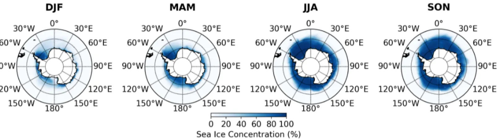
Figure 1.1: Seasonal average Antarctic sea ice concentration fields for the years 1982-2010 (DJF: December-January-February, MAM: March-April-May, JJA: June-July-August, SON: September-October-November).

The sources of heat in the Antarctic polar region also differ greatly from the Arc-tic. The Arctic region’s heat budget is highly dynamic and shifts heavily throughout the seasons: during the fall and winter, the Arctic Ocean adds heat to the atmosphere as radiative solar heating subsides, and when radiative solar flux begins to increase during spring and summer, the atmosphere’s heat energy continues to increase while the ocean begins to gain heat from the atmosphere (due to the melting of sea ice and increased radiative heating from the subsequently lower albedo) (Serreze et al., 2007). Advection of heat into the Arctic polar region by atmospheric circulation is quite low. In the Antarctic, downward vertical motion from the stratosphere transports most of the heat, while hori-zontal eddies transport about 3 to 5 times less heat into the region (Rubin and Weyant, 1963); the primary contributors to observed temperature changes between seasons are increased warm air advection and sea ice melt, and the stratosphere and troposphere are radiatively cooled at all times of the year. The Antarctic sea ice region is annually consis-tent in exconsis-tent and variations are relatively small: most of the Southern Ocean is ice-free during southern hemisphere (SH) summer months and reaches a minimum in February. For the maximum sea ice extent, there is little variability from year to year despite a very slightly positive positive trend in recent decades: + 1.0 ± 0.4% during the years 1979 to 2006 (Cavalieri and Parkinson, 2008)(Macalady and Thomas, 2017). This is in contrast to the Arctic, which is experiencing a strong negative trend in sea ice extent at - 3.4 ± 0.2% per decade (Comiso and Nishio, 2008)(Stroeve et al., 2007). Despite modest trends in the Antarctic, the region’s stability and lower variability of sea ice from year to year may allow for the possibility of a clearer picture of meteorological variables’ effects on sea ice with less difficulty in removing any signals of long-term trends.

A narrow band near the coast of the Antarctic continent that comprises only 1.5% of the total Antarctic sea ice region’s surface area at the maximum is responsible for nearly all of the formation of sea ice in the southern hemisphere (Massom and Stammerjohn, 2010). As well as the production of sea ice, much of the formation of Antarctic Bottom Water occurs within this area, making processes near the coast crucial and far-reaching in effects on the circulation of the world’s oceans. In the coastal zone, sea ice formation is controlled mostly by the interface between the ocean and the continental ice sheet and ice bergs, the seasonal change in temperature, as well as katabatic winds over the continent. These katabatic winds affect sea ice production by transporting newly formed, unpacked

ice away from the coast; strong, sustaining katabatic winds more perpendicular to the coast are associated with high sea ice production (Massom et al., 2001). The process of seasonal melt in the entire sea ice is affected by the atmospheric processes during the melt season. Primarily, heat advection during the onset of spring sets the stage for the melting of winter sea ice, and speeding the process of melting is the breaking of the sea ice pack by storms. The frequency of cyclones in the region as well as wind speeds during winter months are negatively correlated with maximum sea ice thickness (Heil, 2006). Aside from the mechanical breaking of sea ice by high wind speeds, storm-induced ocean swells cause further fragmentation and may cause breakage even beyond the storm path (Langhorne et al., 2001). Although there is not much year-to-year variability in the seasonal cycle of Antarctic sea ice, there are slight changes in the cycle currently being observed: the date of the sea ice maximum (defined as the reaching of a maximum thickness of the ice sheet) is delayed by 0.43 days per year (Heil, 2006). This change is attributed to increased mean winter- and springtime temperatures.

Coupled with cyclone activity in the southern polar region is increased moisture transport into the region (Grieger et al., 2018). Several papers in recent years have worked with the hypothesis that moisture transport events into the Arctic are an im-portant factor in affecting and determining sea ice concentration and extent (Johansson et al., 2017)(Yang and Magnusdottir, 2017); water vapor intrusions (WVIs), anomalously high influxes of moisture into the region, are shown to be correlated with negative sea ice anomalies in the Arctic. WVIs can set the conditions for accelerated sea ice melt in many ways, beginning with the direct radiative effect: water vapor is by far the dominant greenhouse gas in Earth’s climate (Held and Soden, 2000). Water vapor in the atmo-sphere affects radiation balance in the atmoatmo-sphere by absorbing and re-emitting longwave radiation; global climate is more sensitive to water vapor than to carbon dioxide in this respect (0.125 C per W m−2 versus 0.023 C per W m−2 after measurements made in Stan-hill, 2011). Long-wave radiation in the infrared spectrum is absorbed and re-emitted by water vapor, increasing the downwelling radiative flux and trapping the energy within Earth’s atmosphere.

On top of water in the form of vapor acting as a greenhouse gas, there is also the possibility that clouds will form, affecting how the presence of moisture affects the sea ice region. The formation of clouds complicates the understanding of climate significantly;

the greatest amount of disagreement between general circulation models (GCMs) is found to be due to the interactions of clouds with climate (Stephens, 2005). Cloudy, humid atmospheric conditions absorb and re-emit long wave radiation, the downward component of which creates a warming effect largely during the winter when long wave radiation is being emitted by the Earth and incoming solar radiation is decreased (worse conditions for sea ice formation or persistence). When there is incoming solar radiation, optically bright clouds reduce incoming short wave radiation and thereby have a cooling effect – which may retard the retreat of sea ice. With these effects combined, the greatest effect of cloudy conditions upon sea ice occur during spring and summer: downwelling short wave radiation anomalies affect sea ice only after the onset of melt, while downward long wave radiation anomalies affect sea ice significantly during spring and summer (Kapsch et al., 2016). Increased downwelling radiation in both short and long wavelengths do not significantly affect sea ice during the winter.

There are also several known related feedback mechanisms that affect the climate of the polar regions. As temperatures increase, the melting of sea ice decreases the surface albedo of the region, which increases the absorption of incoming shortwave solar radiation, thus raising the temperature; this surface albedo feedback can be characterized in a simple model of energy balance (Thorndike, 1992). The model shows that the polar regions are unstable and can shift abruptly from ice-covered to ice-free due to this feedback. As ice melts, the increased open water surface area allows for increased evaporation, which increases locally sourced moisture and potentially precipitation in the region; in the Arctic, this mechanism is measured to have a direct effect of an 18.2 ± 4.6% and 10.8 ± 3.6% increase in regionally sourced moisture in the Canadian Arctic and Greenland Sea, respectively, for every 100,000 km2 _{of sea ice lost (Kopec et al., 2016). Another}

mechanism affecting the complex climate dynamics of the sea ice region is the enhanced ability of air to retain moisture as temperature increases, leading to further warming and moisture retention in the atmosphere; this effect, known as the water vapor feedback, makes for an estimated radiative forcing of + 2.04 W m−2K−1 (Dessler et al., 2008).

Some studies have sought to quantify the moisture fluxes and pinpoint their sources using reanalysis; ERA-40 satisfactorily fulfills hydrological balance in the Antarctic polar region, and there is no significant trend in moisture flux or precipitation despite large variability (Tiet¨av¨ainen and Vihma, 2008). Inter-annual variations in zonal moisture

transport are positively correlated to the Antarctic oscillation or Southern Annular Mode (SAM). The Antarctic is found to have a year-round stationary poleward inflow of mois-ture off of the Antarctic Peninsula, and a seasonal inflow through the Amundsen and Bellingshausen Seas during fall and winter (Oshima et al., 2004) – a corridor that is analogous to the North Atlantic inflow of moisture into the Arctic region (Yang and Mag-nusdottir, 2017). There is evidence that the Antarctic Peninsula has been experiencing more warming than the rest of the Antarctic continent (Vaughan et al., 2003), which may have implications for the importance of the effects of water vapor in the Antarctic region in a globally warming climate.

Moisture transport into polar regions will increase in frequency and magnitude in a warming climate, making it yet another feedback in the global climate system that begs for understanding. While there are a number of studies on the balance of radiation and the role of moisture transport in sea ice variability in the Arctic, there are few investigat-ing how moisture transport affects the Antarctic sea ice region. Variability in poleward moisture flux in the Antarctic region is high, but there is currently no sign of a long-term trend (Tsukernik and Lynch, 2013), as opposed to the Arctic. This illustrates yet an-other way in which the Arctic and Antarctic are asymmetric in climate dynamics, and further understanding of the parameters that determine each polar region’s climatology is crucial for comprehensive knowledge about the global climate system. Here, it is hy-pothesized (following the work of Johansson et al. 2017) that when analyzing periods of low sea ice concentration in the Antarctic polar region, positive moisture anomalies can be seen in conjunction with its accompanying tropospheric circulation attributes. This study seeks to investigate historical cases of anomalously low SIC and how the variables in atmospheric circulation and meteorological conditions differ from the mean, in contrast to prior work on the same subject in the Arctic (Johansson et al., 2017) where the 90th

percentile cases of anomalously high poleward moisture flux were chosen as the start-ing point. In the Arctic, it was found that the anomalously high vertically integrated northward moisture flux (VINMF) showed a strong correlation with states of low SIC. While the circulation characteristics are different in the Antarctic polar region, a point of major interest in this study is how moisture and its transport is acting during states of low SIC. If the conclusions of Johansson et al. (2017) hold, then the results of this study should see a signal of positive moisture and moisture flux anomalies during time

periods with low SIC in the Antarctic – though they may not be purely poleward. Does moisture accumulate into anomalies in specific humidities during cases of low mean sea ice concentration? Are there certain humidity and temperature characteristics that are seen in conjunction with months of low mean sea ice concentration? This study will focus on answering these questions by investigating vertical profiles in both zonal and meridional directions as well as the specific humidity and temperature profiles. The hypothesis that positive moisture and moisture flux anomalies can be seen during states of anomalously low SIC in the Antarctic polar region will be tested, which would provide further evidence to the conclusions proposed by Johansson et al. (2017).

Section 2

Methodology

2.1

Sea Ice Concentration

The starting point of all analyses made in the study is the second version of the OSI SAF (Satellite Application Facility on Ocean and Sea Ice) Global Sea Ice Concentration Cli-mate Data Record, OSI-450, published by the European Organization for the Exploitation of Meteorological Satellites (EUMETSAT) (Norwegian and Danish Meteorological Insti-tutes, 2017). The record uses data from instruments aboard several satellites covering different timespans according to when they were launched: the Scanning Multi-channel Microwave Radiometer or SMMR (coverage: 1979 to 1987), Special Sensor Microwave Im-ager or SSM/I (1987 to 2008), and Special Sensor Microwave ImIm-ager/Sounder or SSMIS (2006-2015) (Lavergne et al., 2016). The Nimbus 7 satellite was launched in 1978 carrying the SMMR instrument, which was capable of measuring five frequencies with vertical and horizontal polarization. It was operated only every second day in order to conserve power, hence the availability of data only every other day during the first period of the OSI-450 data. As well as having lower sampling frequency than the subsequent instruments used for the dataset (which all had conical scanners), the SMMR is a forward-facing scanner covering a 780 km arc in front of the satellite with a surface incidence of 50.2° and a discrete sampling coverage of 25 km – this arc-shaped coverage makes the SMMR receiver more sensitive (giving more output per radiance received, reducing instrument noise and increasing accuracy) than conical receivers, which trade decreased radiometric sensitivity for more coverage and sampling. Because of this forward-facing setup and the incidence angle, there is no coverage poleward of 84°. Right before the SMMR stopped operating

in August 1987, the Defense Meteorological Satellite Program (DMSP) launched its first of six satellites with SSM/I instruments in July 1987. This conical scanner with a swath width of 1400 km had an incidence angle of 53.1° and a sampling resolution of 25 km for all but one channel (at 85.5 GHz, it was 12.5 km). This time, seven channels with varying polarizations measured four frequencies. The first instrument to be operated from 1987 malfunctioned along a crucial channel for a frequency necessary for calculating sea ice concentration, and thus the SSM/I data used in the OSI-450 database began in 1991. The final instrument to contribute to the OSI-450 database was the SSMIS, operated on three DMSP satellites. This instrument scanned a conical swath with a witdth of 1700 km and a constant incidence angle of 53.1°. Eight frequencies were measured in both polarizations on eight channels.

Several levels of algorithms were used on the raw data to produce the OSI-450 dataset. In the first level, the intensity of signal (brightness) from the 19 and 37 GHz channels with vertical polarization, and the 37 GHz horizontally polarized channel data was converted into a ratio of sea ice concentration within the scanned area. In the second level of algorithms used on the data, the data was corrected for land “spillover” effect in disrupted measurements of brightness taken within 50 km of the coast. This spillover effect is due to the coarse resolution of the scanning instruments used for retrieving the data; the reflectivity of land is higher than that of open water and therefore effects a false positive contribution to the brightness registered by individual pixels in the scanner. For this, the emissivity of the area sampled was divided into two components – sea and land – according to the fraction of land within the pixel from a geographic land-sea mask. Then, only the component from the sea area was used for subsequent steps. Still in the second level of processing, a hybrid of several types of algorithms weighed the outcomes of the calculations of sea ice concentration from the measured brightnesses in order to provide the most accurate possible calculation. The results of the calculations calibrated for correctness at 0% and those calibrated for 100% sea ice were multiplied by weighting factors (calculated during a tuning step) and summed by the algorithm. The difference in brightness values introduced by atmospheric conditions was added to correct for altered transmissivity in the atmospheric path using a radiative transfer model made with simplified radiation transfer equations (the creators of the OSI-450 database used Wentz 1983 for SMMR data and Wentz 1997 for SSM/I and SSMIS data). The

atmospheric parameters needed for this model included the air temperature at 2 meters, wind speed, and the total column water vapor content at the time of sampling; these were retrieved from ERA-Interim (Dee et al., 2011).

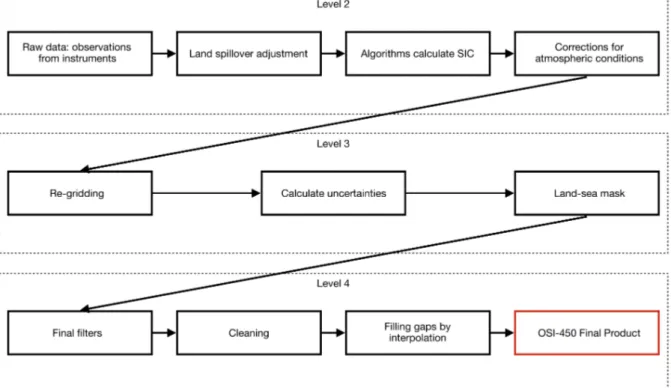
Then, in the third level of processing, the data was re-gridded, uncertainties were calculated for the data, and the land-sea mask was applied. In the fourth and final level of processing, “cleaning” for highly uncertain data points was carried out and any missing data was filled using interpolation. Yet more masks and filters were applied, including the climatological mask and the open water filter. The climatological mask removed values that are outside the maximum extent of sea ice for that year (which are defined to not be a part of the polar sea ice region, and therefore not of interest in the dataset). Some true sea ice may have been removed by the use of this filter, but the creators of the dataset believe that the threshold brought the database’s sea ice region closest to the true polar sea ice region. The open water filter was used to remove values calculated in earlier steps under a certain threshold that are most likely to actually be open water rather than a low concentration of sea ice. A visual representation of the process that was used in the construction of the dataset can be seen in Figure 2.1. The final product is a polar stereographic projection with a resolution of 25 km, a northernmost longitude of 40° S at the centers, and 16° S at the corners.

One difficulty experienced in the production of the OSI dataset was the sensing of melt ponds that lay on top of compacted sea ice during summer months. The sea ice con-centration in the dataset is computed as one minus the fraction of pixels detected as open water by the instrument, and so there are cases in the dataset where the concentration is not true due to the detection of water atop the ice. ”True” sea ice, in this case, refers to packs of ice afloat on the sea surface, whether there is water pooling on top of it or not. It is labor-intensive and difficult to discover ways in which meltwater contributions to SIC values can be excluded from the true sea ice. For the purpose of this study, it was determined to not be an issue as the primary focus is upon atmospheric variables that could be linked to decreased growth of sea ice as well as accelerated melting, both leading to negative anomalies in SIC as well as higher frequency of meltwater pooling on the top of the sea ice. Since the cases of interest are those of low sea ice concentration due to increased melt, including the occurrence of melt ponds, averaging a low concentration over a region due to the presence of melt ponds does not introduce problems.

Figure 2.1: Processing chain of converting satellite data to SIC data; simplified graphical description of the methods described in the OSI-450 manual (Lavergne et al., 2016).

2.2

Historical Reanalysis

For investigating atmospheric conditions, this study makes use of the most recent reanal-ysis dataset from the European Centre for Medium-Range Weather Forecasts (ECMWF), ERA-Interim (Dee et al., 2011). Reanalysis is a method used within atmospheric physics and climatology to construct a more spatially and temporally complete record of global weather and climate dynamics than observational data can provide. Satellite and in-situ data do not provide a complete record of weather and climate dynamics as there are gaps in time between data points collected while satellites make their passes over Earth, and in space, between observing stations. In reanalysis, observational data of atmospheric conditions are used in conjunction with forecast models based on prior observations in order to model past atmospheric states, and nudged in order to correct from error intro-duced in the forecast model; the observations make up the data assimilation step for this correction. In this way, gaps in data are filled in using extrapolation between points in the atmosphere, and forecast results from various timesteps are used to fill in gaps in time. The exact model used for ERA-Interim is ECMWF’s Integrated Forecast System (IFS), an atmospheric model first introduced in 2006 with 60 vertical pressure levels (the top

being 0.1 hPa) and a T255 spherical-harmonic spectral model of the Earth (256 latitudi-nal and 512 longitudilatitudi-nal elements), as well as with a coupled ocean wave model (24 wave directions and 30 frequencies at 1° × 1° resolution). The data product includes results at 3-hour intervals.

2.3

Calculations and Data Processing

All data records were downloaded in NetCDF format and manipulated using the Cli-mate Data Operators (CDO) set of command line operators (Max Planck Institute for Meteorology, 2018). The CDO program include different operations for ’mean’ and ’aver-age’: the ’mean’ is calculated excluding missing data and the ’average’ is calculated with missing data included. The ’mean’ operators were used for this study so as to disregard any missing data; though coverage is nearly complete in the datasets used for this study, the land-sea mask would introduce false contributions to the calculations if the masked numbers were not excluded.

The record of sea ice was first made into monthly means so as to use the larger array of reanalysis data in the monthly scale to investigate the climatology surrounding states of low sea ice concentration. A temporal resolution of monthly mean values was chosen due to the amount of information available in this format from ERA-Interim, allowing for a greater number of parameters to be investigated. The record of monthly means of sea ice was made into a record of de-seasonalized anomalies by calculating a mean annual cycle with monthly mean fields of sea ice concentration for the entire timespan, and then subtracting the corresponding month’s mean field from each individual month. The resulting record shows the differences from the mean climatology for that month, so that positive values represent an anomalous increase in sea ice concentration regardless of seasonality. Latitudes north of 53° S were excluded from the record in all calculations. The record spans a total of 408 months. In order to look at the regional circulation patterns and investigate the scale of moisture transport, mean anomalies were calculated for the fields within five sections of the Antarctic. These sections are: the Ross Sea (RS) (from 160° E to 130° W), the Amundsen and Bellingshausen Seas (BS) (130° W to 60° W), the Weddell Sea (WS) (60° W to 20° E), the Indian Ocean (IO) (20° E to 90° E), and the Pacific Ocean (PO) (90° E to 160° E). A total, region-wide field mean was calculated

to provide monthly records of average de-seasonalized sea ice anomaly for the five regions. To focus on the lowest sea ice cases, the bottom 10th _{percentile cases were selected from}

the time series of regional mean concentrations and collected into separate files for the low sea ice concentration states with a sample size of 41 cases for each region. Mean fields for these low sea ice concentration states were calculated for each region.

ERA-Interim records for monthly mean values of various fields were retrieved as monthly mean values for eleven pressure levels (1000, 925, 850, 700, 600, 500, 400, 300, 200, 150, and 100 hPa) at a 1° × 1° grid resolution. The parameters of primary interest were moisture flux, temperature (T ), zonal and meridional winds (u and v, respectively), geopotential height (φ), and specific humidity (q). These records of atmospheric variables were de-seasonalized into records of anomalies in the same fashion as the sea ice concen-tration record and composited for each region’s population of low SIC cases. In order to test the significance of the anomalies, a Student’s t-test was carried out on the fields of raw (not de-seasonalized) data from the two sample populations to calculate the probability that the distribution in the low SIC cases are different from the entire record’s distribu-tion. The non-de-seasonalized data was used because the process of de-seasonalization “normalizes” the values around a mean state, or zero (equal to the mean), and a t-test carried out on two populations centered around the same value will invariably lead to a false negative result. The areas where the data surpasses the confidence threshold of 95% were compared to the anomalies to confirm that the atmospheric variables were behaving significantly differently. Analysis of the atmospheric conditions corresponding to the low sea ice concentration cases was done using spatial plots of wind vectors and geopotential height anomalies, as well as vertical profiles of moisture transport (q times u for zonal moisture transport and q times v for meridional transport), specific humidity, and tem-perature along specific latitudes. Each of these variables’ anomalies from the mean field averaged over the months with low mean SIC were also plotted for an understanding of where and how they are different.

Section 3

Results

The starting point of the analysis in this study was to process the sea ice concentration data into de-seasonalized time series of regional means and determine the 10th _percentile

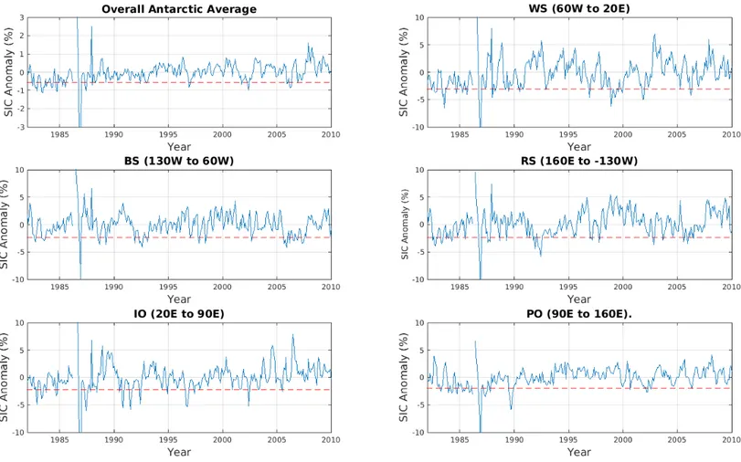
threshold where the lowest monthly mean SIC occur in each region, shown in Figure 3.1.

Figure 3.1: Time series of de-seasonalized monthly mean SIC anomalies calculated for the overall Antarctic polar region as well as over five sections (Weddell Sea: WS, Indian Ocean: IO, Pacific Ocean: PO, Ross Sea: RS, Bellingshausen and Amundsen Seas: BS), 1982-2010. Dashed lines represent the threshold for the 10th percentile.

The overall Antarctic average sea ice concentration sees variability on the decadal timescale, which is as expected from other analyses of observations (Fogt and Bromwich, 2006). The Indian and Pacific Ocean as well as the Weddell Sea regions show the least variation; these regions see low variability in moisture fluxes. The regional averages for the Ross, Amundsen and Bellingshausen Seas show the most variability, with possible trends on the decadal scale, agreeing with prior research (Oshima et al., 2004). In all regions, a spike occurs in 1986, a highly anomalous year with one of the lowest sea ice extents in the history of observations in the Antarctic (Stuecker et al., 2017).

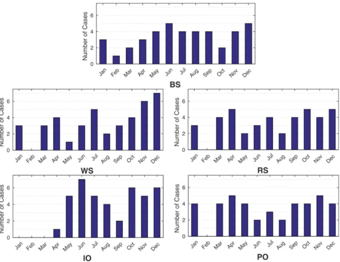
Upon selecting the cases from the bottom 10th percentile of SIC anomalies, it is useful to inspect which months are represented in the low SIC cases and be conscious of any implications of over- or underrepresentation when analyzing those conditions. Figure 3.2 includes bar charts with the number of cases in the 10th _{percentile of SIC anomalies}

in each month of the year.

Figure 3.2: Number of cases with the lowest (10thpercentile) monthly mean SIC anomalies in the composite distributions for each of the regions, divided into bins for the months of the year in which they occur (WS: Weddell Sea, IO: Indian Ocean, PO: Pacific Ocean, RS: Ross Sea, BS: Bellingshausen and Amundsen Seas).

The distribution of months included in each composite are satisfactorily comparable; if the cases were to fall unevenly into a narrow span of time, conclusions could only be drawn about that specific season. One can see that the SH summer months have a small share of cases with anomalously low SIC, as is expected due to the total retreat of sea ice. However, there is an even spread of the months in which sea ice is present.

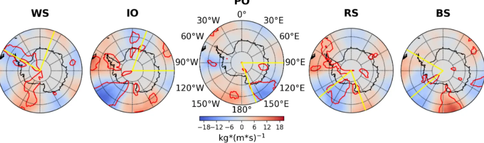
In Figure 3.3, the mean VINMF anomalies for the low SIC composite distributions of each region are plotted. The red contours show the areas where the distribution of absolute VINMF in the low SIC cases tested as significantly different from the entire sample population using the Student’s t-test with a confidence level of 95%.

Figure 3.3: Mean VINMF anomalies during months of low SIC; red contours show where the VINMF anomalies are different from the entire VINMF population at the 95% confi-dence level. The yellow longitudinal lines denote the boundaries of the section in each of the composites of low regional mean SIC (Weddell Sea: WS, Indian Ocean: IO, Pacific Ocean: PO, Ross Sea: RS, Bellingshausen and Amundsen Seas: BS).

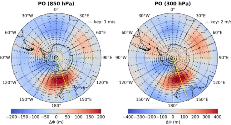
There are clear significant poleward moisture fluxes in the composite distributions of anomalously low SIC for the Weddell Sea, Pacific Ocean, and Ross Sea sections. A more complete view of atmospheric circulation during these cases is provided in Figures 3.4, 3.5, 3.6, and 3.7. In Figure 3.4, the total mean field of geopotential height and mean wind vector fields are plotted for the Antarctic region for the 850 and 300 hPa pressure levels. The average differences from the overall mean for the 850 hPa and 300 hPa pressure levels during the low SIC cases in each region are plotted in Figures 3.5, 3.6, and 3.7. The vector fields in each low regional mean SIC plot are therefore showing the small deflections in the direction of the average winds, not the absolute wind direction; plotting the deflections in monthly means as differences shows where circulation is shifted towards during the cases

Figure 3.4: Overall mean circulation characteristics: the mean geopotential height (φ) and the wind vector fields for the 850 hPa and 300 hPa pressure levels. Note that colorbars and vectors are scaled differently for each plot.

Figure 3.5: Differences from the overall mean circulation averaged over the 10th_percentile

of monthly mean sea ice anomalies within the Pacific Ocean (PO) section (west of 160° W and east of 90° W): the average mean geopotential height anomalies (∆φ) and the average difference in winds for the 850 hPa and 300 hPa pressure levels. Yellow meridional lines indicate the boundaries of the region. Note that colorbars and vectors are scaled differently for each plot.

(a)

(b)

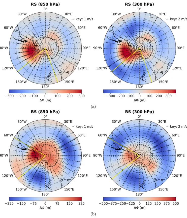
Figure 3.6: Differences from the overall mean circulation averaged over the 10th_percentile

of monthly mean sea ice anomalies within the Ross Sea and Bellingshausen/Amundsen Seas sections: the average mean geopotential height anomalies (∆φ) and the average difference in winds at the 850 hPa and 300 hPa pressure levels for (a) the Ross Sea (RS) region (west of 130° W, east of 160° E) and (b) the Amundsen and Bellingshausen Seas (BS) region (west of 60° E, east of 130° W). Yellow meridional lines indicate the boundaries of the region. Note that colorbars and vectors are scaled differently for each plot.

(a)

(b)

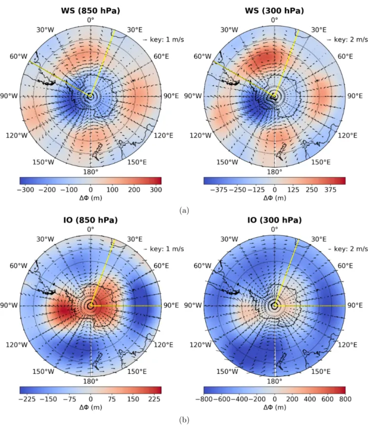
Figure 3.7: Differences from the overall mean circulation averaged over the 10th_percentile

of monthly mean sea ice anomalies within the Weddell Sea and Indian Ocean sections: the average mean geopotential height anomalies (∆φ) and the average difference in winds at the 850 hPa and 300 hPa pressure levels for (a) the Weddell Sea (WS) region (west of 20° E, east of 60° W) and (b) the Indian Ocean (IO) region (west of 20° E and east of 90° E). Yellow meridional lines indicate the boundaries of the region. Note that colorbars and vectors are scaled differently for each plot.

At both pressure levels, the Indian Ocean region exhibits a coastward and west-ward deflection of winds during months with low SIC, nearly exactly in the direction of the overall mean background wind field, meaning that the winds are braking by about half and weakening the mean circulation through the region. The mean state shows a northeastward flow in these regions, which would transport moisture out of the region; a braking could then cause moisture to remain in the region longer than usual. The Amund-sen/Bellingshausen Seas and the Ross Sea sections show a similar pattern with positive geopotential height anomalies above the continent and on the coast to the west of the Antarctic Peninsula. In the Ross Sea region, the positive geopotential height anomaly is greatly pronounced west of the Antarctic Peninsula, and wind is deflected zonally along the coast. In the Weddell Sea region, a geopotential height anomaly similar to that of the positive phase of the SAM is evident, which has been hypothesized to affect SIC in this region (Stammerjohn et al., 2008)(Yuan, 2004).

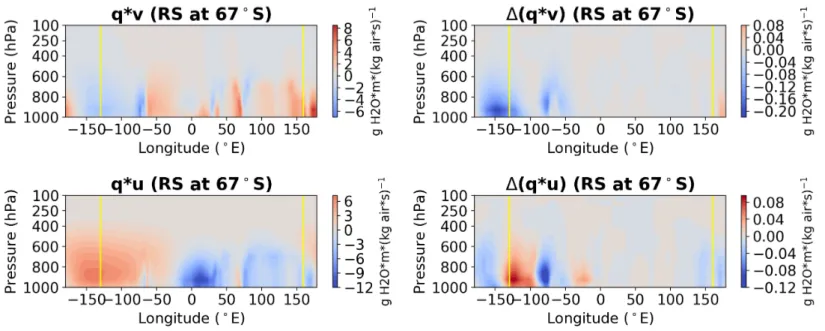
Figures 3.8, 3.9, and 3.10 show the vertical structures of moisture fluxes averaged over cases with low SIC within each specific region. The zonal and meridional moisture fluxes at a given point were calculated as the product of specific humidity q and the wind components u and v, respectively. Each latitudinal section was chosen to be at a representative center of the region’s moisture flux anomaly.

Figure 3.8: Vertical profiles of mean zonal and meridional moisture transport (q · u and q · v, respectively) averaged over cases in the 10th _{percentile monthly mean SIC anomalies}

and the average differences from the overall mean, ∆(q · u) and ∆(q · v), in the Ross Sea (RS) region (yellow lines indicate boundaries: west of 130° W, east of 160° E) across 67° S. Note that colorbars are scaled differently for each plot.

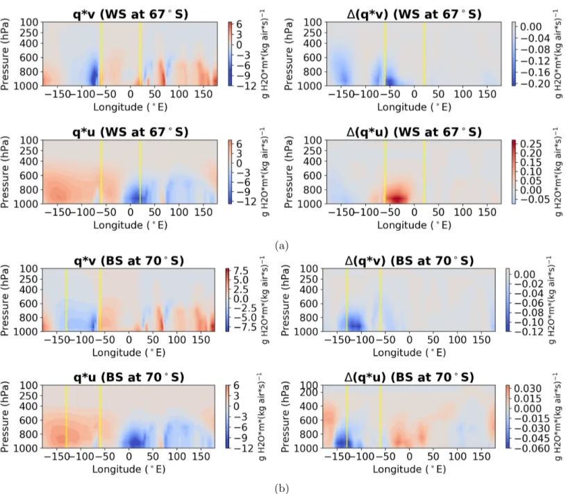
(a)

(b)

Figure 3.9: Vertical profiles of mean zonal and meridional moisture transport (q·u and q·v, respectively) averaged over cases in the 10th _{percentile monthly mean SIC anomalies and}

the average differences from the overall mean, ∆(q · u) and ∆(q · v), in (a) the Amundsen and Bellingshausen Seas (BS) region (west of 60° E, east of 130° W) across 70° S and (b) the Weddell Sea (WS) region (west of 20° E, east of 60° W) across 67° S. Yellow vertical lines indicate the boundaries of the region. Note that the colorbars are scaled differently for each plot.

(a)

(b)

Figure 3.10: Vertical profiles of mean zonal and meridional moisture transport (q · u and q · v, respectively) averaged over cases in the 10th _{percentile monthly mean SIC anomalies}

and the average differences from the overall mean, ∆(q · u) and ∆(q · v), in (a) the Indian Ocean (IO) region (west of 20° E and east of 90° E) across 65° S and (b) the Pacific Ocean (PO) region (west of 160° W and east of 90° W) across 64° S. Yellow vertical lines indicate the boundaries of the region. Note that colorbars are scaled differently for each plot.

The Ross Sea region’s profile shown in Figure 3.8 shows a high eastward moisture transport at its 130° W border, in line with the zonal moisture transport discussed in relation to circulation patterns seen in Figure 3.6. The poleward moisture flux that tested as significant (in Figure 3.3) can also be seen near 130° W. In Figure 3.9(a), a poleward moisture flux with a southward deflection from the mean moisture flux can be seen in the Amundsen and Bellingshausen Seas, near to where the stationary moisture influx at the Antarctic Peninsula exists – as one of the primary sources of heat in the Antarctic (Oshima et al., 2004), it is expected that more warm, moist air at this point can lead to an overall decrease in Antarctic SIC. Eastward winds at its western boundary (around 155° W) are weaker than normal, which may serve to decrease zonal moisture transport out of this region. For the Weddell Sea, in Figure 3.9(b), the significant meridional section of anomalous moisture flux seen in Figure 3.3 is clear in the region from 40-60° W, but the total absolute moisture transport is not southward. Instead, greater eastward transport is present to the west from the neighboring Bellingshausen and Amundsen Seas, indicating that the source of moisture during months with low SIC is to the west. With Figure 3.10(a), the low sea ice concentration in the Indian Ocean section becomes more difficult to explain with moisture flux. Moisture fluxes are both northward and southward in this region, with no particular anomalies, as expected from the significance test results in Figure 3.3. The zonal transport is also very near the mean state with little anomaly. The Pacific Ocean section’s vertical profile along 90° W shown in Figure 3.10(b) has a positive absolute moisture flux at the surface along this latitude during states of low SIC, although the difference from mean is negative; in this region, northward flow typically circulates air out of the region (as seen in Figure 3.5), so that a decreased northward transport may be causing an accumulation of moisture in the region. However, it is clear from the significance tests in Figure 3.3 that polar moisture flux variation does coincide with cases of low sea ice concentration; in three of the five sections, a significant poleward anomaly can be seen within the region of interest, while in four of the five sections, a significant poleward anomaly can be seen elsewhere in the Antarctic polar region.

Figures 3.11, 3.12, and 3.13 include vertical profiles of specific humidity and tem-peratures along with their differences from overall mean values averaged over the low SIC composites for each region.

(a)

(b)

Figure 3.11: Vertical profiles of specific humidity and temperature averaged for months with anomalously low (10th percentile) monthly mean SIC composite distributions as well as their differences from the overall mean for (a) the Ross Sea (RS) region (west of 130° W, east of 160° E) across 67° S and (b) the Amundsen and Bellingshausen Seas (BS) region (west of 60° E, east of 130° W) across 70° S. Yellow vertical lines indicate the boundaries of the region. Note that colorbars are scaled differently for each plot.

(a)

(b)

Figure 3.12: Vertical profiles of specific humidity and temperature averaged for months with anomalously low (10th percentile) monthly mean SIC composite distributions as well as their differences from the overall mean for (a) the Weddell Sea (WS) region (west of 20° E, east of 60° W) across 67° S and (b) the Indian Ocean (IO) region (west of 20° E and east of 90° E) across 65° S. Yellow vertical lines indicate the boundaries of the region. Note that colorbars are scaled differently for each plot.

Figure 3.13: Vertical profiles of specific humidity and temperature averaged for months with anomalously low (10th _{percentile) monthly mean SIC composite distributions as well}

as their differences from the overall mean for the Pacific Ocean (PO) region (west of 160° W and east of 90° W) across 64° S. Yellow vertical lines indicate the boundaries of the region. Note that colorbars are scaled differently for each plot.

Anomalously high specific humidities are often found with a nearly identical struc-ture of positive temperastruc-ture anomalies. The results shown in Figures 3.8-3.10 and in Figures 3.11-3.12 show that the greatest amount of moisture transport is near the sur-face. In Figure 3.11(a), the Ross Sea section contains another clear temperature anomaly of up to + 1.8 K at 150° W, and the temperatures at its eastern boundary are the highest along this latitude. Specific humidity is also high at this boundary, ∼ 0.25 g kg−1 higher than the mean humidity at the 1000 hPa level at 150° W. In (b), the Amundsen and Bellingshausen Seas see temperature anomalies in higher pressure levels in the composite of cases with low sea ice concentration. The specific humidity anomaly is located precisely in the region of interest. In Figure 3.12(a), the Weddell Sea region includes yet another positive average specific humidity anomaly for the local low SIC cases. The average tem-perature within the Weddell Sea section is up to 2.5 K higher than its mean. The Indian Ocean region’s profile plotted in (b) shows a different behavior in association with the cases of anomalously low SIC; the temperature is equal to or even lower than the mean for its sector, and the specific humidity is also up to - 0.22 g kg−1 lower than the mean. The Pacific Ocean section, in Figure 3.13, exhibits clear specific humidity anomalies in the region of interest, as well as a temperature anomaly of up to 1.9 K at the 1000 hPa

Section 4

Discussion and Conclusions

4.1

Discussion

January, February and March (but most particularly February) are underrepresented in the distribution of the 10th monthly mean SIC anomalies in all regions. The Antarc-tic summer historically sees a total retreat of sea ice during the summer (Cavalieri and Parkinson, 2008), hence the low number of cases with anomalously low sea ice concen-tration during these months – if the average is close to zero sea ice then there can only be little or no negative anomaly. It can also be seen that there are a larger number of cases in the SH springtime (September, October, November) with anomalously low sea ice concentration; the months where sea ice is present and undergoing a dynamic change will be sensitive to variations in conditions and larger anomalies will result. Drawing conclusions about the conditions in the time period leading up to anomalously low SIC would require a different approach and methodology, so the focus in this study remains on the monthly mean values for atmospheric conditions concurrent to the cases of low monthly mean SIC.

What is noticeable in the fields of VINMF anomalies is the dipole behavior; merid-ional sections of moisture anomalies come in pairs of nearly neighboring positive and negative anomalies, reaching far into the continent. In the cases of low SIC in the Wed-dell Sea, Ross Sea, and Pacific Ocean, there is a meridional section of negative VINMF anomalies, i.e. more moisture flowing southward towards the pole than the mean field. The cases of low SIC in the Indian Ocean actually exhibit the opposite, a higher north-ward moisture flux than the mean that tests as significantly different. There is, however, a

clearly significantly strong poleward moisture flux opposite in the Ross Sea section flanked by two positive anomalies in these cases. Also evident in the VINMF anomaly fields is the fact that significant anomalies can often be found particularly in the western part of the continent and the Antarctic peninsula (in the same positions during the low mean SIC distributions for the Weddell Sea, Ross Sea, and Indian Ocean sections), which is where most of the local warming has occurred in recent years, from observations carried out since 1957 (Bromwich et al., 2013). In addition, due to the general warming in the western part of the continent, local decreases in sea ice concentration have been observed (Stam-merjohn et al., 2012) and the mean sea ice concentrations in these regions are drawn down by the decrease; this is most evident in the Amundsen and Bellingshausen Seas. The lack of moisture flux anomalies within the Bellingshausen and Amundsen Seas region during cases of low mean SIC may be due to a stronger connection between increased cyclone strength in the Ross Sea region and low SIC, as well as warm air transport in the Bellingshausen and Amundsen Seas region (Fogt et al., 2011).

It is possible that sea ice conditions in many of the regions are more strongly linked to the Southern Annular Mode (SAM) – this connection is a relatively recent subject of research and requires further study, but it is probable that the primary reason for variability in circulation in the southern polar region is the SAM, as well as the concurrent phase of the El Ni˜no-Southern Oscillation (ENSO) (Fogt and Bromwich, 2006). Recent changes (since the 1980s) in the seasonal cycle in Antarctic sea ice have been linked to the phase of the SAM – a negative phase of the SAM leads to more favorable conditions for sea ice formation (cool winds that lead to divergence in the sea ice, transporting it away) in the Amundsen and Bellingshausen Seas region, but to less favorable conditions in the Ross Sea region (warm winds transporting sea ice onto the coast). In a positive oscillation, the Antarctic Circumpolar Current comes closer to the Antarctic continent and intensifies, as do the westerly winds – these conditions lead to the upwelling of warm deep water (Anderson et al., 2009), accelerating melt in the ice sheet (Greene et al., 2017). These circulation patterns are caused by high pressure at high southern latitudes and low pressure on the Antarctic continent and coast, with a distinctive tripole pattern of high pressure centers surrounding the continent, leading to a steep pressure gradient. The conditions for a positive oscillation can be seen clearly in the cases of low sea ice for the Pacific Ocean and Weddell Sea regions in Figure 3.5(b) and 3.7(a), respectively, linking

the conditions described in Greene et al. (2017) to anomalously low sea ice concentration. The cases of low SIC in the Bellingshausen and Amundsen Seas region, as well as those of the Indian Ocean, display the typical conditions for a negative oscillation (reversed geopotential height anomalies; higher pressure over the Antarctic continent). This does not agree with Fogt and Bromwich (2006), but the seasons in which the low monthly mean SIC cases used for this study occur have not been separated; in order to make a statement on whether these results agree, the mean geopotential height anomalies for the SH fall must be analyzed in order to see what the SAM phase (and its strength) is during the seasonal sea ice formation. A weak signal of the negative phase for the SAM is seen in the mean geopotential height anomalies in the Ross Sea over months with low mean SIC, which aligns with less favorable conditions described in Fogt and Bromwich (2006). As well as disagreeing with the SAM-driver hypothesis, the Indian Ocean region’s states of low SIC do not seem to align with the moisture-driven hypothesis. Another possible explanation for low sea ice concentration in this region is a dominance of ocean transport (there are known northward outflows in oceanic transport of sea ice in this region as outlined in Heil and Allison 1999).

The geopotential height and wind anomaly fields during months with anomalously low mean SIC may explain how moisture is transported easily into the Ross Sea region. In the case of the Amundsen/Bellingshausen Seas section, there is a positive geopotential height anomaly directly on the coast, which may also brake incoming wind along the moisture corridor that exists off of the Peninsula. The geopotential anomaly field in the Weddell Sea is very similar to that of the tripole pattern of the SAM; its negative can be seen in the Ross and Bellingshausen sea cases. The Weddell Sea is seeing increased zonal transport (corroborated in Figure 3.9(a), and in line with prior studies such as Tiet¨av¨ainen and Vihma 2008) from near the Antarctic Peninsula during these cases, along the coast and eastward. A similar pattern is evident in the Pacific Ocean during the low sea ice concentration cases.

4.2

Limitations

It would have been greatly useful to ensure that all variables investigated in this study (specific humidity, temperature, geopotential height, wind components, and the moisture

transport variables u times q and v times q) were tested for significance using the Student’s t-test, just as VINMF was tested in this study, in order to understand where the differences from the mean are truly significant and to strengthen comments made on profiles of humidity and temperature as well as fields of geopotential height and winds. In this way, the comments made upon negative/positive average anomalies during months of low SIC could become robust arguments about how the atmospheric circulation, moisture and thermodynamic variables differ from the overall mean climate of the region. What would also improve and strengthen the analysis of the conditions presented in this study would be a more distinct separation between the months in which the anomalously low SIC occurs for investigating atmospheric variables during specific seasons; while comments made on the state of average circulation anomalies are backed by evidence that there are significant differences in atmospheric circulation during months with anomalously low SIC, they do not have the capacity to be applied specifically to seasonal change in the sea ice region. A more detailed idea of how atmospheric circulation in the Antarctic polar region is linked to lower SIC could be achieved by looking at the anomalies in circulation averaged over separated seasons, so that one could investigate how the circulation affects sea ice formation (during SH autumn and winter), destruction (the retreat during SH spring), and persistence (how long sea ice remains during SH spring and summer) separately. Further work on this could give better understanding of the specific sensitivities of each region to moisture fluxes during given seasons.

Another limitation of the presented study is the lack of alternative datasets, in-situ observations, and number of observations with which to validate and check the results against. The sea ice concentration dataset used for this study is quite unique and has few peers – especially given its large coverage in both spatial scale and time. For both sea ice concentration and all atmospheric circulation parameters, there is a general lack of in-situ observations in the Antarctic polar region due to the cost of sending research equipment and personnel there. The accuracy of sea ice concentration datasets could otherwise be improved by validating against in-situ measurements in order to better tune algorithms used in calculating sea ice concentrations, and to better understand where contributions to error occur in the measurements as well as the retrieval process from raw satellite radiometry data. For atmospheric dynamics, a greater amount of in-situ observations are also needed for increasing the accuracy of reanalysis datasets, because of the way that

reanalysis is performed: extrapolated values from forecast models must be checked against and adjusted towards observational data. Researching moisture in the Antarctic region in detail presents particular difficulties, because of the disagreement between reanalysis and observation in clouds (Lawson and Gettelman, 2014) and precipitation (Palerme et al., 2017) within this region. This will have to be addressed if studies involving reanalysis datasets are carried out with a focus on the qualities of the moisture, precipitation, and clouds within the Antarctic polar region. A larger sample size and geographic coverage in Antarctica would help in strengthening the reliability of ERA and many other reanalysis databases. More samples (longer coverage) in the sea ice concentration datasets would lead to stronger statistical testing – carrying out the same procedure with testing moisture and atmospheric variables from the lowest percentile of SIC with a larger population size of both and having similar results at a higher confidence level would lead to more convincing results.

4.3

Societal Implications

In the face of a globally warming climate, it is of utmost importance that we are able to make predictions about how the climate will change in the coming years in order to prepare and make informed policy decisions. The importance of issuing mitigation poli-cies if accelerated, long-term consequences (social, ecological, and economic) from climate responses are to be curtailed is quickly growing. Our primary method of doing so is currently through the use of general circulation models (GCMs), which inform goals and benchmarks for limiting sources of greenhouse gases. However, in their present state, GCMs do not completely agree with each other and have a large spread of predictions and uncertainties (Knutti and Sedlacek, 2012). This spread and disagreement is per-haps the greatest weakness in climatological research today, a weakness that is frequently politicized and used to work against climate mitigation policies. From this study, it is evident from the lack of detailed knowledge – as well as the lack of a way to validate studies using alternative datasets and in-situ measurements – of the relationship between circulation patterns in the Antarctic sea ice region and sea ice formation/destruction that further research is needed to improve our understanding of climate in sea ice regions. GCMs are known to do a poor job in accurately simulating sea ice concentration in the

Antarctic region (Massom and Stammerjohn, 2010), but there is a general consensus that the Antarctic sea ice region will see significant losses during this century (Pachauri et al., 2014), as much as 33% in wintertime extent by the year 2100 (Bracegirdle et al., 2008). The continent itself is projected to see a warming at the surface of 0.34° C per decade (±0.10° C); on top of this, the general circulation patterns are projected to see a change with an increased frequency of positive SAM phases, bringing westerly winds nearer Antarctica and altering the conditions in which sea ice is formed, transported, and destroyed. interact with each other. A differential in planetary characteristics (albedo, temperature, pressure, etc.) between the polar regions and lower latitudes is a key driver of dynamics in climate; a weakening of this characteristic (such as decreasing the albedo of the polar region with sea ice melt) would perturb global climate in ways not seen in human history. Seeking further understanding of the interactions between cryosphere, ocean, and atmosphere in the Antarctic polar region is crucial in improving accuracy of GCMs and thus how we prepare, decide on policies, and act on them.

There is also a clear connection between climate and circulation patterns in the Antarctic polar region and those in other parts of the southern hemisphere (such as Australia and South America), during phases of the SAM; what meteorological processes occur within the Antarctic polar region that affect the strength of this oscillation has an effect on climate in populated regions as well. If the pressure gradient between the Antarctic continent and the Southern Ocean is made steeper (weaker) by sea ice dynamics in the region, then the SAM phase is strengthened (weakened). During negative phases, storms, precipitation and low pressure systems occur more often in middle latitudes; during the positive phase, the westerlies being drawn closer to the Antarctic continent leads to dryer conditions in mid-latitudes, affecting both Australia (Raut et al., 2014) (the drought in Australia that lasted from 1997 until 2010 is thought to be related to the SAM, and the frequency of droughts related to the SAM is predicted to increase according to Cai et al. 2011) and South America (Gillett et al., 2006). The positive phase of the SAM is also correlated to significantly increased incidence of wildfire events across the southern hemisphere due to these warmer, dryer conditions (Holz et al., 2017). Greater understanding of the interaction between sea ice concentration in the Antarctic that affects meteorological patterns in lower, more inhabited latitudes would benefit those living in areas such as Australia and Central and South America in terms of preparation

and advisement by meteorological agencies for shifts in precipitation, temperature, and storm patterns.

4.4

Conclusions

There are clear differences in circulation patterns between the cases of the largest negative sea ice concentration anomalies and the overall mean flow. To test the hypothesis that anomalously high moisture influxes are connected with anomalously low sea ice concentra-tion, the poleward moisture fluxes below the 10th _{percentile of mean sea ice concentration}

anomalies in five regions of the Antarctic were tested against the total population of meridional moisture fluxes. Plotting the de-seasonalized anomalies in moisture fluxes along with contours of areas where anomalies are significantly different at the 95% con-fidence level reveals clear signals of high poleward moisture fluxes during months with low mean sea ice concentration. The Ross Sea, Weddell Sea, and Pacific Ocean regions shows clearly significant anomalies in the direction of the pole, indicating that moisture is brought closer to the Antarctic continent and to the sea ice production zone during months with low sea ice concentration. In the case of low SIC in the Bellingshausen and Amundsen Seas region, there is no clear moisture flux anomaly within the section of in-terest but rather a northward anomaly (away from the pole) in the Ross Sea and Pacific Ocean region.

Upon inspecting vertical structures of monthly mean moisture and temperature, a specific humidity “pocket” higher than the overall mean is seen directly in the regions in which the low monthly mean SIC occurs, indicating that the fluxes may be accumulating moisture within their bounds. Furthermore, the differences in temperature from the overall mean show an increase in temperatures in the same shape, bounds, and pressure levels as the specific humidity “pockets” in conjunction with low SIC. The region in which the distribution of low monthly mean SIC occurs often exhibits the highest temperatures at that latitude. This supports the hypothesis that there is a clear link between the heat transported by high influxes of water vapor and the ability to accelerate the melting of sea ice. Although the Antarctic polar region sees relatively small variations in circulation patterns, the differences in circulation during the composite distributions of months with low mean SIC are clear. Geopotential height anomalies introducing circulation patterns

above the background mean circulation change the way that moisture is transported, often increasing poleward moisture transport (as is the case in the Ross Sea, Pacific Ocean, and Weddell Sea during months with low mean SIC), or affecting zonal transport, such as in the case of low SIC in the Bellingshausen and Amundsen Seas.

In recent years, evidence has been presented that ties the phase of the Southern Annular Mode as well as that of the El Ni˜no - Southern Oscillation phase together in determining conditions that affect sea ice formation and destruction (Clem et al., 2016). Fields of mean geopotential height anomalies during the cases of low SIC in the Belling-shausen and Amundsen Seas, Weddell Sea, Pacific Ocean and Indian Ocean regions show signs of strong connection to the SAM phase; there is a clear signal of the positive phase of the SAM in the Weddell Sea and Pacific Ocean sections during the distribution of months with anomalously low monthly mean SIC, while in the Indian Ocean and Bellingshausen and Amundsen Seas sections, the negative phase is seen to coincide with cases of low SIC. While far-reaching effects of circulation in the mid-latitudes or coastal upwelling in the ocean increasing melt underneath sea ice may be the cause of the weak signal in poleward moisture flux anomalies in the Indian Ocean region during months with low mean SIC, it is hard to find an alternative explanation within the results of this study for the fields investigated that is supported by other evidence.

4.5

Suggestions for Further Study

The conditions surrounding anomalously low SIC in the Antarctic are complex; there are numerous methods that would be useful in investigating the causes for sea ice anomalies in the southern polar region that were not employed in this study. This study made use of only a few of the fields essential to gaining an understanding of the circulation patterns in the Antarctic, and on a general, polar region-wide scale. It is clear that regional differences are great, and investigating states of low sea ice concentration on a more local scale is essential for a clear picture of interactions between sea ice and the atmosphere in the Antarctic polar region. To this end, a few methods for extending the study that can be used for greater understanding of the links between circulation, moisture and sea ice concentration will be discussed.

a region as well as the fluxes in and out for a quantification of total moisture parameters within a region, and regression analysis between these and sea ice. The total moisture content of the air mass within a sea ice region can easily be calculated using reanalysis tools, and the vertically integrated fluxes along northern, eastern and western boundaries would give fluxes and rates of accumulation (for atmospheric transport – evaporation and precipitation can be easily included to complete the budgeting). Each of these variables allow for a single quantity that can be tested for correlation with sea ice extent or concen-tration, as well as the rate of retreat or growth. A similar approach to Johansson et al. (2017) can be used with total moisture influx into the region along important boundaries, such as through the “corridor” of inflow near the Antarctic Peninsula shown in Oshima et al. (2004), and comparing to the total sea ice extent. These correlations may then be related to radiative forcing parameters previously calculated for changes in sea ice as well. This statistical method would strengthen the analyses carried out in this study and test its conclusions for an idea of just how strongly correlated these few parameters are.

Joining the study with an overview of the the radiative effects of the higher-than-average humidities, moisture fluxes, and changes in sea ice concentration can also give a more complete understanding of how strong the effects of each of these parameters are. For this, a vertical energy balance model could be of use. The albedo changes due to sea ice concentration, the increased potential for evaporation as sea ice melts, the effects of moisture as a greenhouse gas, cloud processes, and upper layer ocean processes would be key inputs for a study of the radiative balance of the sea ice region. For the sake of the experiment, a closed system with control variables could be employed to force parameters such as moisture flux and accumulation and study the subsequent effects of isolated variables. Historical values and records of moisture influxes over a region (such as budgets described in the previous paragraph) could be fed into the model and tested against data from observations. An idea of the strength of each variable’s effects in the region as well as the feedback loops involved could also be gained in this way. It may also be a way to investigate the magnitude of the effect of oceanographic variables on southern sea ice where atmospheric conditions are not dominating its formation or destruction.

Further analysis focused on the phases of both the Southern Annular Mode and the El Ni˜no - Southern Oscillation in relation to sea ice concentration and atmospheric circulation patterns is justified, and interest in this has been expressed in recent research

(Fogt and Bromwich, 2006)(Greene et al., 2017)(Clem et al., 2016). A similar region-focused approach such as in this study should be employed as the effects of the SAM on each region differs with the mean patterns that it brings, as well as any local upwelling that may occur (Anderson et al., 2009). The phase numbers associated with the SAM and the ENSO (as well as the combinations thereof) could also be tested against the sea ice concentration and extent anomalies in each region for an understanding of where the greatest connection to the state of the sea ice lies. Understanding in which season they occur is also crucial.

It would be useful to include work focusing on the cloud effects of water vapor influxes. A weakness of the approach in this study is that it does not take into account any differentiation between cloud cover and any unsaturated humidity – instead, only integrated column moisture contents as well as specific humidities were considered. There is a great qualitative difference in the presence of moisture’s local effects between water vapor and cloud formation, and a real distinction between clear-sky and cloudy conditions with separate analyses would be necessary to understand exactly how each interacts with the sea ice region. While one aim of this study was to understand links between the presence of moisture with states of low sea ice concentration, it would not be possible to draw complete conclusions of the nature of these interactions solely with the methods employed here. As well, the phases of the water within the atmosphere determine their effects; the portions of liquid and ice water play a role in the radiative effects of clouds in the Antarctic (McCoy et al., 2015), which is consistently misrepresented in GCMs (Lawson and Gettelman, 2014). Further work on feedbacks between sea ice, moisture, and cloud formation specifically in the southern polar region could help reduce these difficulties in modeling global climate, which is of utmost importance in policy planning based on realistic predictions of future climate. Difficulties may come about due to the uncertainty of observational data retrieved for clouds in the Antarctic and Arctic regions, however (Bromwich et al., 2012).

Lastly, a model comparison that would seek to investigate whether the moisture fluxes in the Antarctic coincide with reductions in sea ice in an ensemble of GCMs, and whether the associated circulation patterns agree with observations, would help give un-derstanding in how accurately the climate variables investigated in this study are modeled and potentially pinpoint another source of uncertainty. Individual models may be

com-pared in order to understand where agreements and disagreements lie in how well sea ice dynamics as well as the local atmospheric parameters that affect them are perform-ing. Analyzing the effects of the phases of the SAM and ENSO on SIC would be a test of complex interactions and teleconnections in global climate. If there is disagree-ment between historical observations and how the phases align with behavior in SIC and formation/destruction of sea ice in the models, then there would be a few important questions to be posed: why do models under- or overrepresent sea ice during distinct phases of circulation patterns, and how does this create uncertainty? Where is heat and moisture being transported during modes of circulation within the models, and do they agree with observations? Does the sea ice in the Antarctic seem to vary on the decadal scale in the models as it does in observations, and does this align with the decadal vari-ability of the SAM as postulated in Fogt and Bromwich (2006)? Seeking answers to these pertinent questions would undoubtedly give insights to weaknesses in GCMs and lead to improvements on predictions of future climate.