LDD: Learned Detector and Descriptor of Points for Visual Odometry

IN

DEGREE PROJECT COMPUTER SCIENCE AND ENGINEERING, SECOND CYCLE, 30 CREDITS

,

STOCKHOLM SWEDEN 2018

LDD: Learned Detector and

Descriptor of Points for Visual

Odometry

JEVGENIJA AKSJONOVA

KTH ROYAL INSTITUTE OF TECHNOLOGY

LDD: Learned Detector and

Descriptor of Points for Visual

Odometry

JEVGENIJA AKSJONOVA

Master of Science in Machine Learning Supervisor: Josephine Sullivan

Examiner: Patric Jensfelt E-mail: jevaks@kth.se

School of Electrical Engineering and Computer Science Date: August 24, 2018

iii

Abstract

Simultaneous localization and mapping is an important problem in robotics that can be solved using visual odometry – the process of es-timating ego-motion from subsequent camera images. In turn, visual odometry systems rely on point matching between different frames. This work presents a novel method for matching key-points by apply-ing neural networks to point detection and description. Traditionally, point detectors are used in order to select good key-points (like cor-ners) and then these key-points are matched using features extracted with descriptors. However, in this work a descriptor is trained to match points densely and then a detector is trained to predict, which points are more likely to be matched with the descriptor. This information is further used for selection of good key-points. The results of this project show that this approach can lead to more accurate results compared to model-based methods.

iv

Sammanfattning

Samtidig lokalisering och kartläggning är ett viktigt problem inom ro-botik som kan lösas med hjälp av visuell odometri – processen att upp-skatta självrörelse från efterföljande kamerabilder. Visuella odometri-system förlitar sig i sin tur på punktmatchningar mellan olika bildru-tor. Detta arbete presenterar en ny metod för matchning av nyckel-punkter genom att applicera neurala nätverk för detektion av punk-ter och deskriptorer. Traditionellt sett används punktdetektorer för att välja ut bra nyckelpunkter (som hörn) och sedan används dessa nyc-kelpunkter för att matcha särdrag. I detta arbete tränas istället en de-skriptor att matcha punkterna. Sedan tränas en detektor till att förutspå vilka punker som är mest troliga att matchas korrekt med deskriptorn. Denna information används sedan för att välja ut bra nyckelpunkter. Resultatet av projektet visar att det kan leda till mer precisa resultat jämfört med andra modellbaserade metoder.

Contents

1.2 Ethical considerations and societal impact . . . 6

2 Background 7 2.1 Deep Convolution Neural Networks . . . 7

2.1.1 Training Neural Networks . . . 8

2.1.2 Convolutional layer . . . 9 2.1.3 Batch Normalization . . . 10 2.1.4 ResNets . . . 10 2.2 Baseline Methods . . . 11 2.2.1 SIFT . . . 11 2.2.2 DAISY . . . 11 3 Methods 13 3.1 Data . . . 13 3.1.1 KITTI . . . 13 3.1.2 FlyingThings . . . 14 3.1.3 Augmentation . . . 14 3.1.4 Evaluation . . . 14

3.2 Learning the Descriptor . . . 15

3.2.1 Training . . . 17

3.3 Learning the Detector . . . 18

3.3.1 Construction of the ground truth data . . . 18

3.4 Point selection . . . 20

vi CONTENTS

3.5 Implementation details . . . 22

4 Results 23

4.1 Descriptor . . . 23 4.2 Detector . . . 24 4.3 Combining the Descriptor and Detector . . . 26

5 Discussion and Conclusions 31

5.1 Discussion . . . 31 5.1.1 Drawbacks and future work . . . 31 5.2 Conclusions . . . 32

Chapter 1

Introduction

Simultaneous Localization and Mapping (SLAM) is an important prob-lem in robotics. The objective is to simultaneously estimate ego-motion and construct a map of the environment. In visual SLAM information obtained from the camera is used to solve this problem. This involves estimating ego-motion from the subsequent camera images – the pro-cess called visual odometry.

There are different ways to perform visual odometry. For instance, Bundle Adjustment (BA) can be used to jointly estimate the positions of the camera and the positions of points in space, given that these points were captured by the camera from different view-points [16], [24]. This is illustrated in figure 1.1. Methods that use BA are usu-ally called sparse feature-based methods. One of the state-of-the-art feature-based systems is ORB-SLAM [27]. An alternative approach to

Figure 1.1: BA setup: points are projected into several image planes, [24].

2 CHAPTER 1. INTRODUCTION

BA is to estimate the displacement of the camera by aligning images so that the photometric error is minimized. This approach can be used to obtain a dense or semi-dense map of the environment, for instance, as in LSD-SLAM [11]. However, sparse feature-based methods are mostly used in practice.

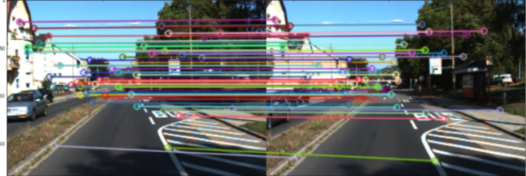
As we can see in figure 1.1, in order to use BA it is necessary to find points in the images that correspond to the same points in space. In other words, BA relies on point matching between different frames. There are different feature extraction methods that can be used to de-tect and reliably match key-points. For instance, the ORB-SLAM [27] makes use of the ORB features [31] in all subtasks, such as, tracking, mapping, relocalization and loop closing. Some methods propose al-gorithms for both detection and description of key-points, for instance, SIFT [25], SURF [3] and ORB [31]. While others, like Harris Corner De-tector [15] and FAST [30], focus on detection of points that would be sta-ble and repeatasta-ble across different frames. An example of key-points detected and matched with SIFT is illustrated in figure 1.2.

Figure 1.2: Example of key-points detected and matched with SIFT. Artificial neural networks is a class of models used in Machine Learn-ing, which gained an increased popularity over the last decade. Deep Convolutional Neural Networks have been used to achieve state-of-the-art results in computer vision tasks, for instance, image classification [22], object detection [29] and semantics segmentation [23]. Despite the great potential of deep learning features to define and match key-points, model-based local descriptors still dominate the field.

Recently, there have been many attempts to create learned local de-scriptors using neural networks. For instance, DeepCompare [43],

CHAPTER 1. INTRODUCTION 3

compare small image patches and, as indicated in a comparative survey [33], they are not bound to a particular choice of detector. Therefore, they are often used in combination with hand-crafted point detectors. More recent works have proposed to extract features densely for all points. For instance, [6] proposed the Universal Correspondence Network (UCN) for learning the feature space using dense correspon-dences, such as disparities in stereo images. The resulting model pro-duced a dense feature map for each image and then points could be matched between different images with the Nearest Neighbor algo-rithm. Furthermore, [8] and [37] combined dense feature extraction with score prediction, so that a score value can be used to decide if the point should be selected as a key-point or not. [8] aimed to predict “cor-nerness” of points by pre-training the detector on a synthetic dataset with geometric figures, whereas [37] used Harris corners to provide the ground truth data for the detector. These works are still somehow based on model based methods even though they push the learned detector to generalize over the model-based ground truth during the training.

This Master’s thesis poses a question: in the case of dense feature extraction, is it possible to create a detector by simply predicting which points are more likely to be matched? This work tries to answer this question by constructing a new type of ground truth data for the de-tector: points are divided into good and bad depending whether they are matched between images in all-to-all matching scenario or not. To do this, we first train a descriptor that we call LDesc, which creates a dense feature map for each image. Then we construct the ground truth data and train a detector that we call LDet to discriminate between 2 classes: “matched” or “not matched”. Deep Neural Networks are used for both of these tasks.

In the process we have discovered that scores predicted by the de-tector are not repeatable enough for selecting points with a simple non-maximum suppression and performing sparse matching on the selected points. Therefore a semi-dense matching procedure is proposed for the evaluation. We call the combined method LDD (Learned Detec-tor and DescripDetec-tor) and evaluate it on augmented stereo images from synthetic FlyingThings dataset [28] and image pairs from KITTI Stereo and KITTI Optical Flow [12], [26]. The results show that LDD leads to more accurate point matching than SIFT in our experiments.

4 CHAPTER 1. INTRODUCTION

the research problem and describes related work. The second section briefly describes the basics of deep learning and methods used as a baseline. Third section introduces the LDD method and, finally, fourth and fifth sections present and discuss the results.

1.1

Related work

The idea of predicting which points are likely to be matched is not abso-lutely new. For instance, [17] tried to predict which key-points survive through the matching process of the traditional Structure-from-Motion pipeline. The authors of [32] pointed out that many of the proposed methods for learning detectors utilize model-based features for train-ing and this might be a huge limitation. They proposed an unsuper-vised learning approach: first, the model, called Quad-Networks, was trained to produce a consistent ranking of points, then key-points were defined as the top/bottom quantiles of the ranking.

1.1.1

LIFT

In [40], the authors focused on the repeatability of key-point detection under drastic changes in conditions. The detector called TILDE was trained using images of outdoor scenes captured with a static camera. Good key-points were identified using SIFT features [25] and used to create the ground truth data. Typically, SIFT was able to detect key-points only under good conditions. However, as a result of the training process, the detector had to learn to generalize over SIFT and detect the key-points independent of weather or lighting. The evaluation of the method provided the evidence that this was the case.

Later, [42] was the first work to propose a complete trainable pipeline composed of three components, the detector, orientation estimator and descriptor. Architectures of different parts were based on [40], [41] and [34], respectively. The components were trained sequentially. First, the descriptor was trained independently and, in the end, the detector was trained keeping the other two components fixed. The results showed that optimizing different components jointly is essential for achieving an optimal performance of the full pipeline. Notably, this work also exploited the idea of learning to detect points, which are easy to match with a given descriptor.

CHAPTER 1. INTRODUCTION 5

1.1.2 SuperPoint

Furthermore, [9] proposed a CNN for corner detection, called

Magic-Point. In order to train the network, they generated a synthetic dataset,

which consisted of images with simple geometric shapes with known ground truth corner locations. In [8] the MagicPoint detector was uni-fied with the UCN descriptor [6]. The resulting model was trained in a self-supervised manner: first, the detector was pre-trained on a synthetic dataset from [9], then iterative fine-tuning of the network was performed, by providing warped real-world images as the train-ing examples and ustrain-ing key-points detected in the previous steps as the ground truth data. This was done to improve generalization abilities of the model.

1.1.3 GCN

Another work similar to ours is [37]. In this works the authors defined Geometric Correspondence Network (GCN) to learn to detect and de-scribe key-points simultaneously. They used the ResNet architecture to extract features and a recurrent bi-directional structure on top of the features to produce a key-point mask. Harris key-point detector was used to create the ground truth data for training. Similarly as in [40], a key-point detected in one image might not be detected in an-other related image, thus the network had to learn to generalize over the model-based detector. In addition, the recurrent structure exploits temporal information and should enforce repeatability of key-points across different frames.

1.1.4 Dense matching

Point matching is a crucial subproblem in many different tasks. For in-stance, the task of depth estimation involves matching corresponding pixels in two images of the same scene. Images obtained with a stereo camera usually are rectified (aligned with a common plane), therefore, the displacement of points is possible only along the horizontal direc-tion. In this case the displacement is called disparity. Inspiration for this project came from a work on dense disparity estimation [21].

In this work a matching-cost-volume was formed by concatenat-ing features extracted with a Siamese network over all possible dis-parity values. Then another relatively deep CNN was used to

out-6 CHAPTER 1. INTRODUCTION

put matching probabilities. This compound architecture (called

GC-Net) was trained to extract features and estimate matching

probabil-ities densely for all points in an image. During testing the disparity values that led to the smallest matching cost and the highest probabil-ity were identified. A large synthetic dataset FlyingThings was used to pre-train the model.

The inspiration came from the fact that probability distribution over different disparities could potentially be used to discriminate between easy to match and hard to match points. In the working process this idea has developed beyond recognition, as it has been discovered that it is easier to train a network to solve binary classification problem (“matched” or “not-matched”) than a regression problem that predicts probabilities. Nevertheless, datasets as well as network architectures used in this project are the same or very similar to [21].

1.2

Ethical considerations and societal impact

The main application of visual odometry is in robotics. Localization is a crucial subtask, which must be solved by all mobile robots. Pre-cise localization in indoor environments is necessary for help-robots in hospitals, personal assistants for disabled and elderly people, search and rescue robots as well as many other robots that could perform task that are very dangerous for people, such as work in mines.

Unfortunately, the same technologies inevitably are going to be ap-plied in the military, making the process of killing other people signif-icantly easier for parties, who posses the technology.

Apart from that, there are applications, which benefit the society in principle, however also increase risk of poverty and introduce eco-nomic segregation. For instance, while development of autonomous cars can greatly reduce costs of transportation and increase safety on the roads, it would leave many people without employment.

All in all, while there are undoubted benefits in developing tech-nologies for mobile robotics, there are certain risks that should be han-dled. Therefore the development of new technologies should proceed on par with governmental regulations.

Chapter 2

Background

This chapter describes theoretical aspects of Neural Networks neces-sary to understand the proposed solution as well as several other com-puter vision methods, which are going to be used as a baseline.

2.1 Deep Convolution Neural Networks

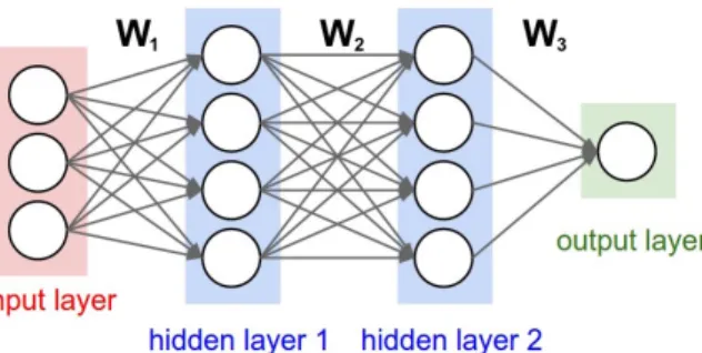
A typical architecture of a neural network consists of several layers, where each layer is a collection of computational units (neurons) of the same type. For instance, figure 2.1 shows a simple neural network with 2 hidden layers. Input and output neurons represent input and output data, while hidden neurons represent intermediate computations. Ar-rows in the image show that values computed by the previous layers are used as input for the next layer neurons.

Figure 2.1: Three-layer network architecture (with 2 fully-connected hidden layers).

A modern architecture of a Deep Neural Network can consist of

8 CHAPTER 2. BACKGROUND

layers of different types with different connection patterns. However, the most basic layer is a fully connect layer of the following form

yj = h(w0,j +

Din

∑

i=1

wi,jxi), j = 1, . . . Dout, (2.1)

where xi, i = 1..Dinis the input, yj, j = 1..Doutis the output and wi,j

are free parameters that are adjusted during the training. This layer would represent a linear function, if it was not for a non-linear activa-tion funcactiva-tion h(). For instance, popular activaactiva-tion funcactiva-tions are

ReLU (x) =max(0, x), (2.2)

sigmoid(x) = 1

1 +exp(−x). (2.3) At the last layer, it is common to apply sof tmax() activation func-tion, which ensures that the output values are in the interval [0, 1] and sum up to one. sof tmax(⃗xj) = exp xj ∑Din i=1,exp xi , j = 1 . . . Dout. (2.4)

2.1.1

Training Neural Networks

Training a neural network is minimization of a loss function with re-spect to free parameters W (weights).

If a network is used to solve a classification problem, then categor-ical cross-entropy loss is often used:

L(W ) =−

C

∑

i=1

tiln (yi(x, W )) , (2.5)

where ⃗tis a binary vector representing class assignment of x and ⃗y(x, W ) is an output of the model. In the case of regression, mean squared error (MSE) and mean absolute error (MAE) are the most common choices. In order to make the training process more efficient, predictions are usually calculated simultaneously for several data samples in a batch. Then, the total loss L(W ) is a sum of losses Lk(W ), where k is a sample

index in a batch.

The minimization problem can be solved using gradient descent op-timization. In the case of neural networks, the computation of gradi-ents is done layer by layer in a process called error back-propagation.

CHAPTER 2. BACKGROUND 9

Gradients are used to perform a parameter update with a learning rate

α:

W(t+1)= W(t)− α∇L(W(t)) (2.6) For more information on the basic neural networks please refer to [7] chapter 5.

2.1.2 Convolutional layer

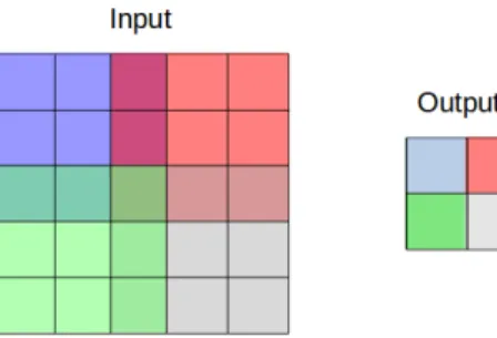
The most common neural network layer used in computer vision is a convolutional layer. As in a fully-connected layer, neurons of convolu-tional layer apply a function of the form (2.1), however, each neuron is connected only to a particular region of the input data and all neurons in a layer share the same weight parameters. Essentially, a convolu-tional layer in a neural network is very similar to a convoluconvolu-tional filter in image processing. Figure 2.2 provides the illustration. Here, a con-volutional filter of size 3× 3 is applied to an input image at 4 different locations (represented by different colors), distance between these lo-cations (2 pixels) is called a stride.

Figure 2.2: Convolutional layer with kernel size 3 and stride 2. Con-nections between input and output are represented by different (over-lapping) colors.

Convolution with stride > 1 down-samples the data. This, is used to accumulate information over large regions, while having less param-eters. However, if it is necessary to up-sample neurons back to the original dimension an operation called transposed convolution can be applied. For more information on convolutional layers please refer to [10].

10 CHAPTER 2. BACKGROUND

2.1.3

Batch Normalization

The authors of [19] have shown that applying batch normalization to hidden layers improves the speed and quality of network training. As-suming that ˆxis a D-dimensional feature vector, for each element xk, k =

1, . . . Dthe normalizing transformation has the following form:

yk=

xk− µk

σk+ ϵ × γ

k+ βk, (2.7)

where ⃗γ and ⃗β are learned parameters introduced to preserve the rep-resentational power and ϵ ensures that there is no division by zero. During the training parameters ⃗µ and ⃗σ are equal to the mean and stan-dard deviation of the features in a batch. During the inference these are moving estimates. In the case of convolutional layers ⃗µ and ⃗σ are esti-mated not only over different batches, but also over all locations in the feature map.

2.1.4

ResNets

Learning residuals is another useful technique for improving the train-ing of deep networks. Instead of learntrain-ing the desired function H(x) di-rectly, [18] proposed to learn residual function F (x) = H(x)−x. A net-work block with a residual connection is illustrated in figure 2.3. The authors of the method hypothesized that the identity function serves as a good starting point for training deep structures. This idea was supported by empirical evidence.

CHAPTER 2. BACKGROUND 11

2.2 Baseline Methods

This subsection describes two popular model-based methods, which are used for comparison in chapter 4.

2.2.1 SIFT

Scale Invariant Feature Transform (SIFT) was introduced in [25]. It is an algorithm for both key-point detection and description. The algo-rithm has three main steps. First, key-points are detected using differ-ence of Gaussians (Gaussian filters of different size are applied to the image and difference between the blurred versions is computed). This method is applied to the image at different scales and distinctive points (local extrema) in the location-scale space are identified. Next, a key-point set is refined by filtering out low-contrast key-points and edges. In order to achieve invariance to rotation, the orientation of key-points is computed based on gradient information. Finally, key-points are described by 8-bin orientation histograms computed for 16 4 × 4 re-gions around the point. Key-points are matched using nearest neigh-bor matching. In order to eliminate false positives, points that are too close to the second nearest neighbor are discarded.

Furthermore, [3] proposed Speeded-up Robust Features (SURF) – an algorithm similar to SIFT, but much faster. The main contribution of SURF is changing each step of SIFT algorithm in order to improve speed without sacrificing overall performance.

2.2.2 DAISY

Another method inspired from SIFT is DAISY [39]. This method was developed for dense point matching between stereo images. The method has two main steps. First, orientation maps Gh, h = 1, . . . H

corre-sponding to different directions are computed according to the formula

Gh(x, y) = max(

δI

δh(x, y), 0), (2.8)

where I is image intensity. Then, these orientation maps are convolved with Gaussian filters of different size. As a results, a descriptive vector for each point p∗consists of values{pi} taken from the convolved maps

12 CHAPTER 2. BACKGROUND

of blurring σ roughly proportional to the distance∥p∗− pi∥. This make

Chapter 3

Methods

This chapter introduces the proposed method. First of all, it describes the datasets used for training and evaluation. Next, architectures of neural networks used for the descriptor and detector are described and the process of constructing the ground truth data for the detector is explained. Finally, we propose a way to select good key-points based on the score predicted by the detector.

3.1 Data

3.1.1 KITTI

In this project we use 194 images from the KITTI 2012 Stereo/Optical Flow dataset [12] and 200 images from the KITTI 2015 Stereo/Optical Flow dataset [26]. For each image in these datasets there is a stereo pair together with the ground truth disparity and the next frame together with the ground truth optical flow. Further we refer to this data as KITTI Stereo (when the stereo pair is used) and KITTI Flow (when the subsequent frame is used).

394 images are split into a training and a testing set in the following way: the first 25% are used for training the descriptor, next 50% – for training the detector and the last 25% (98 images) are used exclusively for testing.

All images have 1242× 375 resolution, however the ground truth data is given only for 23 % of the points on average.

14 CHAPTER 3. METHODS

3.1.2

FlyingThings

In order to ensure that a sufficient amount of data is available for train-ing, a large synthetic dataset FlyingThings3D [28] is used. This dataset contains stereo images of flying objects together with ground truth dis-parity: 22390 training pairs and 4370 testing image pairs. The training set is split into halves for training the descriptor and detector, respec-tively. We down-sample all the images 2 times, so that the final res-olution is 480× 270. Although this dataset also contains optical flow ground truth, only stereo pairs are used in this project.

3.1.3 Augmentation

Rectified stereo images are relatively displaced only in the horizontal direction. To make the problem harder in a controllable manner, data augmentation of several types is applied:

• Scaling the second image randomly from _1.21 to 1.2. • Rotating the second image randomly from−5◦to 5◦.

• Adding constant noise to both image intensities randomly from

−50 to 50.

• Adding Gaussian noise with 95% interval [−25; 25] to each pixel’s intensities in both images.

3.1.4

Evaluation

Disparity values in KITTI Stereo have one pixel precision. In evaluation we report the percentage of points matched exactly (0p accuracy) and the percentage of points matched with 1 pixel error (1p accuracy). This is done to account for quantization errors. Furthermore, optical flow values in KITTI Flow are given with 4 pixel precision, therefore this data is used only for evaluation and the results are reported allowing for 2 and 4 pixel errors instead of 0 and 1. Distance between pixels is calculated as Euclidean distance rounded to the nearest integer. Figure 3.1 illustrates this function.

CHAPTER 3. METHODS 15

Figure 3.1: Visualizing pixels at the distance d = 0, 1, 2, 3, 4 from the center.

3.2 Learning the Descriptor

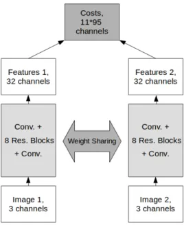
The architecture of the LDesc descriptor proposed in this work is illus-trated in figure 3.2. This architecture is partially reused from [21].

Figure 3.2: Architecture of the network.

The descriptor extracts features from 2 images using the same pa-rameters, as in Siamese networks. Thus, for each point (i, j) a feature vector f (i, j) ∈ R32 _{is obtained. The network consists of 8 residual} blocks as in figure 2.3 and 1 convolutional layer before and after the

16 CHAPTER 3. METHODS

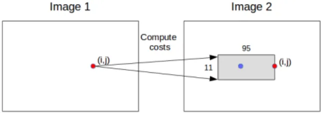
Figure 3.3: Computing matching costs.

blocks. All convolutional layers have 32 filters with kernel size 3, stride 1 and padding 1. Each convolutional layer except for the last one is fol-lowed by Batch Normalization and ReLU activation. The size of the receptive field of the network is 37× 37.

During the training, features are compared between 2 images, by computing a cost volume c:

c(i, j, k) =−∥f1(i, j)− f2(ik, jk)∥1 (3.1) where

• ∥ · ∥1is the mean absolute distance,

• k = 0, . . . window_width× window_height − 1, • ik= i +⌊k/window_width⌋ − ⌊window_height/2⌋,

• jk = j− (k mod window_width).

As illustrated in figure 3.3 each feature vector f1(i, j)from the first im-age is compared to features from the second imim-age f2(ik, jk)located in a

small widow anchored to the position (i, j). In this project window_width = 94and window_height = 11, therefore ik ∈ [i − 5, i + 5], jk∈ [j − 94, j].

For stereo images, it is known that the ground truth match for a point (i, j)is going to lie on the same axis to the left. Although this no longer holds if rotation and scaling are applied, the relative position of the window is chosen to ensure that as many ground truth matches as pos-sible are located within it. The size of the cost volume is limited by GPU memory (11GB in this project).

After computing the cost volume, sof tmax activation function to-gether with categorical cross-entropy loss is applied. This is a classi-fication task for each point, in which the location of the ground truth

CHAPTER 3. METHODS 17

match defines the correct class out of 94× 11 classes. Points, which do not have the ground truth match within the window, are filtered out and do not influence the loss function.

The training is done on 128× 256 patches, which are cropped from random positions. In addition, augmentation of the data (scaling, rota-tion and noise) is applied. Before entering the network, pixel intensities are normalized to fit the interval [−1, 1].

3.2.1 Training

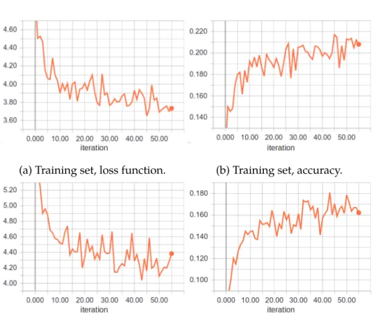
(a) Training set, loss function. (b) Training set, accuracy.

(c) Validation set, loss function. (d) Validation set, accuracy.

Figure 3.4: Training on FlyingThings.

The descriptor has been trained for approximately 50 iterations on the FlyingThings dataset, each iteration consisting of 500 training sam-ples. The model achieving the lowest validation loss (after 43 itera-tions) has been saved. Figure 3.4 shows values of the loss function and percentage of the points matched exactly (with 0 pixel error) depend-ing on iteration.

18 CHAPTER 3. METHODS

Fine-tuning on the KITTI dataset required 13 epochs.

3.3

Learning the Detector

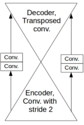
The architecture of the LDet detector proposed in this work has been partially reused from [21]. This is an encoder-decoder network, which consists of 4 convolutional and 4 transposed convolutional layers with 32 filters, kernel size 3 and stride 2. There is a residual connection between each pair of encoding and decoding layers of the same size. However, each such connection goes through 2 other convolutional layers with kernel size 3 and stride 1. This is illustrated in figure 3.5. At the end of the network there is a final convolutional layer with kernel size 3 and stride 1 that outputs only one value for each point. As a re-sult, the network consists of 4 + 2×4+1 convolutions and 4 transposed convolutions and has the receptive field of size 37× 37. All convolu-tional layers except for the last one are followed by Batch Normalization and ReLU activation, the last layer is followed by Batch Normalization and sigmoid activation and binary cross-entropy loss.

Figure 3.5: Architecture of the network.

3.3.1 Construction of the ground truth data

The key idea of this work is that the detector can be trained to predict the probability of a point being matched. This can be achieved by solv-ing a classification task with two classes, “matched” or “not matched”. The ground truth data for the detector is constructed by performing

CHAPTER 3. METHODS 19

dense point matching between images. In contrast to training the de-scriptor, all points in the first image are compared to all points in the second image (not only to points a small local window). This is done to ensure that only sufficiently unique points are matched.

A point is considered to be matched, if it’s nearest neighbor in the feature space is within one pixel distance from the ground truth (d≤ 1). Similarly, a point is considered not matched if the distance is at least 3 pixels (d ≥ 3), however all points which were matched exactly with 2 pixel error are excluded from the dataset as border-cases. The distance function is the rounded Euclidean distance as described in section 3.1.4. As comparing all-to-all is quite an expensive procedure, this is done only on centered crops of size 160× 256 for the FlyingThings dataset. However, the whole image is used for KITTI.

To force the model to better discriminate between stable and non-stable points we consider the hardest scenario and apply the maximal rotation and scaling to the second image. The scaling factor is ran-domly chosen to be either 1

1.2 or 1.2 and similarly, the rotation angle is chosen to be either−5◦or 5◦.

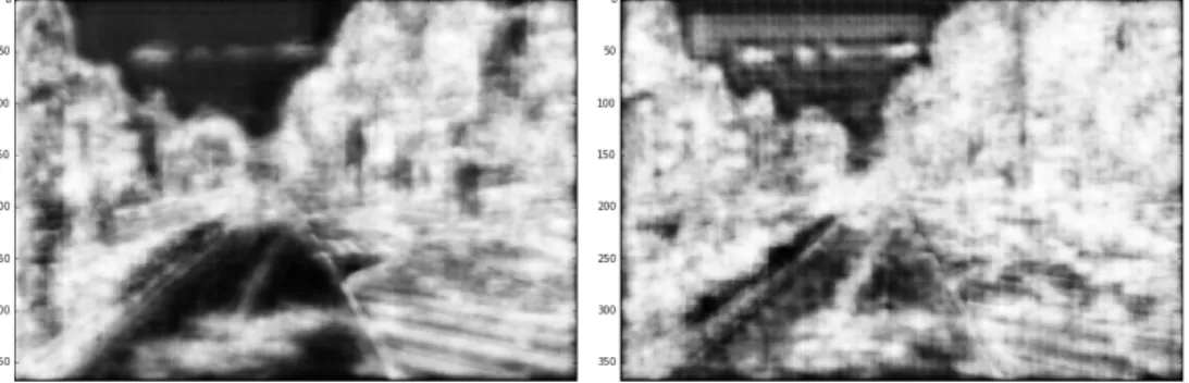
Furthermore, we have tried to add synthetic noise to the images be-fore extracting features. The figure 3.6a shows that this can produce visually more appealing results comparing to figure 3.6b as scores in the low-structured regions are smaller. However, preliminary investi-gation showed that this leads to decrease in performance on non-noisy images, therefore we chose to proceed without applying noise in train-ing the detector and leave this as a subject to further research.

While the output of the model is probability of matching, the input can be different depending on application. We tried two options. First, the detector is trained on the features extracted with the descriptor. In this case the detector inherits the invariance of the descriptor, that is important for repeatability of output scores across different frames. In the second version, the detector is trained directly from images. This allows the detection to precede the description during the inference. In this project only features from the first image in a pair contribute to the ground truth data. Figures 3.6c and 3.6d show the score maps obtained using features and the raw image as an input, respectively.

Furthermore, figures 3.6b and 3.6c reveal the difference before and after fine-tuning the model on KITTI.

20 CHAPTER 3. METHODS

(a) LDet trained on features with noise, before fine-tuning.

(b) LDet trained on features without noise, before fine-tuning.

(c) LDet trained on features, after fine-tuning.

(d) LDet trained on images, after fine-tuning.

Figure 3.6: The output of LDet – estimated probability of matching.

3.4

Point selection

Comparing all points to all is a very costly operation not feasible in practical applications. We have found that selecting local maximas from both images leads to very poor performance. Therefore, a semi-dense matching procedure is proposed: points with a score higher than a threshold are considered for matching, in addition, sparse points are selected, but only in the first image. An example of point selection is visualized in figure 3.7.

To choose sparse points the first image is split into blocks of size 2d× 2d and a point with the highest score is selected in each block. Furthermore, if two points within the distance d are selected, one of them (with a lower score) is discarded. To make fair comparison, points detected by the baseline method are also filtered, so that there are no points closer than d in the first image. However, all the points in the

CHAPTER 3. METHODS 21

(a) Sparse points selected in the first image.

(b) Dense regions selected in the sec-ond image.

Figure 3.7: Semi-dense point selection.

second image are kept. Value d = 5 is used in the experiments. Figure 3.8 provides an example.

(a) SIFT. (b) LDet.

Figure 3.8: Filtering of key-points: green – selected points, red – dis-carded points.

The score threshold 0.72 is chosen, because with this threshold the learned detector returns approximately the same amount of points in the first image as the baseline method. Also, a bit lower threshold 0.70 is applied to the second image. While from the figure 3.8 it might look like SIFT returns much more points, its important to note that only points with the existing ground truth are considered in the evaluation.

22 CHAPTER 3. METHODS

3.5

Implementation details

The described models were implemented using a deep learning frame-work Keras [5] with TensorFlow back-end [1]. All models were trained using RMSProp method [38] with default parameters (learning rate = 0.001, ρ = 0.9). However, for fine-tuning the descriptor on KITTI dataset, it was necessary to reduce learning rate to 0.0005. Relative size of the validation was 0.2 for FlyingThings and 0.1 for KITTI.

Baseline method implementations from the OpenCV library [4] were used.

Chapter 4

Results

This chapter describes evaluation experiments performed in this project and presents the results. First, the learned descriptor is evaluated sepa-rately a dense matching task. Next, the predictive power of the detector is assessed using the constructed ground truth data. Finally, both the descriptor and detector are evaluated in combination and compared against SIFT.

4.1 Descriptor

First, we compare the learned descriptor LDesc to DAISY by perform-ing dense point matchperform-ing. In this experiment each point in the first image is matched to the nearest neighbor among all the points in the second image. The percentage of correct matches is reported. Since, this is a computationally expensive experiment, it has been performed on 160× 256 image patches cropped from the image center and only 100 images from the FlyingThings test set has been used.

Table 4.1 shows the results of this experiment. Two different tol-erance levels are considered: “0p” accuracy represents the percentage of points matched exactly, while “1p” accuracy represents the percent-age of points matched within 1 pixel distance. As an exception 2 and 4 pixel accuracy is reported for KITTI Flow (please, see subsection 3.1.4). Furthermore, “+N” indicates that image samples has been augmented with random noise, “+SR” – random scaling and rotation, “+SRN” – random scaling, rotation and noise. In addition, the performance of the descriptor without fine-tuning (LDesc FT) is evaluated on KITTI.

24 CHAPTER 4. RESULTS

Table 4.1: Matching accuracy with 0 and 1 pixel tolerance. LDesc FT and LDesc KITTI represent LDesc before and after fine-tuning on KITTI respectively.

DAISY LDesc FT LDesc KITTI

Data 0p 1p 0p 1p 0p 1p FlyingThings 0.309 0.507 0.438 0.628 - -FlyingThings +N 0.149 0.368 0.176 0.392 - -FlyingThings +SR 0.088 0.317 0.221 0.524 - -FlyingThings +SRN 0.055 0.231 0.099 0.302 - -KITTI Stereo 0.204 0.558 0.360 0.754 0.382 0.782 KITTI Flow1 _{0.284 0.815 0.292 0.850 0.309 0.870} First of all, we can see from the table 4.1 that LDesc outperforms DAISY in all settings. The biggest difference in performance is in the case of FlyingThings images with additional scaling and rotation. Ac-cording to [39], DAISY handles small variations in scale and angle, but the result suggest that it is not sufficient for this experiment. In other cases, for instance, KITTI Flow and FlyingThings with noise, the results are quite similar. However, it is important to note that DAISY feature vectors consist of 200 32-bit floating point number, while LDesc – only of 32.

Secondly, the performance of the descriptor improves only slightly after fine-tuning. This could mean that either the descriptor is able to generalize from synthetic data to real images very well, or the amount of images used for fine-tuning is not sufficient to make a big difference. Figure 4.1 provides an example of dense point matching between 2 KITTI Flow images. The first image in a pair is shown together with green and red circles representing correct and incorrect matches, re-spectively. To avoid clutter we show only points, which lie on a uni-form grid with distance 7 and have the ground truth correspondences.

4.2

Detector

First of all, the detector is evaluated with respect to the ground truth data obtained as described in section 3.3.1.

The detector output for each point is a score between 0 and 1 that

CHAPTER 4. RESULTS 25

(a) DAISY (b) LDesc

Figure 4.1: Examples of dense point matching: green – correct matches, red – incorrect matches

ideally should reflect probability of match. We can assign label “matched” to all points with a score higher than a threshold t and label “not matched” otherwise. Then, we can calculate precision and recall:

precision(t) = ∑N i=1I{yi=1}× I{ ˆyi>t} ∑N i=1I{ ˆyi>t} (4.1) recall(t) = ∑N i=1I{yi=1}× I{ ˆyi>t} ∑N i=1I{yi=1} (4.2) where I{·}is an indicator function. Figure 4.2a shows a precision-recall

curve obtained by considering different values of threshold t. It shows that by increasing the threshold it is possible to filter out the points, which are going to be matched with very high precision/probability.

Furthermore, in figure 4.2b the score range is split into short contin-uous intervals and precision and recall for each interval is computed. Here, precision and recall are:

interval_precision(t) = ∑N i=1I{yi=1}× I{ ˆyi∈[t;t+δ)} ∑N i=1I{ ˆyi∈[t;t+δ)} (4.3) interval_recall(t) = ∑N i=1I{yi=1}× I{ ˆyi∈[t;t+δ)} ∑N i=1I{yi=1} (4.4) Thus, we can see that score values returned by the detector very well reflect the estimated probability of a match (precision).

26 CHAPTER 4. RESULTS

(a) Recall VS precision. (b) Interval precision and recall.

(c) Score distributions: blue - positive, red - negative, yellow - undefined.

Figure 4.2: Evaluation of the detector on FlyingThings.

Finally, figure 4.2c is a combined histogram that shows distribution of scores for positive (“matched”), negative (“not matched”) and un-defined (matched with 2 pixel error) points.

Figure 4.3 shows that similar, but less profound discrimination be-tween points is achieved on the KITTI dataset.

4.3

Combining the Descriptor and Detector

In the first experiment the accuracy of matching is evaluated for the best 100 matches, for which the ground truth data exists. If any method returns less than 100 key-points, missing key-points are counted as mis-matched. In SIFT matches are sorted according to the distance ratio between the first match and the second best match. In LDesc matches are sorted simply by the matching distance. This experiment is performed on full images, however only 500 images from the

Fly-CHAPTER 4. RESULTS 27

(a) Recall VS precision. _{(b) Interval precision and recall.}

(c) Score distributions: blue - positive, red - negative, yellow - undefined.

Figure 4.3: Evaluation of the detector on KITTI Stereo. ingThings test set are taken.

We evaluate 4 methods: • SIFT

• SIFT detector + LDesc descriptor (sparse matching) • LDesc + LDet learned from features

• LDesc + LDet learned from images The results are summarized in table 4.2.

First of all, we can see that describing points detected by SIFT with LDesc leads to better performance in all cases, except for KITTI Flow. Notably, this is the only scenario in which descriptor has not been trained. Secondly, using the learned detector improves the results even

28 CHAPTER 4. RESULTS

Table 4.2: Matching accuracy with 0 and 1 pixel tolerance for 100 points.

SIFT SIFT+LDesc LDD Feat LDD Im

Data 0p 1p 0p 1p 0p 1p 0p 1p FlyingThings 0.566 0.869 0.711 0.915 0.909 0.980 0.916 0.982 FlyingThings +SR 0.380 0.774 0.472 0.828 0.501 0.919 0.501 0.914 FlyingThings +SRN 0.200 0.567 0.251 0.599 0.290 0.636 0.218 0.494 KITTI Stereo 0.292 0.751 0.372 0.822 0.489 0.912 0.495 0.903 KITTI Stereo + SR 0.214 0.680 0.254 0.731 0.169 0.739 0.168 0.732 KITTI Stereo + SRN 0.141 0.516 0.170 0.566 0.147 0.644 0.123 0.562 KITTI Flow2 _{0.324 0.821 0.320 0.813 0.332 0.844 0.335 0.856} further. LDD Feat and LDD Im perform similarly, except for the

sce-narios with noise. This outcome has been expected, since LDD Feat uses features as input and inherits invariance to noise. On the other hand, LDD Im was trained without augmentation of the first image in a pair (which serves as input) and therefore outperforms LDD Feat in such scenarios.

Table 4.2 shows the accuracy evaluated for the best 100 matches. However, one might be interested in more or less matches depending on the application. Therefore, figure 4.4 shows average matching ac-curacy for different numbers of matches for SIFT and LDD Feat. As previously, matches are ordered by the distance ratio between the first match and the second best match for SIFT and simply by the match-ing distance for LDD Feat. We can see that LDD matches more points on average, however SIFT is better at discriminating between success-ful and unsuccesssuccess-ful matches. Therefore, in the cases with data aug-mentation SIFT shows higher accuracy when the number of considered matches is small. It is interesting that sorting by ratio is very useful for evaluating SIFT matches, but does not benefit LDD. Therefore, LDD matches were sorted simply by matching distance.

Figure 4.5 shows two examples of point matching with SIFT and LDD. The best 100 matches are shown (or less, if less key-points are detected). Green and red points represent matched and mismatched key-points, respectively. We can see that both descriptors perform well, when there is a lot of structure in the image, however, LDD is better in matching low-textured regions.

CHAPTER 4. RESULTS 29

(a) KITTI Stereo (b) KITTI Stereo +RS

(c) KITTI Stereo +RSN (d) KITTI Flow

Figure 4.4: Matching accuracy depending on the number of considered matches.

30 CHAPTER 4. RESULTS

(a) SIFT (b) LDD

(c) SIFT (d) LDD

Figure 4.5: Examples of point matching on KITTI Flow: green – correct matches, red – incorrect matches.

Chapter 5

Discussion and Conclusions

5.1 Discussion

First of all, the learned descriptor performs well in all-to-all matching task even though it has been trained by comparing features in a small local window. Moreover, it shows very good generalization capabilities from the synthetic dataset to the real data.

Secondly, the learned detector discriminates between good and bad points and can be used to discover key-points which are matched with probability higher than 90%. However, the discrimination on KITTI is not as profound as on the synthetic images. This has two potential explanations: first of all, training the detector might require more data and 200 images used for fine-tuning were not sufficient, and secondly, the detector might not generalize from the synthetic data as well as the descriptor.

Nevertheless, very promising results have been achieved by using the learned detector and descriptor in combination. Not only LDesc worked better than SIFT descriptor in our experiments, but also using LDet helped to further improve the accuracy of matching.

5.1.1 Drawbacks and future work

Apart from selecting points which are easy to match a detector must fulfill another important task – reduce the amount of points consid-ered for matching. We have found that scores predicted by LDet are to some extent repeatable across different frames, therefore the amount of points in both images can be reduced by setting a threshold.

32 CHAPTER 5. DISCUSSION AND CONCLUSIONS

ever, the scores are subjected to noise and thus selecting local maximas in both images leads to poor performance. It is possible that a differ-ent architecture for the detector in combination with a more advanced non-maximum suppression could solve this issue. Improving stabil-ity of the scores is very important, because if it was possible to select sparse repeatable points across different frames the descriptor could be applied only to those points.

Another important drawback of the method is that on a 1 core CPU LDD works approximately 100 times slower than SIFT. Of course, neu-ral networks can exploit paneu-rallelism and therefore can be executed very efficiently on GPUs, but computational complexity is still an important limitation and can prohibit execution of the method, for instance, on a mobile phone. Therefore reducing the complexity of the networks and finding a good trade-off between accuracy and time-performance is an-other subject for the future work.

Furthermore, this project focused on a limited scenario, when rota-tion and scale changed only slightly between different frames. In prac-tice it might be necessary to handle all types of variations, therefore additional improvement are necessary. For instance, including Spa-tial Transformer Layer [20] could potenSpa-tially allow to handle arbitrary changes in orientation.

Moreover, it is necessary to test the method using other datasets, for instance, datasets that contain indoor scenes, such as TUM [36] and SUN [35] RGB-D benchmarks. Furthermore, it is possible to ob-tain ground-truth correspondences between points directly from KITTI Raw video sequences [13], which would lead to much more data than is currently available in KITTI Stereo and KITTI Optical Flow bench-marks. It would be interesting to skip some frames in video sequences in order to further investigate the ability of the method to handle large viewpoint changes.

5.2

Conclusions

This work presents a novel method for key-point detection and de-scription in images. The key idea of the method is to train a descrip-tor to match points densely, then predict which points are likely to be matched and use this information for point selection. This project has shown that this approach works at least to some extent and can lead

CHAPTER 5. DISCUSSION AND CONCLUSIONS 33

to more accurate results compared to model based-methods. We hope this work will enable further research in this direction and will help to utilize the full potential of deep learning in visual odometry.

Bibliography

[1] Martı́n Abadi et al. “Tensorflow: Large-scale machine learning on heterogeneous distributed systems”. In: arXiv preprint arXiv:1603.04467 (2016).

[2] Vassileios Balntas et al. “Learning local feature descriptors with triplets and shallow convolutional neural networks.” In: BMVC. Vol. 1. 2. 2016, p. 3.

[3] Herbert Bay, Tinne Tuytelaars, and Luc Van Gool. “Surf: Speeded up robust features”. In: European conference on computer vision. Springer. 2006, pp. 404–417.

[4] G. Bradski. “The OpenCV Library”. In: Dr. Dobb’s Journal of

Soft-ware Tools (2000).

[5] François Chollet et al. Keras. https://github.com/fchollet/ keras. 2015.

[6] Christopher B Choy et al. “Universal correspondence network”. In: Advances in Neural Information Processing Systems. 2016, pp. 2414– 2422.

[7] M Bishop Christopher. PATTERN RECOGNITION AND MACHINE

LEARNING. Springer-Verlag New York, 2016.

[8] Daniel DeTone, Tomasz Malisiewicz, and Andrew Rabinovich. “SuperPoint: Self-Supervised Interest Point Detection and De-scription”. In: arXiv preprint arXiv:1712.07629 (2017).

[9] Daniel DeTone, Tomasz Malisiewicz, and Andrew Rabinovich. “Toward Geometric Deep SLAM”. In: arXiv preprint arXiv:1707.07410 (2017).

[10] Vincent Dumoulin and Francesco Visin. “A guide to convolution arithmetic for deep learning”. In: arXiv preprint arXiv:1603.07285 (2016).

BIBLIOGRAPHY 35

[11] Jakob Engel, Thomas Schöps, and Daniel Cremers. “LSD-SLAM: Large-scale direct monocular SLAM”. In: European Conference on

Computer Vision. Springer. 2014, pp. 834–849.

[12] Andreas Geiger, Philip Lenz, and Raquel Urtasun. “Are we ready for Autonomous Driving? The KITTI Vision Benchmark Suite”. In: Conference on Computer Vision and Pattern Recognition (CVPR). 2012.

[13] Andreas Geiger et al. “Vision meets Robotics: The KITTI Dataset”. In: International Journal of Robotics Research (IJRR) (2013).

[14] Xufeng Han et al. “Matchnet: Unifying feature and metric learn-ing for patch-based matchlearn-ing”. In: Computer Vision and Pattern

Recognition (CVPR), 2015 IEEE Conference on. IEEE. 2015, pp. 3279–

3286.

[15] Chris Harris and Mike Stephens. “A combined corner and edge detector.” In: Alvey vision conference. Vol. 15. 50. Manchester, UK. 1988, pp. 10–5244.

[16] Richard Hartley and Andrew Zisserman. Multiple view geometry

in computer vision. Cambridge university press, 2003.

[17] Wilfried Hartmann, Michal Havlena, and Konrad Schindler. “Pre-dicting matchability”. In: Proceedings of the IEEE Conference on

Computer Vision and Pattern Recognition. 2014, pp. 9–16.

[18] Kaiming He et al. “Deep residual learning for image recogni-tion”. In: Proceedings of the IEEE conference on computer vision and

pattern recognition. 2016, pp. 770–778.

[19] Sergey Ioffe and Christian Szegedy. “Batch normalization: Ac-celerating deep network training by reducing internal covariate shift”. In: arXiv preprint arXiv:1502.03167 (2015).

[20] Max Jaderberg, Karen Simonyan, Andrew Zisserman, et al.

“Spa-tial transformer networks”. In: Advances in neural information

pro-cessing systems. 2015, pp. 2017–2025.

[21] Alex Kendall et al. “End-to-End Learning of Geometry and Con-text for Deep Stereo Regression”. In: Computer Vision (ICCV), 2017

36 BIBLIOGRAPHY

[22] Alex Krizhevsky, Ilya Sutskever, and Geoffrey E Hinton. “Ima-genet classification with deep convolutional neural networks”. In: Advances in neural information processing systems. 2012, pp. 1097– 1105.

[23] Jonathan Long, Evan Shelhamer, and Trevor Darrell. “Fully con-volutional networks for semantic segmentation”. In: Proceedings

of the IEEE conference on computer vision and pattern recognition.

2015, pp. 3431–3440.

[24] Manolis IA Lourakis and Antonis A Argyros. “SBA: A software package for generic sparse bundle adjustment”. In: ACM

Trans-actions on Mathematical Software (TOMS) 36.1 (2009), p. 2.

[25] David G Lowe. “Distinctive image features from scale-invariant keypoints”. In: International journal of computer vision 60.2 (2004), pp. 91–110.

[26] Moritz Menze, Christian Heipke, and Andreas Geiger. “Joint 3D Estimation of Vehicles and Scene Flow”. In: ISPRS Workshop on

Image Sequence Analysis (ISA). 2015.

[27] Raul Mur-Artal, Jose Maria Martinez Montiel, and Juan D Tar-dos. “ORB-SLAM: a versatile and accurate monocular SLAM sys-tem”. In: IEEE Transactions on Robotics 31.5 (2015), pp. 1147–1163. [28] N.Mayer et al. “A Large Dataset to Train Convolutional Networks for Disparity, Optical Flow, and Scene Flow Estimation”. In: IEEE

International Conference on Computer Vision and Pattern Recognition (CVPR). arXiv:1512.02134. 2016. url: http://lmb.informatik.

uni-freiburg.de/Publications/2016/MIFDB16.

[29] Shaoqing Ren et al. “Faster r-cnn: Towards real-time object detec-tion with region proposal networks”. In: Advances in neural

infor-mation processing systems. 2015, pp. 91–99.

[30] Edward Rosten and Tom Drummond. “Fusing points and lines for high performance tracking”. In: Computer Vision, 2005. ICCV

2005. Tenth IEEE International Conference on. Vol. 2. IEEE. 2005,

pp. 1508–1515.

[31] Ethan Rublee et al. “ORB: An efficient alternative to SIFT or SURF”. In: Computer Vision (ICCV), 2011 IEEE international conference on. IEEE. 2011, pp. 2564–2571.

BIBLIOGRAPHY 37

[32] Nikolay Savinov et al. “Quad-Networks: Unsupervised Learn-ing to Rank for Interest Point Detection”. In: ProceedLearn-ings of the

IEEE Conference on Computer Vision and Pattern Recognition. 2017,

pp. 1822–1830.

[33] Johannes L Schönberger et al. “Comparative evaluation of hand-crafted and learned local features”. In: Conference on Computer

Vi-sion and Pattern Recognition (CVPR). 2017.

[34] Edgar Simo-Serra et al. “Discriminative learning of deep convo-lutional feature point descriptors”. In: Proceedings of the IEEE

In-ternational Conference on Computer Vision. 2015, pp. 118–126.

[35] Shuran Song, Samuel P Lichtenberg, and Jianxiong Xiao. “Sun rgb-d: A rgb-d scene understanding benchmark suite”. In:

Pro-ceedings of the IEEE conference on computer vision and pattern recog-nition. 2015, pp. 567–576.

[36] J. Sturm et al. “A Benchmark for the Evaluation of RGB-D SLAM Systems”. In: Proc. of the International Conference on Intelligent Robot

Systems (IROS). Oct. 2012.

[37] Jiexiong Tang, John Folkesson, and Patric Jensfelt. “Geometric Correspondence Network for Camera Motion Estimation”. In:

IEEE Robotics and Automation Letters (2018).

[38] Tijmen Tieleman and Geoffrey Hinton. “Lecture 6.5-rmsprop: Di-vide the gradient by a running average of its recent magnitude”. In: COURSERA: Neural networks for machine learning 4.2 (2012), pp. 26–31.

[39] Engin Tola, Vincent Lepetit, and Pascal Fua. “Daisy: An efficient dense descriptor applied to wide-baseline stereo”. In: IEEE

trans-actions on pattern analysis and machine intelligence 32.5 (2010), pp. 815–

830.

[40] Yannick Verdie et al. “TILDE: A Temporally Invariant Learned DEtector.” In: CVPR. Vol. 2. 4. 2015, p. 5.

[41] Kwang Moo Yi et al. “Learning to assign orientations to feature points”. In: Computer Vision and Pattern Recognition (CVPR). EPFL-CONF-217982. 2016.

[42] Kwang Moo Yi et al. “Lift: Learned invariant feature transform”. In: European Conference on Computer Vision. Springer. 2016, pp. 467– 483.

38 BIBLIOGRAPHY

[43] Sergey Zagoruyko and Nikos Komodakis. “Learning to compare image patches via convolutional neural networks”. In: Computer

Vision and Pattern Recognition (CVPR), 2015 IEEE Conference on.