The performance of GARCH option pricing models : An empirical study on Swedish OMXS30 call options

J

I

B

S

JÖNKÖPING UNIVERSITY

The performance of GARCH option pricing models

Subject: Master thesis in Finance/ Economics 2013 Author: DONALD HARDING, 1984-07-10 Tutor: Per-Olof Bjuggren, Professor

Louise Nordström, PhD candidate Jönköping May 2013

Master thesis in Finance/Economics

Title: The performance of GARCH option pricing models

Author: Donald Harding

Tutors: Per-Olof Bjuggren & Louise Nordström

Date: May 2013

Subject Terms: HestonNandi, BlackScholes, GARCH, Option pricing,

Abstract

The purpose of this thesis is to examine the properties for different specifications of the Heston and Nandis GARCH option pricing model and the pricing performance on Swe-dish OMXS30 index call options. The sample consists of a total of 2467 options (both in-sample and out-of-in-sample) for 2011 and 2012, which are priced with three specifications of the HestonNandi-GARCH model and then compared to the pricing performance of the BlackScholes model. The examination shows that the BlackScholes model performs better out-of-sample then the specifications of the HestonNandi GARCH model. All models pricing errors show significant relationship to moneyness and the term structure of the in-terest rate. We also confirm the findings of Heston and Nandi (2000) who states that their model is especially sensitive to the volatility of volatility and the skewness parameter.

Table of Contents

Abstract ... i

1

Introduction ... 1

1.1 Previous research ... 1

1.2 Purpose and problem discussion ... 3

1.3 Method... 3

1.4 Limitations ... 4

1.5 Structure ... 5

2

Theoretical framework ... 6

2.1 Risk neutral valuation ... 6

2.2 Black-Scholes option pricing model ... 6

2.3 HN-GARCH model ... 7

2.4 Heston Nandi closed-form GARCH option pricing model ... 9

2.5 Likelihood ratio test ... 9

2.6 Mispricing error measurements ... 9

2.7 Regression analysis ... 11

3

Data ... 12

4

Empirics... 14

4.1 HN-GARCH (1,1) model selection ... 14

4.2 In-sample model comparison ... 14

4.3 Out-of-sample model comparison ... 17

4.4 Regression analysis ... 21

5

Conclusion ... 23

1

Introduction

One of the most central things in financial applications and theory is the volatility, which is a vital part when considering predictions and implementation of financial models for decision-making. Since the introduction of Black and Scholes (1973) option pricing formula, researchers have tried to incorporate stochastic volatility into option pricing models. Heston (1993) introduced a closed form solution for stochastic volatility pricing of options, which Heston and Nandi (2000) later used to de-velop their Generealized Auto-Regressive Conditional Heteroscedasticity (GARCH) option-pricing model from. A common feature among all option pricing models is that they have to make basic as-sumptions about: the process of the underlying asset (the distributional properties), the volatility process and the interest rate process. The number of different combinations of the above assump-tions is continuing to increase as researchers are trying to find the “perfect model”.

The choice of model is not only about which model that predicts the price of options in the most ac-curate manner, we can also ask the question whether the implementation cost of more advanced and complex models is worth the extra gain that the potentially “perfect model” offers. This thesis will examine if the computational heavier model by Heston and Nandi (2000) is outperforming the mod-el by Black and Scholes (1973) and which pricing biases that affect the modmod-els pricing errors.

The differences between the two models lie in the previously mentioned assumptions. The first is the distributional properties, where the Black and Scholes model (BS model) assumes that the price of the underlying follows a geometric Brownian motion and that the returns are log-normally distri-buted. The Heston and Nandi model (HN model) incorporates the conditional volatility as a risk premium in order to prevent arbitrage conditions when the conditional volatility is zero, it has the ef-fect of capturing the excess kurtosis often seen in financial data by modeling the efef-fects caused by auto-regressive conditional heteroscedasticity (ARCH). The second assumption is about the variance where BS model assumes a constant variance over both time and moneyness, the HN model on the other hand models the assumed non-constant variance with a risk-neutral discrete-time GARCH-model.

1.1

Previous research

The foundation of modern option pricing and especially the Black and Scholes (1973) formula is the introduction of the Brownian motion by Louis Bachelier (1900). The Brownian motion is the first stochastic attempt to model the evolution of stock prices, which later Black and Scholes (1973) ex-plored and used as the foundation in the derivation of their well-known pricing formula.

The key assumption underlying the Black and Scholes (1973) formula is the previously mentioned geometric Brownian motion of the stock price evolution combined with a homoscedastic/finite va-riance. The Black-Scholes formula has shown to be successful in the valuation of stock option pre-miums, but Rubinstein (1985) points out some pricing biases of this model.

Rubinstein (1985) examines CBOE(Chicago Board Options Exchange) option classes and claims that the Black-Scholes formula is producing option premiums, which in a systematic pattern differs from the market prices and that these systematic pricing biases arise from the assumption of a finite variance. Rubinstein (1985) makes three conclusions about the BS pricing biases. One of his main findings is that the Black-Scholes model prices short maturity out-of-the-money options significantly higher relative to other calls.

Researchers have tried to find a model, which is not dependent on the underlying assumptions of the BS model by incorporating the heteroscedastic process of the underlying asset returns into the pric-ing formulas. The first attempts were made by Cox (1975) who introduced the constant-elasticity-of-variance model followed by the jump-diffusion model of Merton (1976) and Rubinstein’s (1983) dis-placed-diffusion model. Hull and White (1987), Scott (1987) and Wiggins (1987) all developed mod-els that are not making explicit assumptions about a finite variance. The modmod-els are instead based on the assumption that the volatility follows a stochastic process. The disadvantage of the three latest models with a stochastic volatility assumption is that they are not closed-form solutions and the im-plementation of these models requires heavy computational techniques for solving these two-dimensional differential equation systems.

Stein and Stein (1991) is similar to the BS model in the way that the stock price follows a geometric Brownian motion, but it differs significantly from the BS model by including the assumption that vo-latility is an autoregressive process in continuous time. Eisenberg and Jarrow (1994) derive a model that is similar to the model by Stein and Stein (1991) where they follow a version of the Black and Scholes (1973) model by assuming that spot prices are uncorrelated with the volatility. The models by Hull and White (1987), Scott (1987) and Wiggins (1987) are all called Stochastic Volatility (SV) models which can be divided into two subgroups, continuous time models and discrete time models. The later, a SV model in discrete time can be modeled by using the GARCH (p,q) model of Bollers-lev (1986).

The introduction of the ARCH model by Engel (1982), later generalized in a symmetric normal GARCH (p,q) model by Bollerslev (1986), opened the field for modeling/forecasting financial data with a non-constant variance and volatility clustering. Engle and Mustafa (1992) used the GARCH process of Bollerslev (1986) to conduct tests on the implied conditional volatilities of options. Apart from the previous study, the first attempt to model option prices with a GARCH (p,q) model was made by Duan (1990) who developed an option pricing model based on a GARCH (p,q) process for the underlying asset. The first risk neutral valuation of Duan (1990) was misspecified which Satchell and Timmerman (1992) and Amin and Ng (1993) pointed out.

Duan (1995) revised his findings from 1990 and specified a new model that utilized the Locally Risk-Neutral Valuation Relationship (LRNVR). He found that his GARCH option-pricing model was able to capture the changes of the conditional volatility in a parsimonious way. He also found that his GARCH model was able to capture the systematic biases of the BS model.

Heston and Nandi (2000) expand the stochastic volatility model of Heston (1993) by including a discrete time GARCH process for the underlying asset. The model by Heston and Nandi (2000) in-corporates the correlation between the spot asset returns and the historical volatility by using the dis-crete time GARCH (p,q) model. The relationship between the spot returns and the historical volatili-ty is shown to have a significant role in modeling the skewness often seen in asset returns (Heston, 1993). This differentiates the Heston and Nandi (2000) model from the BS model, since the later as-sumes continuously compounded asset returns, which are assumed to be log normally distributed with a known mean and a constant variance.

1.2

Purpose and problem discussion

As we can see from the research area of option pricing models, all option pricing models and its prices are continuous in the arguments of strike price, time to maturity, spot price, risk-free rate and volatility. But the true model is still unknown, and the problem, which all models are struggling with, is that both the volatility and the option price are unknown. This creates a forecasting problem since the true model has to make predictions about both the price and the volatility simultaneously. If the true price and the generating function would have been known we could have used the closed form model to invert the volatility.

The purpose of this thesis is to see if an implementation of an option-pricing model, that does not make specific assumptions about a constant variance and log-normally distributed returns, performs better or worse than a model that assumes that the volatility of the underlying instrument is constant. We will also try to narrow down the reasons underlying the pricing biases and what type of variables that have the largest impact on the pricing performance. The outcome of this thesis is also interest-ing since we will be able to see if the models perform in the same way on comparatively less liquid Swedish index option market as they do on the more liquid S&P500 market for which the models was created. The models are implemented during a year of highly volatile markets, which might dis-tort the results due to instability of coefficient estimates.

The result from this thesis can be used as guidance for practitioners in the process of choosing be-tween the less computational heavy Black and Scholes model and the implementation of the heavier Heston and Nandi model. The regression model will also point out variables that might improve the pricing performance of the models. These results can further be used as a suggestion for future im-provement and new research within the field of option pricing models.

1.3

Method

I have chosen to examine the pricing performance of an option pricing model that includes the time varying variance of the underlying asset, and more specifically the option pricing model of Heston and Nandi (2000). The programing language R is used for all calculations, creation of conditional subsets and graphical presentations in this thesis. I start the empirical part by filtering the data from the four criterions (see part 3). All option prices during 2011 and 2012 are filtered by moneyness, time to maturity, no-arbitrage conditions and market incompleteness.

The filtering results in a subset of 1258 options for 2011 and 1209 for 2012. Depending on the pre-vious filtering conditions a second subset is used to price the relevant options every week. I start by determining the level of asymmetry (deviation from normality) i.e. if we can see significant leverage effects in the returns of the underlying asset in order to find the most correct model for the Swedish market. The next step is then to price the models every week, two specifications of the HN-GARCH model are used in order to evaluate the performance of the model in-sample. The first model is the regular HN-GARCH (p,q) model where we estimate the coefficient over the first half of the years and keep the coefficients fixed for the whole sample period. The second model is a version of the regular HN-GARCH model, but instead of using MLE for estimating the model parameters I use a combination of a fixed multiplier and the variance of the underlying to price the subset of options. The in-sample performance of these two specifications is then compared to the in-sample perfor-mance of our benchmark model, the BS model, to determine the models ability to price options. The next step, the most interesting and also most applicable part is the performance of these HN-GARCH models out-of-sample. I use three different specifications of HN-HN-GARCH (p,q) model to test the models pricing performance out-of-sample. The first specification is the ordinary HN-GARCH (Updated) model where we use the underlying assets spot prices and fits a risk-neutral GARCH (p,q) model to the data. The second specification is the HN-GARCH (Non-updated) where we fit the same risk-neutral GARCH model to asset returns in the first half of each year and then use these coefficients for the whole out-of-sample period. The last specification of the HN-GARCH model is the HN-GARCH (Fixed) model where I fix the volatility of the volatility parameter to equal 0.1, and then use this multiplier together with the historical variance of the underlying asset to esti-mate the other parameters. I came up with this specification as an alternative to the ordinary model in turbulent markets. The idea origins from the findings by Heston and Nandi (2000) who claims that their model is quite sensitive to changes in the volatility of volatility and the skewness parameter. In order to exclude this sensitivity biases I fix the volatility of volatility to 0.1 to see how the pricing performance changes if we would have had a more stable parameter. The models, both the GARCH specifications and the BS model, are evaluated out-of sample, where the previous observations in that year are used as a sample to estimate the conditional variance for the GARCH coefficients and the historical variance for the BS model every week in the second half of each year.

The models are then compared from their ability to value option towards the midprice of the bid/ask-spread. These errors are then used as the dependent variable in the regression model speci-fied by Bakshi, Cao and Chen (1997) to see if we can draw any conclusion about the pricing biases and whether these are due to contract specific variables or to dynamically changing market condi-tions.

1.4

Limitations

The limitations of this study are that Heston and Nandi (2000) uses both maximum likelihood esti-mation (MLE) and Non-linear least squares (NLLS) to estimate the GARCH coefficients, while this study only uses MLE. Another limitation is that this study excludes data for the dividend paying months of the index in order to model the underlying correctly. This means that since dividends are mostly paid-out in April and May, these months are excluded.

1.5

Structure

The second part of this thesis consists of a theoretical framework, which explains the underlying models and their implicit assumptions, and it aims at giving the readers a thorough understanding of the differences between the models and its respective components. The third part contains a descrip-tion of the data used in this thesis and the selective restricdescrip-tions imposed on it. The fourth part begins with unit root testing of the different data sets in order to ensure stationarity. It also contains both the in sample and out of sample estimation combined with the respective mispricing errors. And the last part, part 5 summarizes the findings of part 4 in a conclusion.

2

Theoretical framework

This section presents the models used and the final equations on which the models are built upon. It will also give an explanation of the pricing performance measurements used to evaluate the different models.

2.1

Risk neutral valuation

The foundation of risk neutral valuation, as used in option pricing, lies in the martingale measure-ment by Levy (1934). A martingale in probability theory is a model that can be used to model a fair game where no winning strategies can be used since the probability of an event is based on a stochas-tic process where the expected next value is equal to the probability of the present value.

The risk-neutral measurement is apart from the martingale process, based on the fundamental theo-rem of arbitrage where we assume that there are no arbitrage opportunities if the risk neutral distri-butional properties are equal to the distridistri-butional properties of the underlying asset. The fundamental theorem of arbitrage also implies that if there is only one risk free measure there will exist one unique price for every asset in complete markets.

Hull (1987) shows that the option price from the BS model holds if the stock price and the volatility are uncorrelated in a risk-neutral world. He also shows that the option price is true in a risky world as well if the previously mentioned uncorrelated variables are uncorrelated with aggregate consumption. Cox and Ross (1976) further argue that if the above is true, the variables in the BS model are inde-pendent of the individual risk preferences in the market, which also indicates that all investors are risk-neutral. According to Rubinstein (1985) this assumption simplifies the pricing of options, and especially the movement between spaces with different risk preferences. Hull (2006) presents that the movement between different risk spaces is not affecting the option price since the move from, for example a risk neutral world to a risky world, only changes two variables which offset each other. The offsetting change happens between the expected growth rate of the underlying and the discount rate, which is shown by Cox and Ross (1976) who says that the expected rate of return is equal to the risk free rate in a risk neutral world i.e. the price of the asset is equal to the expected payoff dis-counted at the risk-free rate.

2.2

Black-Scholes option pricing model

The option-pricing model for non-dividend paying stocks, introduced by Black and Scholes in 1973, has turned out to be the most widely used model for option pricing. It has been shown that the model suffers from strong underlying assumptions. The two major assumptions are that the model assumes the volatility of the underlying instrument to be constant and that the returns of the same are log-normally distributed. These two assumptions are quite severe and Black (1976) even con-demns the model as wrong if the volatility of the underlying changes over time. The assumption that returns are log-normally distributed is also a strong assumption to make since it has been shown in many papers that financial data suffers from excess Kurtosis (Fama, 1965 and Mandelbrot, 1963) i.e. “fat tails” which often can be related to ARCH effects. The derivation of the option pricing formula

can be found in almost all economics/finance literature and will therefore not be presented here. Black and Scholes final model for an option on a non-dividend paying stock is as follows:

Where

Where C is the premium of an European call option, is the spot price of the underlying at time t, is a standard normal random variable with the value d1, K is the strike price, r is the risk-free rate, (T-t) is the time to maturity and is the annualized volatility.

The volatility for the BS model is estimated following both Iacus (2011) and Wuertz (2012), where the volatility used to price the options is equal to annualized volatility of the underlying asset.

Where is the standard deviation of the return series and 252 is the average number of trad-ing days in a year.

2.3

HN-GARCH model

The HN-GARCH (p,q) model is based on two assumptions where the first is that the underlying spot price ( ) follows a GARCH process with as the size of time steps. The mean model (5) and the stochastic volatility model (6) are defined as below:

Where r is the continuously compounded interest rate for the time interval of size , is the condi-tional variance, is a constant parameter representing the risk neutral valuation relationship and is a standard normal disturbance term. Even though equation 6 is quite similar to Bollerslevs (1986) GARCH (p,q) model it has some distinct differences and is more similar with the NGARCH and VGARCH introduced by Engle and NG(1983). The model also incorporates the non-arbitrage con-dition of option pricing by including the concon-ditional variance in the mean equation as a risk-premium.

Moreover the GARCH process is considered stationary if the following condition is fulfilled:

Heston and Nandi (2000) arrives at the following final risk-neutral GARCH (p,q) model where is equal to -0.5: Where:

The difference between equations 5,6 and 7,8 is that 5 and 6 are risk-neutral versions of 7 and 8. The second assumption is that the value of a European call option with only one period to maturity “obeys the Black-Scholes-Rubinstein formula” (Heston and Nandi, 2000). This is shown in their pa-per and used to derive the final model for pricing of European call options. The option pricing mod- el of Heston and Nandi is presented in the next section.

2.4

Heston Nandi closed-form GARCH option pricing model

Heston and Nandi (2000) derives a closed-form option pricing model that presents option values as functions of today’s underlying spot prices and the history of the underlying’s historical prices. The difference between their model and the model presented by Heston (1993) gets very small as ap-proaches one day.

This thesis will only present the outcome (the final models) and not the whole derivation of the ge-nerating functions or the convergence to a continuous time function. For complete derivations see Heston and Nandi (2000). Heston and Nandi (2000) present the following model for pricing of Eu-ropean call options at time t with strike price (K) and time to maturity T-t.

Where C is the option premium, r is the risk-free rate and is the expectations under a

risk-neutral valuation.

2.5

Likelihood ratio test

I use the Likelihood-Ratio test in order to statistically see if the parameter that controls the skewness ( ), is significant or not. The Likelihood-Ratio test (LR test) is calculated as:

Where is the Log-likelihood of the un-restricted model (Asymmetric GARCH ( ))

and is the Log-likelihood of the restricted model (Symmetric GARCH ( )). The test statistic (LR) is Chi-squared distributed with number of restrictions as degrees of freedom under the null hypothesis. If we find that is significantly different from zero it would imply that the data is not symmetrically distributed around the mean. This would imply that the data is not normally distri-buted.

2.6

Mispricing error measurements

I use the Root Mean Squared Error (RMSE) as a comparison number for the models ability to price options. The RMSE is used since it measures the squared errors between the model price (HN or BS) and the market price, which is the mid-price of the bid/ask spread.

Where N is the number of observations in our sample, is the calculated price from the model and is the mid-price of the bid ask spread. The RMSE has the characteristic of being more pu-nitive to larger mispricing errors since the pricing error is squared before it is averaged, which means that it assigns higher weights to larger errors.

In order to capture the average mispricing that occurs outside the bid/ask spread I use the Mean Outside Pricing Error (MOE). The MOE is equal to the difference between the model price ( and the ask price ( if the models value exceeds the ask price. If the models value is smaller than the bid price ( , the MOE is equal to the difference between the model value and the bid price. The third and final condition is that if the model value falls inside the bid/ask spread the MOE is equal to zero. The MOE is used to see if the models systematically misprice the options and whether we can see any patterns of the direction of the mispricing.

The third and last pricing measurement is the Mean Absolute Error, which measures the average of the absolute mispricing error. The measurement is very similar to the MOE but instead of analyzing the direction of the error the MAE measures the absolute value of the mispricing.

2.7

Regression analysis

In order to see if the models mispricing is due to contract specific variables or to the dynamically changing market conditions we estimate a regression with percentage error ( as the depen-dent variable for each year and model. I follow the model specified by Bakshi, Cao and Chen (1997):

(16) Where is the ratio of the spot price, of the underlying, and the strike price for op-tion n at time t, is the time to maturity of option n in years, (t) is the percentage spread between the bid and the ask price of option n at time t, represents the spread between the 3-month Swedish treasury bill and the 6 3-month treasury bill and is previous observation of the volatility (annualized) to that estimation point.

The variables , and are contract specific variables, which measures the option pricings models sensitivity to these parameters. and on the other hand measures the models sensitivity to changes in market conditions.

3

Data

This study uses daily data from European call options on the OMXS30 index between 2011 and 2012. The daily closing prices for the index, the bid/ask prices for the options and the 90-day Trea-sury Bill used as the risk free rate are all collected from ThomsonReuters Datastream.

I follow Dumas, Fleming and Whaley (1998) who suggests a way to create weekly data by filtering the daily observations. The daily observations of the options are sampled once a week to create weekly observations. Tuesdays are chosen for 2011 and Thursdays for 2012 as the days when the op-tions are sampled and priced since these are the days with the fewest amount of holidays in the re-spective year. If the market is closed on these days, the next trading day will be chosen. This only oc-curs one time during both years (NasdaqOMX, 2011, 2012).

I follow Dumas, Fleming and Whaley (1998) and use these three criterions, initially, to create a sam-ple of options to price each week:

1. Only options with an absolute moneyness less than or equal to ten percent is used.

2. The second is that only options with maturity between 6 and 100 days are used in the sample.

3. The third restriction is that option prices have to obey the non-arbitrary condition by Merton (1973).If the non-arbitrary condition is exceeded it would mean that investors could build an arbitrage portfolio with a short position in the underlying, a long position in a European call option on the same underlying and invest the present value of the exercise price (K) in the risk-free rate. To avoid this, the following condition has to hold:

Where S is the spot price of the underlying, K is the strike price, r is the risk-free rate and T-t is the time to maturity measured in years.

The midprice between the bid/ask prices is used as market price to evaluate the pricing performance of the respective model. Due to the incompleteness of a bid/ask spread, which is due to low market liquidity in options with long time to maturity, the following restrictions are imposed on the mid-price:

In order to avoid inference with the non-arbitrary condition, all midprices that are equal to zero are excluded from the dataset.

4

Empirics

4.1

HN-GARCH (1,1) model selection

Similarly to Heston and Nandi (2000) I start with two different HN-GARCH (1,1) models, the sym-metric and the asymsym-metric but unlike HN I use only the Maximum likelihood estimation (MLE) to estimate both the symmetric ( ) and the asymmetric ( ) GARCH (1,1) models.

The data used to estimate the in-sample coefficients for both models are the stationary daily log-returns of the index for 2011 and 2012. The return series for both years are tested to ensure statio-narity following the Elder and Kennedy (2001) approach. The two models are then evaluated in or-der to test the significance of the skewness parameter ( ), which is included in order to capture le-verage effects in the data.

Table 2: Maximum likelihood estimations of HN-GARCH (1,1) model

GARCH-model Log-Likelihood Persistence

2011 Symmetric 0.00002134 0.9194 0 5.057E-16 -0.554 25.83% 1319.86 0.919432 Asymmetric 0.00001158 0.8205 105.3 1.56E-251 -0.897 23.89% 1324.98 0.948968 2012 Symmetric 0.00000446 0.9658 0 3.92E-13 4.41 18.14% 1381.70 0.965783 Asymmetric 0.00000601 0.7332 193.4 9.27E-130 2.27 18.94% 1389.21 0.957714

Note: Teta (Long-run volatility) is calculated as . The conditional variance is said

to be integrated (non-stationary) if the persistence, measured by . The half life period (HLP) is the

num-ber of time periods it takes for a shock to be reduced by 50% and is calculated as, .

The critical value for the Chi-square distribution with one degree of freedom at the five percent sig-nificance level is 3.84, which makes us reject the null hypothesis of a symmetric GARCH model since the LR-test statistic for 2011 is 10.24 and 15.02 for 2012. This implies that the skewness para-meter ( ) is significant for both years and that we have a negative correlation between the returns and the variance, i.e. presence of leverage effects in the data. Both the restricted (Symmetric GARCH) and the unrestricted (Asymmetric GARCH) model show a mean reverting process for both 2011 and 2012 since the persistence is smaller than one. The Half-life period (HLP) measures the memory of the mean reverting process after a shock, and it takes 13.23 days and 16.04 days for 50% of a shock to die out in 2011 and 2012. The volatility of volatility measured by is 1.158e-05 and 6.01e-06 for 2011 and 2012 respectively, and the long run mean of annualized volatility meas-ured by is 23.89% and 18.94% respectively.

4.2

In-sample model comparison

The in-sample model comparison of the BS and the asymmetric HN-GARCH (1,1) is based on data for the first half of each year, 2011 and 2012. The HN-GARCH (1,1) model is estimated using MLE on daily index returns during the same time period.

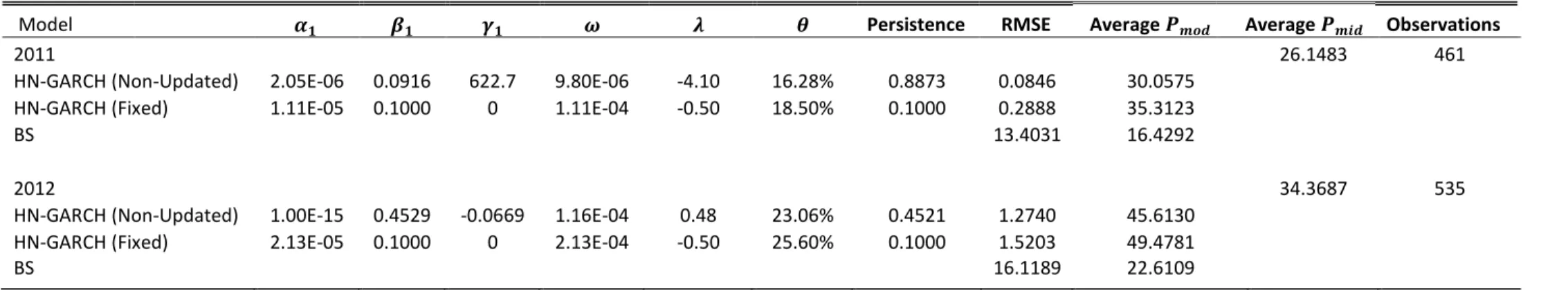
The volatility of the BS model and the HN-GARCH coefficients are held constant for the whole pe-riod (first six months of each year). Table 3 shows the coefficients from the asymmetric HN-GARCH and the fixed coefficient HN-HN-GARCH estimations, the RMSE for each model and the av-erage of the respective models prices and number of observations.

Figure 1a: Conditional Variance 2011 Figure 1b: Conditional Variance 2012

We can see from the in-sample estimations in Table 3 that the long run annualized volatility is quite similar between the models in the respective years. The asymmetric HN-GARCH model seems to be able to price the options in the most correct manner in both years since the RMSE measurements is minimized when this model is selected, this is also confirmed since the average price of this model is closest to the average mid-price. Both HN-GARCH models are outperforming the BS model signifi-cantly for the in-sample estimations and we can see that the asymmetric model has a lower , which measures the volatility of volatility than the fixed coefficient model. The stability of and is im-portant for the respective HN-GARCH model to fit the time-series of returns well (Heston and Nandi, 2000). Figure 1a and 1b shows the conditional standard deviations for each respective year, and we can see that the coefficient is relatively stable during the sample for both 2011 and 2012, which improves the pricing performance of the HN-GARCH model. Table 3 also shows that the skewness parameter is highly significant for 2011 while we might suspect that the same parameter for 2012 is not, due to the low value (-0.0669).

Trading day C o n d it io n a l V a ri a n c e 0 50 100 150 200 250 1 e -0 4 3 e -0 4 5 e -0 4 7 e -0 4 Trading day C o n d it io n a l V a ri a n c e 0 50 100 150 200 250 1 e -0 4 2 e -0 4 3 e -0 4 4 e -0 4

Table 3: Maximum likelihood in-sample estimations

Model Persistence RMSE Average Average Observations

2011 26.1483 461

HN-GARCH (Non-Updated) 2.05E-06 0.0916 622.7 9.80E-06 -4.10 16.28% 0.8873 0.0846 30.0575

HN-GARCH (Fixed) 1.11E-05 0.1000 0 1.11E-04 -0.50 18.50% 0.1000 0.2888 35.3123

BS 13.4031 16.4292

2012 34.3687 535

HN-GARCH (Non-Updated) 1.00E-15 0.4529 -0.0669 1.16E-04 0.48 23.06% 0.4521 1.2740 45.6130

HN-GARCH (Fixed) 2.13E-05 0.1000 0 2.13E-04 -0.50 25.60% 0.1000 1.5203 49.4781

BS 16.1189 22.6109

Note: The table shows the coefficients for the HN-GARCH fitting of the data in the first half of each year. The HN-GARCH (Fixed) model is a symmetric model

spe-cification of the HN-GARCH model with fixed coefficient for , and parameter that is the result of the variance of the underlying returns and .The BS model is

4.3

Out-of-sample model comparison

The out-of-sample calculations of the option price is done by a re-estimation of the HN-GARCH(1,1) model every week where the previous observations to that day of each year are used as sample size for the estimations of coefficients. The volatility used to calculate the BS-option price is calculated using the same sample of returns from the start of each year to that day.

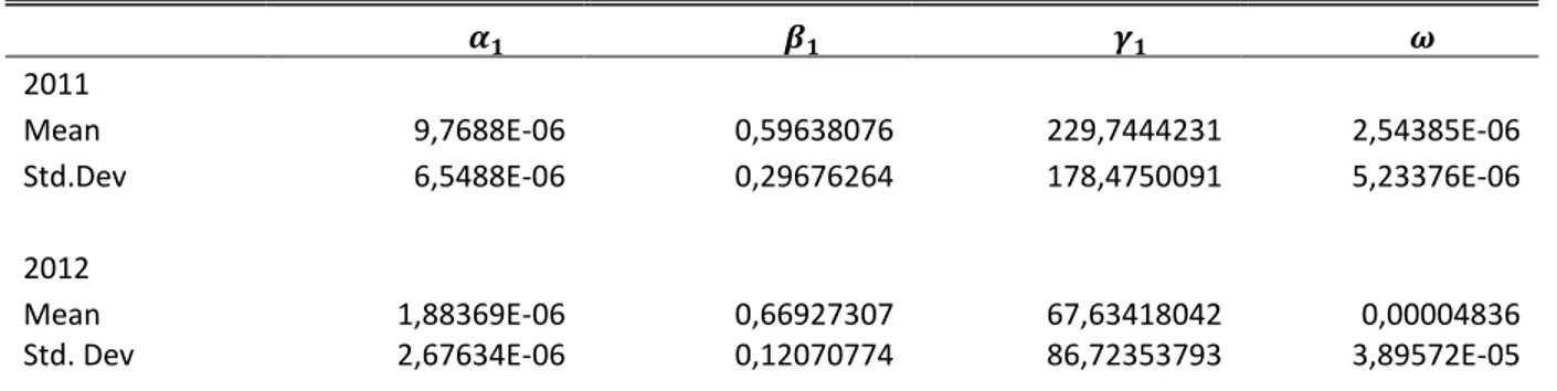
We can see from Table 4 below, which shows the coefficient estimates for the HN-GARCH(1,1) model estimated every week in the second half of each year, that the most stable parameter is . The least stable parameters are and. , which also is the HN-GARCH models most sensitive pa-rameters. The stability of the and are very important in order for the GARCH model to fit the

data in a good way.

Table 4: Mean estimates from the updated HN-GARCH(1,1) model

2011

Mean 9,7688E-06 0,59638076 229,7444231 2,54385E-06

Std.Dev 6,5488E-06 0,29676264 178,4750091 5,23376E-06

2012

Mean 1,88369E-06 0,66927307 67,63418042 0,00004836

Std. Dev 2,67634E-06 0,12070774 86,72353793 3,89572E-05

Note: This table reports the mean and standard deviation of the Out-of-sample HN-GARCH (1.1) coefficients for the updated model where the coefficients are estimated every week. The coefficients are obtained by using Maximum Likelihood estimation (MLE).

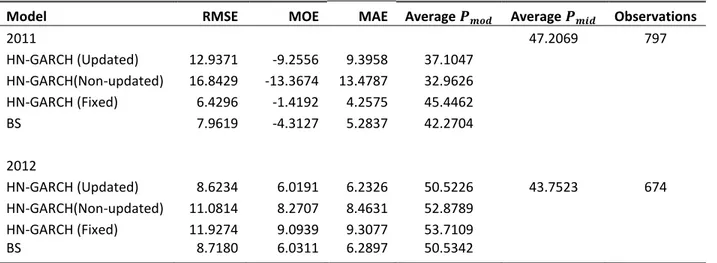
Table 5 shows the out-of-sample mispricing error measurements divided by year, and we can see that only the HN-GARCH (Fixed) model outperforms the BS model significantly during 2011. The aver-age model price for the HN-GARCH (Fixed) model is relatively close to the averaver-age midprice during this year, which is an indication of the models ability to fit the data. All models are underpricing more than they are overpricing in 2011, which is an indication of the markets expectations of an in-crease in volatility in the second part of the year. The underpricing arises from the fact that the va-riance is estimated over historical spot prices while the volatility in the market is increasing. The re-versed relationship can also be seen in the output for 2012 where all models overprice more than they are underpricing which can be related to the increase in volatility in the second part of 2011. The models use the historical volatility to model the option prices, but they are then overestimating the volatility due to higher levels in previous spot prices. These mispricing errors can also be ex-plained by the instability of the parameter during the end of 2011 and beginning of 2012. The un-derestimation in 2011 and the overestimation of the volatility in 2012 can be seen in Table 3, where the measurement of the long-run annualized volatility is significantly higher in 2011 than in 2012. We can also spot the instability of the parameter in Figure 1a and 1b where the increase in volatility of the conditional variance can be seen in the second part of 2011 and the relatively high volatility in the first part of 2012 compared to the second part.

Table 5: Out-of-sample estimates

Model RMSE MOE MAE Average Average Observations

2011 47.2069 797 HN-GARCH (Updated) 12.9371 -9.2556 9.3958 37.1047 HN-GARCH(Non-updated) 16.8429 -13.3674 13.4787 32.9626 HN-GARCH (Fixed) 6.4296 -1.4192 4.2575 45.4462 BS 7.9619 -4.3127 5.2837 42.2704 2012 HN-GARCH (Updated) 8.6234 6.0191 6.2326 50.5226 43.7523 674 HN-GARCH(Non-updated) 11.0814 8.2707 8.4631 52.8789 HN-GARCH (Fixed) 11.9274 9.0939 9.3077 53.7109 BS 8.7180 6.0311 6.2897 50.5342

Note: All mispricing measurements and option prices are measured in SEK. The option prices of the different models underlying the valuation errors are calculated by estimation of the volatility each week.

The pricing performance of the HN-GARCH specifications and the increase in pricing errors, espe-cially the RMSE measurement, from the in-sample estimations of Table 3 can apart from the natural estimation differences of the in-sample and out-of-sample predictions, be explained by the structure of the conditional variance in Figure 1a and 1b.

Table 6 shows the out-of-sample pricing errors for the different models divided by moneyness inter-vals and maturity for both 2011 and 2012. The models are performing significantly better when it comes to Out-of-the-money call options and the pricing errors increase as the options goes deeper and deeper in the money. The HN-GARCH (Fixed) model is the best performing model when it comes to deep-out-of-the-money options for both short and medium term. And since the HN-GARCH (Updated) model is underpricing over all maturities, it confirm the previous believes stated about the HN-GARCH (Updated) models sensitivity to the instability of the parameter since when we fix the coefficient in the HN-GARCH (Fixed) model we reduce the negative pricing errors. All models are showing an increase in the valuation errors as we increase the time to maturity from short-term options (6<T<40) to long-term options (70<T<100). In line with the findings of Rubins-tein (1985), the BS model is underpricing deep-out-of-the money options.

Figure 2a-c are graphical demonstrations of the models percentage errors over moneyness. The fig-ures clearly show that the BS model produces the lowest pricing errors over all maturities followed by the HN-GARCH (Fixed) model and the HN-GARCH (Updated) model.

Table 6: Out-of-sample valuation errors

Note: The percentage errors are calculated as:

where is the average midprice for the options with this maturity. Moneyness is calculated as (K/S) where K is the strike price and S is the spot price of the

6-40 40-70 70-100

Model Moneyness RMSE %Error MOE RMSE %Error MOE RMSE %Error MOE

HN-GARCH 0.90-0.95 6.4826 7.7974 -2.3844 9.0114 9.6623 -3.2936 10.0087 9.9878 -3.6870 0.95-0.99 8.9103 19.2309 -2.8474 13.3188 22.0126 -4.7627 15.0391 21.8705 -4.5492 0.99-1.01 10.0158 37.6356 -1.9651 15.2359 35.5615 -4.6616 16.7967 32.5145 -3.8221 1.01-1.05 9.6986 69.3245 -1.9074 14.9919 55.1522 -3.1326 17.1298 47.9407 -2.3053 1.05-1.10 5.5429 136.3144 -0.5560 11.3087 107.8929 0.6962 14.1302 84.0344 2.5108 HN-GARCH(Non-Updated) 0.90-0.95 8.2613 9.9369 -3.3516 12.0973 12.9711 -3.9611 14.0572 14.0279 -4.1079 0.95-0.99 11.8310 25.5346 -4.6504 17.8467 29.4958 -6.7632 19.5806 28.4749 -5.9504 0.99-1.01 13.6952 51.4613 -4.3502 20.0332 46.7588 -7.0774 21.9633 42.5159 -6.0612 1.01-1.05 12.5361 89.6069 -3.4354 18.8958 69.5139 -4.8283 21.5426 60.2907 -4.2092 1.05-1.10 7.0279 172.8338 -0.7136 13.9937 133.5094 0.7266 17.7283 105.4332 1.8627 HN-GARCH F 0.90-0.95 5.6551 6.8022 -0.8322 7.0103 7.5166 0.2898 8.4466 8.4289 1.2256 0.95-0.99 7.1856 15.5085 0.9208 9.5802 15.8335 2.3907 11.7276 17.0547 2.9749 0.99-1.01 8.2576 31.0289 3.4495 11.0995 25.9070 4.3778 13.0833 25.3262 5.1104 1.01-1.05 8.1398 58.1824 3.9639 11.8097 43.4458 6.6825 14.2003 39.7419 7.4089 1.05-1.10 5.4682 134.4764 3.2110 11.0389 105.3182 8.4490 14.6959 87.3993 10.6563 BS 0.90-0.95 6.0695 7.3006 -2.1279 7.2879 7.8144 -2.5312 8.2416 8.2244 -2.6592 0.95-0.99 7.1572 15.4472 -1.2134 9.2949 15.3619 -1.3357 11.1769 16.2539 -1.7305 0.99-1.01 7.4193 27.8787 0.8872 10.0480 23.4527 0.4715 11.7472 22.7398 0.2869 1.01-1.05 7.0491 50.3862 1.5209 9.8459 36.2209 2.6844 12.0058 33.6004 2.5764 1.05-1.10 4.2761 105.1594 1.5785 8.4278 80.4067 5.0895 11.4276 67.9616 6.2692

Figure 2a

This figure presents the out-of-sample percentage valuation errors for options with maturity between 6 and 40 days in the second half of each year. HN-GARCH (Non-updated) is the model with coefficients estimated in the first half of each year. HN-GARCH (updated) is the model where the coefficients are estimated every week, HN-GARCH (Fixed) is the model where we re-estimate the coefficients every week but use a multip-lier and the historical volatility to estimate the coefficients. BS is the Black-Scholes model, which uses the his-torical volatility, updated every week.

Figure 2b

This figure presents the out-of-sample percentage valuation errors for options with maturity between 40 and 70 days in the second half of each year. HN-GARCH (Non-updated) is the model with coefficients estimated in the first half of each year. HN-GARCH (updated) is the model where the coefficients are estimated every week, HN-GARCH (Fixed) is the model where we re-estimate the coefficients every week but use a multip-lier and the historical volatility to estimate the coefficients. BS is the Black-Scholes model, which uses the his-torical volatility, updated every week.

Moneyness O u t-o f-s a m p le % E rr o r 0.9-0.95 0.95-0.99 0.99-1.01 1.01-1.05 1.05-1.10 0 20 40 60 80 100 120 140

160 HN-GARCH (Non-updated)HN-GARCH (Updated) HN-GARCH (Fixed) BS Moneyness O u t-o f-s a m p le % E rr o r 0.9-0.95 0.95-0.99 0.99-1.01 1.01-1.05 1.05-1.10 0 20 40 60 80 100 120 HN-GARCH (Non-updated) HN-GARCH (Updated) HN-GARCH (Fixed) BS

Figure 2c

This figure presents the out-of-sample percentage valuation errors for options with maturity between 70 and 100 days in the second half of each year. HN-GARCH (Non-updated) is the model with coefficients esti-mated in the first half of each year. HN-GARCH (updated) is the model where the coefficients are estiesti-mated every week, HN-GARCH (Fixed) is the model where we re-estimate the coefficients every week but use a multiplier and the historical volatility to estimate the coefficients. BS is the Black-Scholes model, which uses the historical volatility, updated every week.

4.4

Regression analysis

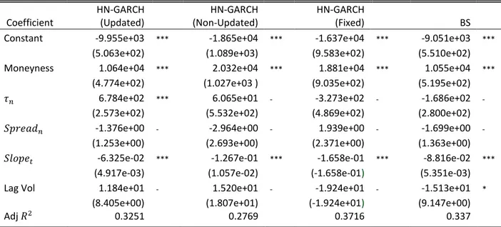
Following the methodology of Bakshi, Cao and Chen (1997), I estimate a regression model with the percentage errors of each option pricing model as the dependent variable and dif-ferent contract specific and market conditions dependent variables as the independent va-riables. The output from the pricing error regression is shown in Table 7 with the coeffi-cient estimates, its respective significance level and standard error.

We can see that all models suffer from pricing biases that arise from two main variables, moneyness and the spread of Swedish 3-month and 6-month treasury bills. The pricing er-rors from the HN-HARCH (Updated) model have apart from the other models also a sig-nificant relationship with the time to maturity of the options. The coefficient for the signif-icant time to maturity coefficient of the HN-GARCH (Updated) model indicates that an increase of one week on the time to maturity would also increase the pricing error of the HN-GARCH (Updated) model by 13 percent. Both the Moneyness and Time-to-maturity variable are contract specific errors, which are related to cross-sectional pricing biases (Bak-shi, Cao and Chen, 1997). All models have positive signs for the Moneyness coefficient, which is what we would expect since an increase of the Moneyness parameter, as we can see in Figure 2a-c, increases the pricing error significantly especially as the options becomes deeper in-the-money. Moneyness O u t-o f-s a m p le % E rr o r 0.9-0.95 0.95-0.99 0.99-1.01 1.01-1.05 1.05-1.10 0 20 40 60 80 100 HN-GARCH (Non-updated) HN-GARCH (Updated) HN-GARCH (Fixed) BS

Table 7: Coefficient estimates from the pricing error regression

Note: Coefficients are based on the combined out-of-sample for 2011 and 2012. The numbers within paren-thesis are the standard errors for each respective coefficient. ***, ** and * represent the following significance levels 0.01, 0.05 and 0.1.

The variable on the other hand is related to changes in market conditions and re-flects the different models ability to capture changes in the risk-free yield between 3-months and 6-3-months Swedish treasury bills and how this affects the pricing performance. The coefficient is significant for all models which is what we might expect since no model is incorporating the term-structure of the interest rate. The negative relationship be-tween the interest rate yield and the pricing errors indicates that increases in the spread would help improve the pricing performance of all models.

All models have quite high R-square compared to the result of Bakshi, Cao and Chen, 1997 who performed regression analysis on the pricing errors of stochastic volatility models. HN-GARCH (Fixed) has the highest R-square, 0.3716, while the non-updated version has lowest at 0.2769. Coefficient HN-GARCH (Updated) HN-GARCH (Non-Updated) HN-GARCH (Fixed) BS

Constant -9.955e+03 *** -1.865e+04 *** -1.637e+04 *** -9.051e+03 ***

(5.063e+02) (1.089e+03) (9.583e+02) (5.510e+02)

Moneyness 1.064e+04 *** 2.032e+04 *** 1.881e+04 *** 1.055e+04 ***

(4.774e+02) (1.027e+03 ) (9.035e+02) (5.195e+02)

6.784e+02 *** 6.065e+01 - -3.273e+02 - -1.686e+02 -

(2.573e+02) (5.532e+02) (4.869e+02) (2.800e+02)

-1.376e+00 - -2.964e+00 - 1.939e+00 - -1.699e+00 -

(1.253e+00) (2.693e+00) (2.371e+00) (1.363e+00)

-6.325e-02 *** -1.267e-01 *** -1.658e-01 *** -8.816e-02 ***

(4.917e-03) (1.057e-02) (-1.658e-01) (5.351e-03)

Lag Vol 1.184e+01 - 1.520e+01 - -1.924e+01 - -1.513e+01 *

(8.405e+00) (1.807e+01) (-1.924e+01) (9.147e+00)

5

Conclusion

The purpose of this thesis is to examine the properties and pricing performance of two dif-ferent methods/models used to price options. The literature on option pricing models is increasing as researcher and practitioners are continuing the search for a perfect model. We examine two models with different underlying assumptions, the BlackScholes model and the HestonNandi GARCH option-pricing model. The two models differ in many ways but the main difference lies in the estimation of the volatility used in pricing models. Pricing of options in illiquid markets and non-traded options complicates the estimation of the im-plied volatility since it cannot be estimated from the BlackScholes model due to the lack of option prices. This is often the case for long-term OMXS30 options (70<T), and this thesis therefore uses the historical volatility of the underlying asset instead of the implied volatili-ty. The process of the variance for the underlying asset, the Swedish stock index, is also used to model the HestonNandi discrete time GARCH model (HN-GARCH) for Euro-pean call options. Apart from the original specification made by Heston and Nadi (2000), who uses both Non-Linear Least Squares and Maximum likelihood estimation (MLE), this thesis only considers parameter fitting by MLE.

The empirical results are based on the single lag HN-GARCH (1,1) and the BS model dur-ing 2011 and 2012. The results show that the BS model outperforms the HN-GARCH specifications over all maturities and moneyness except for the deep-out-of-the-money short and medium term options. The specification of the HN-GARCH model that per-forms best is my own specification, the HN-GARCH (Fixed) model, which can be ex-plained by a relatively unstable volatility of volatility coefficient. We can conclude that the BS model performs better than the HN-GARCH model in markets with unstable condi-tions using MLE to fit the coefficients. This is in line with the findings of Heston and Nandi (2000) who finds that in order for the GARCH model to fit the data in a good way, it is crucial to have stable skewness and volatility of volatility coefficients. This further in-dicates that the more computational heavy model, the HN-GARCH model, is not a good choice since the Black and Scholes model outperform all stochastic volatility specifications. Due to the costs associated with more complex models there is no reason for implementa-tion of such a model on the Swedish market using MLE to fit the GARCH models during highly volatile market conditions.

The regression output show that all pricing errors are significantly affected by the contract specific variable moneyness, and the term-structure of the interest rate, which is a measure of the models sensitivity to dynamically changing conditions in the market. The pricing er-rors of the HN-GARCH (Updated) model also showed significant relationship with the contracts time to maturity and the BS model showed a small significance with the lagged volatility.

An improvement and interesting result would be the inclusion of a NLLS GARCH model, which most likely would improve the performance of the HN-GARCH (Updated) model significantly since the use of a non-linear model would incorporate the non-linear expecta-tions that can be seen in the markets. It would also be interesting to incorporate the model-ing of the interest rates term-structure, which showed to be highly significant for all mi-spricing errors.

References

Amin K, Ng V, 1993, ARCH process and option valuation, Working paper, University of Mich-igan,

Bachelier L, 1900, Théorie de la speculation (Eng. ed. Random Character of stock market prices), An-nales Scientifiques de l’École Normale Superieure, pp. 21-86

Bakshi G, Cao C, Chen Z, 1997, Empirical performance of alternative option pricing models, The Journal of Finance, vol. 52(5), pp. 2003-2049

Black F, Scholes M, 1973, The pricing of options and corporate liabilities, Journal of Political Economy, vol. 81, pp. 637-659

Black F, 1976, Studies of stock price volatility changes, Proceedings of the 1976 meetings of the American statistical association, pp. 177-181

Bollerslev T, 1986, Generalized autoregressive conditional heteroscedasticity, Journal of Econome-trics, vol.31, pp.307-327

Cox J, 1975, Notes on option pricing I: Constant elasticity of variance diffusions, Working paper, Stanford University, Stanford CA

Cox J, Ross S, 1976, The valuation of options for alternative stochastic processes, Journal of Financial Economics, vol.3, pp. 145-166

Duan J-C, 1990, The GARCH option pricing model, Working paper, McGill University, Mon-treal, Canada

Duan J-C, 1995, The GARCH option pricing model, Journal of Mathematical Finance, vol. 5 (1), pp. 13-32

Dumas B, Fleming J, Whaley R.E, Implied volatility functions: Empirical tests, Journal of Finance, vol. 53, pp. 2059-2106

Eisenberg L, Jarrow R, 1994, Option pricing with random volatilities in complete markets, Review of quantitative finance and accounting, vol. 4, pp.5-17

Elder J, Kennedy P.E, 2001, Testing for unit roots: What should students be taught?, Journal of Economic Education, vol. 32, pp. 137-146

Engle R, Ng V, 1993, Measuring and testing the impact of news on volatility, Journal of Finance, vol. 43, pp. 1749-1778

Fama E.F, 1965, The behavior of stock market prices, The Journal of Business, vol. 38, pp.34-105 Heston S, 1993, A closed-form solution for options with stochastic volatility, with applications to bond

and currency options, Review of financial studies, vol. 6, pp. 327-343

Heston S, Nandi S, 2000, A closed-form GARCH option valuation model, Review of financial studies, vol. 13, pp. 585-625

Hull J, White A, 1987, The pricing of options on assets with stochastic volatilities, The Journal of Finance, vol 42, pp.281-300

Hull J, 2006, Options, futures, and other derivatives, 6:th edition, Pearson prentice hall, New Jer-sey

Iacus S.M, 2011, Option pricing and estimation of financial models with R, John Wiley & Sons, West Sussex, United Kingdom

Mandelbrot B, 1973, The variation of certain speculative prices, Journal of Business, vol. 36, pp. 394-419

Merton R.C, 1973, Theory of rational option pricing, The Bell Journal of Economics and Man-agement Services, vol. 4, pp. 141-183

Merton R.C, 1976, Option pricing when underlying stock returns are discontinuous, Journal of Finan-cial Economics, vol. 3, pp.125-144

NasdaqOMX, 2011, Equity trading calendar 2011, Stockholm,

http://nordic.nasdaqomxtrader.com/digitalAssets/69/69372_equity_trading_calen dar_2011.pdf, Viewed March 2013

NasdaqOMX, 2012, Equity trading calendar 2012, Stockholm,

http://nordic.nasdaqomxtrader.com/digitalAssets/79/79580_equitytradingcalenda r2012-2014web.pdf, Viewed March 2013

Rubinstein M, 1976, The valuation of uncertain income streams and pricing of options, The Bell Jour-nal of Economics and Management Science, vol. 7, pp. 407 - 425

Rubinstein M, 1983, Displaced diffusion option pricing, The Journal of Finance, vol. 38, pp. 213 -217

Rubinstein M, 1985, Nonparametric tests of alternative option pricing models using all reported trades

and quotes on the 30 most active CBOE option classes from august23, 1976 through august 31, 1978, The Journal of Finance, vol. 40 (2), pp. 455-480

Satchell S, Timmermann A, 1992, Option pricing with GARCH, working paper, Birkbeck Col-lege, University of London

Scott L, 1987, Option pricing when the variance changes randomly: Theory, estimation and an

applica-tion, The Journal of Financial Quantitative Analysis, vol. 22, pp. 419-438

Stein E, Stein J, 1991, Stock price distributions with stochastic volatility: An analytic approach, Re-view of Financial Studies, vol. 4(4), pp. 727-752

Wiggins J, 1987, Option values under stochastic volatility: Theory and empirical estimates, Journal of Financial Economics, vol. 19, pp. 351-372

Wuertz D, 2012, Basics of option valuation - Package fOptions, http://cran.r-project.org/web/packages/fOptions/fOptions.pdf