Machine Intelligence in Decoding of Forward Error Correction Codes

(1)

IN

DEGREE PROJECT

INFORMATION AND COMMUNICATION

TECHNOLOGY,

SECOND CYCLE, 30 CREDITS

,

STOCKHOLM SWEDEN 2017

Machine Intelligence in Decoding

of Forward Error Correction Codes.

NAVNEET AGRAWAL

(2)

(3)

Abstract

A deep learning algorithm for improving the performance of the Sum-Product Algorithm (SPA) based decoders is investigated. The proposed Neural Network Decoders (NND) [22] generalizes the SPA by assigning weights to the edges of the Tanner graph. We elucidate the peculiar design, training, and working of the NND. We analyze the edge weight’s distribution of the trained NND and provide a deeper insight into its working. The training process of NND learns the edge weights in such a way that the effects of artifacts in the Tanner graph (such as cycles or trapping sets) are mitigated, leading to a significant improvement in performance over the SPA.

We conduct an extensive analysis of the training hyper-parameters affect-ing the performance of the NND, and present hypotheses for determinaffect-ing their appropriate choices for different families and sizes of codes. Experimental re-sults are used to verify the hypotheses and rationale presented. Furthermore, we propose a new loss-function that improves performance over the standard cross-entropy loss. We also investigate the limitations of the NND in terms of complexity and performance. Although the SPA based design of the NND enables faster training and reduced complexity, the design constraints restrict the neural network to reach its maximum potential. Our experiments show that the NND is unable to reach Maximum Likelihood (ML) performance threshold for any plausible set of hyper-parameters. However for short length (n≤ 128) High Density Parity Check (HDPC) codes such as Polar or BCH codes, the performance improvement over the SPA is significant.

(4)

Sammanfattning

En djup inlärningsalgoritm för att förbättra prestanda hos SPA-baserade (Sum-Product Algorithm) avkodare undersöks. Den föreslagna neuronnätsavkodaren (Neural Network Decoder, NND) [22] generaliserar SPA genom att tilldela vikter till bågarna i Tannergrafen. Vi undersöker neuronnätsavkodarens utformning, träning och funktion. Vi analyserar fördelningen av båg vikter hos en tränad neuronnätsavkodare och förmedlar en djupare insikt i dess funktion. Träningen av neuronnätsavkodaren är sådan att den lär sig bågvikter så att effekterna av artefakter hos Tannergrafen (såsom cykler och fångstmängder‡_{) minimeras,}

vilket leder till betydande prestandaförbättringar jämfört med SPA.

Vi genomför en omfattande analys av de tränings-hyper-parametrar som påverkar prestanda hos neuronnätsavkodaren och presenterar hypoteser för lämpliga val av tränings-hyper-parametrar för olika familjer och storlekar av koder. Ex-perimentella resultat används för att verifiera dessa hypoteser och förklaringar presenteras. Dessutom föreslår vi ett nytt felmått som förbättrar prestanda jäm-fört med det vanliga korsentropimåttet§_{. Vi undersöker också begränsningar hos}

neuronnätsavkodaren med avseende på komplexitet och prestanda. Neuronnät-savkodaren är baserad på SPA vilket möjliggör snabbare träning och minskad komplexitet, till priset av begränsningar hos neuronnätsavkodaren som gör att den inte kan nå ML-prestanda för någon rimlig uppsättning tränings-hyper-parametrar. För korta (n <= 128) högdensitetsparitetskoder (High-Density Parity Check, HDPC), exempelvis Polarkoder eller BCH-koder, är prestandaför-bättringarna jämfört med SPA dock betydande.

‡_{Trapping sets}

(5)

Acknowledgment

First and foremost, I would like to thank my supervisor Dr. Hugo Tullberg. His guidance and support was most helpful in understanding and developing the technical aspects of this work, as well as in the scientific writing of the thesis dissertation. Prof. Ragnar Thobaben was not only the examiner for this thesis but also acted as a co-supervisor. I would like to thank him for the ideas and direction he provided that motivated a significant part of this research work.

I thank my manager, Maria Edvardsson, for providing moral support and guidance. I would also like to extend my gratitude to Mattias W. Andersson, Vidit Saxena, Johan Ottersten and Maria Fresia, who were always present when I needed to discuss ideas or understand complex concepts.

Last, but not the least, I would like to thank my wife, Madolyn, and my parents for their unconditional love and support.

(6)

List of Figures

2.1 Communication system model for decoder design. . . 7

2.2 Graphical representation of function f in (2.2). . . . 9

2.3 Tanner graph of parity check matrix for (7,4) Hamming code . . 12

2.4 Tanner graph showing cycles for (7,4) Hamming code . . . 15

2.5 Neural network example . . . 17

3.1 SPA-NN and Tanner graphs for (7,4) Hamming code . . . 24

3.2 Neural Network Decoder graph for (7,4) Hamming code . . . 30

3.3 Computational complexity comparison . . . 32

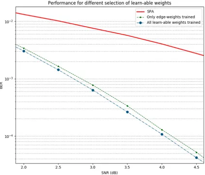
3.4 NND performance comparison of different hyper-parameter setting 34 3.5 Comparison for selection of learn-able weights . . . 36

3.6 Comparison of performance of NND for different number of SPA iterations. . . 38

3.7 Comparison of performance for different number of SPA iterations 39 3.8 Comparison for different network architectures . . . 40

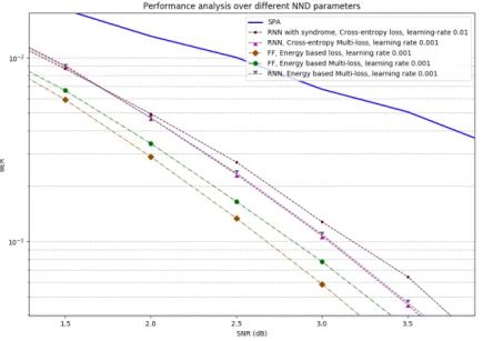
3.9 Comparison for syndrome check loss function . . . 44

3.10 Cross entropy vs Energy based loss function . . . 46

3.11 Comparison of different loss functions . . . 46

3.12 Comparison of SNR values for training (32,16) polar code. . . 49

3.13 Comparison of BER performance for different training epochs. . 50

4.1 Weight distribution analysis - (7,4) Hamming . . . 55

4.2 Weight distribution analysis - (7,4) tree . . . 56

4.3 Evolution of weights . . . 57 4.4 Decoding results and edge weight analysis for (32, 16) polar codes. 59 4.5 Decoding results and edge weight analysis for (32,24) polar code. 60 4.6 Decoding results and edge weight analysis for (128,64) polar code. 62 4.7 Decoding results and edge weight analysis for (63,45) BCH code. 64 4.8 Decoding results and edge weight analysis for (96,48) LDPC code. 65

(9)

List of Tables

3.1 Number of operations required to perform one SPA iteration in

NND. . . 31

3.2 Hyper-parameter list . . . 33

4.1 List of codes evaluated for their decoding performance with the NND. . . 56

4.2 Parameter settings for (32,16) polar code. . . 57

4.3 Parameter settings for (32,24) polar code. . . 58

4.4 Parameter settings for (128, 64) polar code. . . 61

4.5 Parameter settings for (63,45) BCH code. . . 61

(10)

Abbreviations

AWGN Additive White Gaussian Noise BCH Bose Chaudhuri Hocquenghem BER Bit Error Rate

BLER Block Error Rate BP Belief Propagation

BPSK Binary Phase Shift Keying DNN Deep Neural Network EML Energy based Multi-Loss FEC Forward Error Correction

FF-NND Feed Forward architecture based NND FFT Fast Fourier Transform

GF Galois Field

HDPC High Density Parity Check

i.i.d Independent and identically distributed IoT Internet of Things

KL Kullback-Leibler

LDPC Low Density Parity Check LLR Log Likelihood Ratio MAP Maximum a-Posteriori ML Maximum Likelihood

MPF Marginalization of Product Function NND Neural Network Decoder

NVS Normalized Validation Score

RNN-NND Recurrent Neural Network architecture based NND SPA Sum Product Algorithm

SPA-NN Sum Product Algorithm based Neural Network URLLC Ultra Reliable Low Latency Communication

(11)

Chapter 1

Introduction

1.1 Background

With an estimated 29 billion devices connected to the Internet by 2022 [15], the amount and diversity of the mobile communication will grow tremendously. 18 billion of those devices will be related to the Internet of Things (IoT), serving different use-cases such as connected cars, machines, meters, sensors etc. 5th

generation of communication systems are envisaged to support large number of IoT devices falling into the scenario of “Ultra Reliable Low Latency Commu-nication” (URLLC) with strict requirements on latency (within milliseconds) and reliability (Block Error Rate (BLER) < 10−5, and beyond). Forward Error Correction (FEC) codes are used for channel coding to make the communica-tion reliable. To ensure low-latency, the transmission data length has to be kept short, coupled with the low-complexity decoding algorithms.

1.1.1 Decoder Design

It has been 70 years since the publication of Claude Shannon’s celebrated A

Mathematical Theory of Communication [26], which founded the fields of

chan-nel coding, source coding, and information theory. Although Shannon theo-retically proved the existence of codes that can ensure reliable communication (up to a certain information rate below the channel capacity), he did not spec-ify methods or codes which can achieve this practically. Practically successful codes with high error-correcting capabilities must also have a low-complexity decoding algorithm to decode them. The decoding problem has no optimal polynomial time solution (NP-Hard), and for years researchers struggled to find an algorithm that achieves desirable performance with low complexity. A major breakthrough came with the introduction of iterative decoding algorithm, known as the Sum Product Algorithm (SPA) [13, 28], and re-discovery of Low Den-sity Parity Check (LDPC) codes, which performs near optimal with the SPA. However, the SPA performance remains sub-optimal for short length codes with good error-correcting capabilities as cycles are inherently present in the graphs of good codes (cf. Section 2.3.3). A short cycle in the graph degrades the per-formance of the SPA by forcing the decoder to operate locally so that the global optimal is impossible to find. In order to achieve near Maximum a-Posterior

(12)

(MAP) performance in decoding, the decoding algorithm must find the globally optimal solution in a cyclic code within the polynomial time complexity.

1.2 Problem Formulation and Method

In this thesis, we propose to develop methods to combine the expert knowledge of the systems, with data-driven approaches in machine learning, in an attempt to improve performance of the decoding algorithms. The scope of our study will be restricted to binary, symmetric and memory-less channels with Additive White Gaussian Noise (AWGN), and Binary Phase Shift Keying (BPSK) modulation in a single-carrier system. We restrict our study to binary linear block codes since they are the most commonly used codes in modern communication systems.

We will study different algorithms in the context of decoding linear block codes, and explore methods to incorporate data-driven learning using neural networks. In order to evaluate the performance of different algorithms, simula-tions will be carried out using various tools developed during this thesis.

The objectives of this thesis are: • Study and Investigate

– Graphical modeling and inference techniques, with focus on Factor graphs and message passing algorithms

– Data-driven machine learning techniques, with focus on the Deep Neural Networks (DNN) and its variants.

• Decoder design

– Study channel coding basics with focus on standard algorithms for decoding binary linear block codes.

– Review literature for methods using neural networks for decoding. Analyze methods for performance, scalability, and complexity. – Implement and analyze neural network based decoder algorithms that

improves upon the performance of standard SPA for short to medium length codes.

– Evaluate performance by comparing Bit-Error Rates (BER) and Block Error Rates (BLER) of different family of codes.

The aim of this thesis is not to design a complete receiver system, but to introduce methods that can enable data-driven learning in communication sys-tems, using already available expert knowledge about the system. Algorithms and analysis developed in this thesis are applicable to a wide variety of problems related to optimization of multi-variate systems.

1.3 Motivation

The primary motivation of this work came from (a) the recent advances in Machine Learning algorithms [18] and (b) the development of signal processing and digital communication algorithms as an instance of SPA on the factor graphs [20].

(13)

1.3.1 Neural Networks

Neural networks have long been applied to solve problems in digital commu-nications [19]. However, due to their high complexity in both training and application, they were mostly considered theoretically, and never applied in practice to the communication systems. More recently, due to advent of more powerful algorithms such as DNN, and tremendous increase in computational power of modern processors, there have been renewed efforts towards developing communication systems based on machine learning [8, 24]. Data-driven discrim-inative learning approach of DNN uses complex non-linear models to represent the system generating the data. Multi-layered feed-forward neural networks, such as the DNN, are a class of universal function approximators [16].

1.3.2 Graphical Modeling and Inference Algorithms

Communication systems are based on the probabilistic analysis of the underly-ing variables. These systems comprises of multiple variables (visible or hidden), and often we are interested in calculating the joint or marginal probability distri-bution of its variables. Graphical models provide an approach to augment this analysis using simplified graphical representation of the probability distribution of variables in the system [6]. Also, graphical modeling allows incorporating expert knowledge about relationships of the variables into the system model. Many algorithms deals with complicated systems of multiple variables by fac-torizing the global function (joint distribution) into product of local functions, which depends only on the subsets of the variables. Such factorization leads to reduced complexity, and provide an efficient methods (such as message passing algorithms) for making inferences about the variables.

A simple and general graphical construction to represent these factorizations is by using the Factor Graphs. Message passing algorithms operates on nodes of the factor graphs. When factor graphs are cycle-free, message passing algo-rithms provide exact inferences. However, for cyclic graphs, the inferences are approximate. For some problems the algorithm may converge to provide near-optimal results for cyclic graphs, but for other it will not. Decoding algorithm using the SPA is one instance of message passing algorithms on factor graphs.

In this work, we investigate methods to incorporate data-driven learning in the SPA decoder, in order to overcome some of its issues. The resemblance of the factor graphs with neural networks has motivated us to apply these two methods in conjunction.

1.4 Societal and Ethical Aspects

As our societies are moving towards greater connectivity and automation, the energy efficiency and sustainability of entire eco-systems becomes paramount. Communication systems are an essential part of any eco-system involving mul-tiple devices. In communication systems, improvements in the decoding perfor-mance of the receiver will lead to a reduction in the failed transmissions and re-transmissions, and hence, to a reduction in the overall energy consumption. Energy efficiency will help ensuring sustainability of IoT devices that are part of the massive machine-to-machine communication or URLLC framework. Ex-perimental results (see Chapter 4) shows that for short length HDPC codes, by

(14)

using the DNN based decoding algorithm, we can achieve a power gain of 2-4 dB compared to the standard SPA.

The DNN algorithms designed to model stochastic systems requires parallel training of the model on the actual online data in order to continuously adapt. Since devices usually possess minimal computational resources, online data is sent to a centralized system for processing. This may lead to ethical issues regarding privacy of the data. However, the linear block codes based coding system is a deterministic system. The DNN based algorithm for deterministic systems need not adapt to the online data. A DNN based decoder, trained sufficiently on artificially generated coding data, will provide the best decoding performance during its online run. Hence, the DNN based decoding algorithm may exempt from data privacy related ethical issues.

1.5 Thesis outline

In Chapter 2, we introduce concepts required to understand rest of thesis. The Neural Network Decoder (NND) design and analysis is presented in Chapter 3. Here, we also provide the previous related work in this field and present an in-depth analysis of hyper-parameters crucial to the performance and imple-mentation of the NND. In Chapter 4, we present experimental setup, analysis and decoding results for different families and sizes of codes. Finally, in Chapter 5, we present important conclusions drawn from the work, and give recommen-dations for the future research work.

1.6 Notations

In this section, we provide the basic notations that are used throughout this thesis. We follow the notations from set theory and coding theory. Note that some of the specific notations or symbols are introduced within the report as they are used.

An element x belonging to the set S is denoted by x ∈ S. A set S with

discrete elements will be specified by listing its elements in curly brackets, for exampleS = {1, 2, 3}. Size of a set is denoted by |S|. If a set S consists of only

those elements of another set X that satisfy a property F, then set S can be

denoted by S = {x ∈ X : F(x)}, or, if X is known, S = {x : F(x)}. Notations

such as union (∪), intersection (∩), subset (⊂), and their not operators (for

example /∈), have usual meaning from the set theory.

Operation⊗ denotes matrix cross product and ⊙ denotes matrix

element-wise product.

Consider, as an example, a set of multiple variablesX = {x1, x2, x3, x4}. The

operator backslash (\) between two sets of elements denotes exclusion of set of

elements on the right from the set on the left, for exampleS ={X \{x1, x2}

} =

{x3, x4}. The operator tilde (∼) before an element or set denote a set formed

by excluding the element, or set, from its parent set, for exampleS = {∼ x1} =

{

X \{x1}

}

={x2, x3, x4}. In such cases, parent set X must be known.

Sets are denoted by calligraphic capital letters, such asX . Bold type small

characters denote Vectors (x), and bold type capital letters denote Matrices (X). The ith element of a vector x is denoted by x(i), whereas (i, j)th element

(15)

of a matrix is denoted by X(i, j). Super-script and sub-script letters following a variable (XA,a

(16)

Chapter 2

Background

In this chapter, we provide the basics required to understand rest of the thesis work. We organize this chapter as follows. First, we present the basic com-munication system and channel model used in this study. Factor graphs and the Sum-Product Algorithm (SPA) are introduced next. Then we provide a brief overview of the coding theory and extend the SPA in context of decoding applications on the Tanner graph. We introduce neural networks in the last section.

2.1 Communication System Model

The goal of a communication system is to retrieve a message transmitted through a noisy communication channel. In the analysis of the decoder, we will use a simplified communication system model shown in Figure 2.1. The system is based on an AWGN channel and BPSK modulation. The encoded bits

si = {0, 1} are mapped to BPSK symbols yi = {+1, −1} †. The modulated signals, y ∈ {+1, −1}n_{, are transmitted through the AWGN channel, with} Gaussian distributed noise samples n ∼ N (0, σ2_{), σ} _{∈ R. Received signal is}

given by r = y + n. The signals received at the receiver are demodulated to give the likelihood of a symbols being transmitted. In an AWGN-BPSK communi-cation system, the received signal r is a Gaussian random variable with mean

µ ={−1, +1} and variance σ. Likelihood ratio is generally represented in log

domain, as Log-Likelihood Ratios (LLR), given by (2.1). These LLR values are fed into the decoder as input, and decoder attempts to correct each bit using the redundancy introduced in the code through the encoding process.

where ri is the received signal power (−1, 1) and σ is variance of the channel AWGN.

We make the following assumptions, (a) channel σ is real valued with power spectral density N0/2, and (b) transmitted symbols are independent and

iden-tically distributed (i.i.d).

†_{Notice that the modulation scheme maps}_{{0 → +1} and {1 → −1}, that is, y}

(17)

For the analysis of decoder, we use a BPSK modulation scheme in order to keep the complexity of the demodulator low, and focus only on the perfor-mance of the decoder. The assumption of AWGN channel is valid for decoder design because, in general, the communication system is designed ∗ _{such that}

the correlations induced by the channel are removed before sending information to the decoder. The performance of the SPA decoder degrades significantly for signals with correlated noise. Hence, it is important that the decoder receives i.i.d. information as input.

Source b : b ∈ {0, 1}k Encoder s = ξ(b) : s ∈ {0, 1}n_{, n > k} Modulator y = (−1)si Channel r = y + n : ni ∼ N (0, σn2) Demodulator PAWGN(si|ri) Decoder ˆ s = argmax s P (r|s) Sink ˆ b = ξ−1(ˆs)

Figure 2.1: Communication system model for decoder design.

2.2 Factor Graphs and Sum-Product Algorithm

In this section, we will introduce the factor graphs and the SPA as a general mes-sage passing algorithm to make inferences about the variables in factor graphs. Here, we develop the foundations for the work presented in this thesis. The in-troduction to factor graphs and SPA is also necessary to motivate the extension of this work to a wider range of problems. For a general review of graphical modeling and inference algorithms, we refer the reader to Chapter 8 of [6].

2.2.1 Generalized Distributive Law

Many algorithms utilize the way in which a complicated “global” function fac-torizes into the product of “local” functions. For example, forward/backward algorithm, the Viterbi algorithm, the Kalman filter, and the Fast Fourier Trans-form (FFT) algorithm. The general problem these algorithms are trying to solve can be stated as the “marginalization of a product function” (MPF). The MPF problem can be solved efficiently (exactly or approximately) using the

Gener-alized Distributive Law (GDL) [3] or SPA [20]. Both methods are essentially

the same, that is, they are based on the humble distributive law, that states

ab + ac = a(b + c). Let us take a simple example to show power of the

distribu-tive law.

∗_{Correlations in received information can be removed by scrambling the input bits before}

(18)

Example

Consider a function f that factorizes as follows:

f (x1, x2, x3, x4, x5) = f1(x1, x5) f2(x1, x4) f3(x2, x3, x4) f4(x4) (2.2)

where x1, x2, x3, x4, and x5 are variables taking values in a finite set A with q

elements.

Suppose that we want to compute the marginal function f (x1),

f (x1) = ∑ ∼x1 f (x1, x2, x3, x4, x5) =∑ x2 ∑ x3 ∑ x4 ∑ x5 f1(x1, x5) f2(x1, x4) f3(x2, x3, x4) f4(x4) | {z } marginal of products (2.3)

How many arithmetic operations are required for this task? For each of the

q values of x1 there are q4 terms in the sum defining f (x1), with each term

requiring one addition and three multiplications, so that the total number of arithmetic operations required are 4q5_.

We apply the distributive law to convert “marginal of products” into “prod-uct of marginals” as follows:

f (x1) = [ ∑ x5 f1(x1, x5) ][ ∑ x4 f2(x1, x4)f4(x4) ( ∑ x2,x3 f3(x2, x3, x4) )] | {z } product of marginals (2.4)

The number of arithmetic operations required to compute (2.4) are 2q2_+6q4_.

Moreover, if we wish to calculate other marginals, the intermediary terms in the product in (2.4) can be used directly, without re-computing them. If we follow the operations in (2.3), we will have to re-compute marginals for each variable separately, each requiring 4q5_{operations. For larger systems with many}

variables, the distributive law reduces the complexity of computing the MPF problem significantly.

The notion of “addition” and “multiplication” in GDL can be further gener-alized to operations over a commutative semi-ring [3]. Hence, the GDL holds for other commutative semi-rings which satisfy associative, commutative and dis-tributive laws over the elements and operations defined in the semi-ring, such as “max-product” or “min-sum”.

2.2.2 Factor Graphs

Factor graph provides a visual representation of the factorized structure of a system. They can be used to represent systems with complex inter-dependencies between its variables. A stochastic system can be modeled as the joint prob-ability of all its underlying variables, while systems with specific deterministic configuration of variables can be modeled using an identity function to specify the valid configurations. Factor graph are a straightforward generalization of the “Tanner graphs” [29]. The SPA operates on the factor graph to compute various marginal functions associated with the global function. The function

(19)

2.2a, or as a bipartite factor graph, as shown in Figure 2.2b. Notice that in a factor graph of a tree-structured system, starting from one node and following the connected edges, we can never reach the same node again.

x1 f1 x5 f2 x4 f4 f3 x2 x3

(a) Tree representation of function f .

f1 f2 f3 f4 x1 x2 x3 x4 x5

(b) Bipartite graph representation of f .

Figure 2.2: Graphical representation of function f in (2.2).

2.2.3 Sum-Product Algorithm

The SPA operates by passing messages over the edges of the factor graph. For tree-structured graphs, such as the one shown in Figure 2.2a, the SPA gives exact inferences, while for graphs with cycles, the inferences made by the SPA are ap-proximate. The basic operations in SPA can be defined using just two equations - variable to local function message (µx_→f given by (2.5)), and local function to variable message (µf_→x given by (2.6)). Variable to local function:

µx→f(x) = ∏ h_∈n(x)\{f}

µh→x(x) (2.5)

Local function to variable:

µf→x(x) = ∑ ∼{x} ( f (X) ∏ y∈n(f)\{x} µy→f(y) ) (2.6)

where n(x) denotes the neighboring elements of x in the bipartite graph. For example, n(x1) ={f1, f2} and n(f2) ={x1, x4}.

We will explain the SPA by solving the MPF problem given by (2.4), by message passing over the corresponding tree-structured graph shown in Figure 2.2a. The idea is to compute the marginal f (x1) by passing messages along

the edges of the graph, and applying two basic SPA operations alternatively till all nodes are covered. We start the computations at the leaf factor nodes with least number of variables, that is f3 and f5. The messages reaching an

intermediate variable node (for example x4) should only be a function of that

variable, with other variables being marginalized out of the message before reaching this node. The function f3is marginalized out of the variables x2 and

(20)

x3using (2.6), sending the message µf3→x4(x4) towards node x4. This step gives

us the rightmost element in the product in (2.4), that is ∑_x₂_,x₃f3(x2, x3, x4).

A node must receive information from all the connected edges, except the edge connecting the parent node, before it can send information to the parent node. Hence, variable node x4 has to receive message µf4→x4(x4) from node f4before

sending a message to node x1.

Now, once node x4 has received information from its connected edges, it

calculates the message µx4→f2(x4) =

∏

µf3→x4(x4)µf4→x4(x4) using (2.5) and

send it to node f2. The factor node f2passes message µf2→x1(x1) by

marginal-izing out the variable x4, using (2.6). Similarly, variable node x1 receives

mes-sage µf 1→x1(x1) from f1 by marginalizing out variable x5. The two messages

reaching variable node x1 represent the two multiplying factors in (2.4). The

marginal of f (x1) is obtained by taking product of these two messages reaching

node x1. Hence, we see that the SPA is essentially applying equations (2.6) and

(2.5) alternatively, starting from the leaf nodes, till we reach the root node. By applying these equations to the entire graph, one can calculate the marginals of all variables.

Now consider the SPA operations over the factor graph of the same problem shown in Figure 2.2b. The variable nodes xi initialize messages µxi→fj(xi) as

some constant value or as observed values from the system. The factor nodes

fjapply (2.6) to calculate the messages that are passed back to variable nodes. Next, the variable nodes apply (2.6) to calculate new messages to send forward to factor nodes. Notice that a factor node fj (or variable node xi, respectively) calculates the message µfj→xk(xk) (or, µxi→fk(xi)) using incoming information

from all variable nodes connected to fj (or xi), except the variable node xk (or fk) to which it will send this information forward. If variable nodes have initial observations, these observations are added to the variable node’s outgoing messages. The variable and factor nodes process information iteratively in this fashion, until there are no more nodes remaining to pass the information (in case of tree-structure), or time runs out (in case of cyclic structures). The application of the SPA on graph with cycles leads to an approximate inference of the variables. We will come back with some more details on the SPA for Tanner graphs with cycles in Section 2.3.2.

2.3 Coding Theory

A linear block code, denoted byC(n, k), is a code of length n which introduces redundancy in a block of k information bits, by adding n− k parity check bits that are functions (”sums” and ”products”) of the code and the information bits. A block code is linear if its codewords form a vector space over the Galois Field GF(q), that is any linear combination of the codewords is also a codeword. In this thesis, we consider binary codes restricted to the field GF(2), consisting of the set of binary elements {0, 1} with modulo-2 arithmetic. Note that an

all-zero codeword is a member of any linear block code since adding an all-zero codeword to any other codeword will give the same codeword (identity prop-erty). The encoding process can be explained as a vector-matrix multiplication of the information bits vector with a Generator matrix G of size [n, k], that is

y = G⊗ b. The rows of a Generator matrix forms the basis of the linear-space

(21)

[n, n− k], which possesses the property GT_{⊗ H = 0.} The rate of the code is defined by r = k

n, that is number of information bits per transmitted bit. The Hamming distance between two codewords is defined as the number of positions where bit values are different in both code-words. In terms of GF(2) arithmetic, dh = y− x, y, x ∈ C. The Hamming weight of a codeword is defined as the Hamming distance of the codeword with the all-zero codeword. The minimum distance of a code is defined as

dmin = mindhdh(y, x)∀y, x ∈ C, or as minimum Hamming weight within all

codewords in the code-book.

2.3.1 Maximum Likelihood Decoding

The task of the decoder is to find the transmitted codeword s, given the received signal r. An optimal decoder will choose the codeword (ˆs ∈ C) which gives the maximum probability for the received signal p(r|s). This is the Maximum

Likelihood (ML) decoder. ˆ

s = argmax s:s_∈C

p(r|s) _(2.7)

In order to find a ML decoding solution, one has to look into the entire set of 2n _{possible codewords to find the one which gives the maximum probability} of the received signal being r and satisfies the parity check HT _{⊗ s}T _{= 0}T_. This problem becomes prohibitively complex as the length of the codeword becomes longer. In fact, ML decoding problem has no polynomial time solution (see section 1.7.3 in [25]). Hence, it is reasonable to look for some heuristic solutions, including neural networks.

2.3.2 Iterative Decoder Design

The iterative decoder is based on the SPA, which operates by passing messages over the Tanner graph of the code. Let us first give a brief review of the Tanner graph representation of a linear block code.

Tanner Graph representation of code

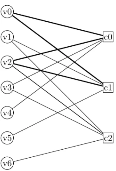
The Tanner graph is a bipartite graph that represents the linear constraints present in the codeC(n, k). Any codeword must satisfy the parity check

condi-tion HT_{⊗ s}T _{= 0}T_{. Using this property of the parity check matrix, the Tanner} graph can be constructed by representing the columns of parity check matrix as the variable nodes v, and the rows as the check nodes c. An edge connects the variable node vj to check node ci if there is a “1”, instead of “0”, at (i, j) position in H. Any binary vector y = {0, 1}n _{will be a codeword of the code}

C(n, k) if it satisfies every check defined by the modulo-2 sum of values of the

variable nodes connected to the corresponding check nodes.

For example, consider [7,4] hamming code with parity check matrix H given by, H =  11 01 11 10 10 01 00 0 1 1 1 0 0 1   (2.8)

(22)

The tanner graph given by this matrix is shown in Figure 2.3. Notice the configuration of the edges connecting two sets of nodes in the Tanner graph, and “1”s in the parity check matrix.

c0 c1 c2 v0 v1 v2 v3 v4 v5 v6

Figure 2.3: Tanner graph of the parity check matrix of (7,4) Hamming code.

Decoding using Sum Product Algorithm

The SPA introduced in Section 2.2.3 is the general message passing algorithm for making inferences on the factor graphs. Now, we will look at the SPA for the special case of decoding on the Tanner graphs. We will see that the exact formulation will be greatly simplified for the case of binary variable systems.

For binary variable case, we can think of the messages µf_→x and µx_→f as real-valued vectors of length 2, given by{µ(1), µ(−1)}. The initial message for

a variable node xi is the probability of the bit received at the ith realization of the channel, given by µ(xi) = {p(ri|xi = 1), p(ri|xi =−1)}. Recall that for a variable node, the outgoing message take the form (2.5),

µx→f(1) = ∏ k µfk→x(1) µx→f(−1) = ∏ k µfk→x(−1) (2.9)

Let us consider the check node messages. The check f nodes sends message to a variable node x about its belief that the variable node is +1 or−1.

µf_→x(x) ={ µf_→x(1), µf_→x(−1) } ={ ∑ ∼x f (1, x1, . . . , xJ) ∏ j µj(xj), ∑ ∼x f (−1, x1, . . . , xJ) ∏ j µj(xj) } (2.10) We introduce LLR using (2.1) to obtain a single value denoted by l = ln_µ(µ(1)₋₁₎. Furthermore, the check node function can be written as an indica-tor function whose value is 1 if the parity check is satisfied, 0 otherwise, that is

(23)

f (x, x1, . . . , xJ) =I( ∏

jxj = x). Notice that since the symbols x∈ {1, −1} we can write ∏_jxj = x instead of

∑

jxj = x. The outgoing message at a check node is given by equation 2.6. The message in (2.10) can be written as

lf_→x= ln ∑ ∼xf (1, x1, . . . , xJ) ∏ jµj(xj) ∑ ∼xf (−1, x1, . . . , xJ) ∏ jµj(xj) e(lf→x)₌ ∑ x1,...,xJ:∏jxj=1 ∏ j µj(xj) µj(−1) ∑ x1,...,xJ:∏jxj=−1 ∏ j µj(xj) µj(−1) = ∑ x1,...,xJ:∏jxj=1 ∏ je (lj(1+xj)/2) ∑ x1,...,xJ:∏jxj=−1 ∏ je(lj(1+xj)/2) = ∏ j(e lj _{+ 1) +}∏ j(e lj − 1) ∏ j(elj + 1)− ∏ j(elj − 1) = 1 +∏_j elj−1 elj+1 1−∏_j elj−1 elj+1 (2.11)

The last two steps follows as we expand out ∏_j(elj _{+ 1) and} ∏

j(e

lj − 1) for

xj= 1 and xj=−1 for numerator and denominator, respectively. Using the function tanh(lj/2) = e

lj₋₁

elj+1, we get a simplified form given by,

lf→x= 2 tanh−1 ( ∏ j tanh(lj/2) ) (2.12) Similarly, the outgoing message by a variable node is given by standard SPA equation (2.5), can be written in context of decoding as,

lxi→fj = ln ∏ k µfk→xi(1) µfk→xi(−1) =∑ k lk (2.13)

where the summation is over k factor nodes connected to the variable node xi, except the factor node fj.

The final output LLR is calculated by adding the channel information to all messages received by the variable node after one iteration.

l∗k = lk+ ∑

i

lfi→xk (2.14)

Hence, we got two simplified equations for messages µx→f (2.13), and µf→x (2.12). The general flow of SPA is given in Algorithm 2.1.

2.3.3 Cycles and trapping sets

The SPA works optimally for the Tanner graphs that forms a tree structure, in which the variable relationships can be factored exactly, leading to optimal solution of the MPF problem through iterative message-passing. However, the codes represented by graphs with no-cycles have low minimum distance, and hence perform poorly. This can be explained through the following argument (see section 2.6 in [25]).

(24)

Algorithm 2.1 SPA algorithm Initialize: lj= LLRj lxj→fi= lj c = 0, C = max iterations repeat c = c + 1 Parity Check ˆ sk= { 0, l∗_k > 0 1, otherwise if ˆs⊗ H = 0 then Estimated codeword = ˆs END end if lfi→xk= 2 tanh −1( ∏ j\ktanh(lxj→fi/2) ) lxk→fi= ∑ j\ilfj→xk l∗_k= lk+ ∑ ilfi→xk until END or c = C

Lemma†_{: A binary linear code C, with rate r and the Tanner graph forming}

a tree, contains at least 2r₋₁

2 n codewords of hamming weight 2.

Proof†_{: The graph of C contains n variable nodes (corresponding to each bit}

of encoded information), and (1−r)n check nodes. Total number of nodes in the

tree are 2n−nr. Hence average number of edges connected to each variable node

is upper bounded by 2− r. Each internal variable node (variable node that are

not leaf nodes) has degree at least 2. It follows that the number of leaf variable nodes x must be greater than nr (proof: x+2(n−x) ≤ 2n−nr ⇒ x ≥ nr). Since

every leaf variable node is connected to only one check node, we have at least

rn− (1 − r)n = (2r − 1)n leaf variable nodes that are connected to check nodes

with multiple adjacent variable nodes. Each of these (2r− 1)n leaf variable

nodes has a pair of another leaf variable node, which give rise to a codeword of weight 2 for rates above one-half. Even for codes with rate less than one-half, tree structured Tanner graph based codes contain low-weight codewords.

It has been observed that the SPA performance degrades due to two major artifacts of the code or Tanner graphs. One is the minimum distance of the code, and other is the Trapping sets or Stopping sets in the Tanner graph. A trapping setT is a subset of variable nodes V such that all neighbors of T , that

is, all check nodes connected toT , are connected to T at least twice. A cycle is

a trapping set, but opposite is not always true. Trapping sets leads to situations from which SPA fails to recover. An example of cycle and trapping set is shown in figure 2.4.

(25)

c0 c1 c2 v0 v1 v2 v3 v4 v5 v6

Figure 2.4: The cycles are marked with thick edges in the figure. Also variable nodes{v0, v1, v2} form a trapping set with check nodes {c0, c1, c2}.

2.4 Neural Networks

In this section, we introduce some of the basic concepts of Neural Networks required to understand rest of the thesis. For a more comprehensive text, we refer the reader to the book on deep learning by Ian Goodfellow [18].

2.4.1 Introduction

The basic idea behind supervised machine learning techniques is to learn a func-tion f modeled using a parameter set w to represent the system generating the target data x. Consider a model represented by a function of non-linear activa-tions and basis funcactiva-tions. In machine learning terminology, this model is called a Linear Regression model, which perform well for regression or classification problems. f (x, w) = α (N∑−1 i=0 wiϕi(x) ) = α ( wTϕ(x) ) (2.15) where ϕi() are non-linear basis functions and α() is a non-linear activation func-tion.

The machine learning algorithms perform regression or classification tasks by learning the model parameters w during the training phase. The training phase essentially provides the model with some experience (data) to transform itself in order to resemble the actual data generating system. The neural networks use the same form as (2.15), but each basis function in-turn becomes a non-linear function of the linear combinations of inputs. Hence the basic neural network model can be described by a series of linear and non-linear transformations of the input.

Figure 2.5 shows a simple fully-connected feed-forward neural network. The input x is fed into the model through the input layer, which have same number of nodes as |x|. At the first hidden layer, we introduce first set of learn-able

(26)

parameters† _w(1)_{. The output of the first hidden layer is obtained by applying}

a non-linear activation function α1(·) on the linear combinations of the input.

Notice that the basis function for the input layer is ϕi(x) = xi. This output is again transformed in the second hidden layer by another set of learn-able parameters w(2) _{and a non-linear activation function α}

2(·). Finally, we obtain

the output y at the last layer using a last set of transformations. The training data must contain the pair of input and output (x, y) values that are used to train the parameters w(1)_{, w}(2)_{, w}(3)_{. The number of nodes in the input and}

output layers are fixed, but the number of hidden layers and the number of nodes in each hidden layer are hyper-parameters of the model, that can be set to any value based on the complexity of the system. Similarly, the non-linear activation functions are another set of hyper-parameters. As the number of hidden layers increases, and the network becomes deeper, the neural network model becomes capable of representing a highly complex and non-linear system. Similar effect is seen as the number of hidden nodes in the network are increased. However, as the complexity of the model grows, the number of learn-able parameters will increase, and therefore training process will require more training data to find the optimal values for these parameters.

Activation functions

The role of activation function in the neural networks is to introduce some non-linearity in the model, and to obtain the output of the network in some desired range of values. In general, activation functions must be continuous (smooth with finite first order derivatives) and finite valued for entire range of inputs. For a list and description of most general activation functions, refer to Section 6.3.3 of [18]. However, in our implementation we will use tanh−1 activation, which leads to exploding values of the output as the input reaches ±1. The problem of exploding values and gradients can be circumvented by clipping the function’s output in finite range. The derivative in that case will be clipped to match the clipped output value as well.

2.4.2 Network Training

The aim of the training process is to find the optimal values of the learn-able parameters w, such that the the error in estimation or classification is minimized during the online phase‡ _{of the model. However, since the model is trained to}

minimize the errors in estimating the training data, the estimation errors during the online phase may not see the same, and hence one has to validate the trained model separately to qualify a model for desired online performance. The online data used for validation is called the validation data. The function designed to quantify the models performance during training is called loss function . The ML estimator is commonly used to evaluate a loss function in the system.

†_{A learn-able parameter is a variable subjected to adjustments during the training process.} ‡_{The online phase of a model refers to its operation on the trained model using the input}

(27)

Layers (k)→ Output o(k) i → input (0) ϕi(x) = xi hidden (1) α(1)( ∑ iw (1) i o (0) i ) hidden (2) α(2)( ∑ iw (2) i o (1) i ) output (3) α(3)( ∑ iw (3) i o (2) i )

Figure 2.5: A fully-connected neural network with 2 hidden layers. Loss function

The optimal parameters for a neural network are the ones that minimizes a loss function L(x, y = f (x, w)). The loss function is an optimization problem that is usually written as,

wopt= argmax w

pmodel(x, y = f (x, w)) (2.16)

The exact formulation for the loss function depends on the system and the problem. We will discuss loss functions specific to the problems tackled in this thesis in Section 3.3.6. The loss function is fundamental to the performance of a neural network. An ill-formed loss function will lead to poor performance, even if the network learns the optimal parameters for the given training data. Regularization

Regularization helps keeping neural network from over-fitting. Different meth-ods and techniques can lead to regularization effect on the network’s parameters. Most significant are the weight regularization and early stopping.

Weight regularization puts constraints on the value of the learn-able param-eters by adding L− p norm of all parameters to the network’s loss function.

Most common form is the L− 2 norm, which puts a constraint on the weights

to keep norm of the parameter values close to 1. Early Stopping Criteria

Early stopping is often necessary to keep the network from deviating from the optimal values. We use Algorithm 2.2 for early stopping of the training process.

(28)

The algorithm let the network train for n epochs before validating its perfor-mance on a validation data-set. If the validation score of current validation test is better than all other test previously, then we save the weights at current state of the network. Once the network reaches its best performance, the validation scores will start to worsen. We observe the validation scores for at least p next validation tests, that is p× n training epochs, to find a better score. If not,

we stop the training and return the weights that gave the best validation score recorded.

Algorithm 2.2 Early Stopping Algorithm

n = number of training epochs before validation run.

p = number of validations to observe worsening validation score before giving

up.

θ0 = initial learn-able parameters.

Initialize θ← θ0, i← 0, j← 0, v← ∞, θ⋆_{← θ,} i∗ ← i while j < p do

Conduct training for n epochs, update θ

i← i + n v′← ValidationScore(θ) if v′< v then j← 0 θ⋆_{← θ} i∗ ← i v← v′ else j← j + 1 end if end while

θ⋆ _{are the best parameters, training ended at epoch i}_{∗ with validation score}

v.

2.4.3 Parameter Optimization

After designing the loss function and training process, we move to the task of solving the optimization problem, and finding the optimal weights w that minimizes the designed loss function L(w). Changing the weights w by a small amount δw leads to a change in loss function given by δL≃ δwT_{∇L(w). The} vector∇L(w) points towards the direction of greatest rate of change of the loss

function. Assuming that the designed loss function is a continuous and smooth function of w, its minimum∗ _{will occur at a point where} _{∇L(w) = 0. Due to}

∗_{Zero gradient is obtained at points corresponding to all minimum, maximum or}

saddle-point solutions. We apply stochastic gradient descent method to find the global minimum solution.

(29)

non-linearity of the loss function with respect to weights, and a large number of points in the weight-space, the solution to ∇L(w) = 0 is not straight forward. Most common method for optimization is neural networks is the Stochastic

gradient descent method. The gradient of the loss function with respect to a

parameter is calculated using the back-propagation method. Then the weights are updated towards the negative direction of the gradient.

Back-Propagation

The back-propagation method, or simply backprop, provides an efficient tech-nique for evaluating gradients of the loss function in neural networks. The loss function is a function of parameters w. The backprop method is based on the chain rule of derivatives. For the network shown in Figure 2.5, consider that the non-linear function as ϕi(x) = x. The partial derivative of loss function corresponding to the nth training data with respect to the ith parameter of the

jth hidden layer w_i(j)is given by

δLn δw_i(j) = δLn δo(j)_i δo(j)_i δw_i(j)

The second partial derivative term will simply be equal to the output of the previous layer o(j_i −1) (since ϕi(x) = x). The first term can be calculated by applying the chain rule again.

δLn δo(j)_i =∑ k δLn δo(j+1)_k δo(j+1)_k δoj_i

where the sum runs over all units k in layer j + 1 which unit i in layer j sends the connection. The chain rule is applied till we reach the last layer, where we calculate the gradient of the loss function with respect to the output of the last layer. Only this last partial derivative term depends on the design specific to the loss function. However, since we are propagating the errors backwards, the design of the loss function have significant effect on the gradients for all parameters.

The final gradient is calculated as a sum of gradients over a set of training data, given by equation 2.17. The Stochastic gradient descent method samples randomly from a subset of the training data to accumulate the gradients. The new weight is calculated by shifting the old value towards negative direction of the gradient, given by equation 2.18. The hyper-parameter η is called the learning rate of the optimization process. This parameter is adaptively adjusted to enable the gradient descent algorithm to slowly move towards the optimal minimum point. We use RMSProp optimizer for adaptive learning [18].

δL δw_i(j) =∑ n δLn δw(j)_i (2.17) w = w0− η ∑ n δLn δw (2.18)

(30)

2.4.4 Online Phase

The online or test phase of the neural networks is when we operate the trained neural network model using the inputs from the real data generating system. In online phase, the learned parameters of the network are fixed to their optimal trained values. The outputs are generated using this model by applying the neural network model on the online input data. Since there is no learning during this operation, the computations in online phase are only limited to the forward pass of the information in the model. During validation, we perform similar operations as the online phase. However, in order to validate the performance, the validation data contains pair of both input and output, which is used to calculate the validation scores.

(31)

Chapter 3

Neural Network Decoders

Linear block codes provide an efficient representation of information by adding parity checks for error correction. The decoder solves the linear optimization problem that arises due to the correlations present in the encoded data. Opti-mal Maximum Likelihood (ML) decoding of linear block codes can be classified as an NP-Hard problem (see Section 1.7.3 in [25], or [5]), and therefore it is reasonable to consider sub-optimal polynomial time solutions, including the neural networks. In this chapter, we will introduce a method to incorporate data-augmented learning to the problem of decoding linear block codes. The restriction to binary codes comes from the fact that the Neural Network Decoder (NND) is built using operations from the iterative decoder (cf. Section 2.3.2), where messages are the Log-Likelihood Ratios (LLR) of binary variables. The NND algorithm can be applied to solve a set of optimization problems similar to the decoding problem, that involves optimization of a linear objective func-tion in a constrained system of binary variables. The optimal solufunc-tion to these problems is obtained by marginalizing out all variables except the desired vari-able in the system. Different algorithms, such as the Belief Propagation (BP) [25] or Linear Programming Relaxation [11], have been proposed to find a poly-nomial time solution to the NP-Hard problem of decoding. These algorithms can be represented over the factor graphs, and solved using message passing algorithms such as the Sum Product Algorithm (SPA) [20]. The NND enables data-augmented learning over the factor graph of linear block codes (the Tanner graph) and implements the SPA for a system of binary variables.

Neural networks have been very successful in the representation learning of non-linear data [4]. In [7], authors presented ways of relating decoding of error correcting codes to a neural network. Many neural network designs and algorithms for decoding emerged later on, such as feed-forward neural networks [9], Hopfield networks [10], Random neural networks [2], etc. Although these algorithms perform better than the standard SPA, they failed to scale with the length of the code. Even after the recent growth in the performance of neu-ral network algorithms and the computational power of the modern processors, scalability of these algorithms remains as a bottleneck [12]. This curse of dimen-sionality is due to the fact that the number of possible words grows exponentially with the length of the code (n :C(n, k)). A decoder must learn to map all 2n possible words to 2k _{possible codewords. The neural network decoder has to be} trained on a large proportion of the entire code-book for achieving satisfactory

(32)

results [12]. For example, in case of a codeC(50, 25), the total possible words 250_{∼ 10}15 _{has to be mapped to total possible codewords 2}25_{∼ 10}7_{. Moreover,}

the size of the neural network will also grow with the length of the code, adding to the complexity of algorithms.

Recently authors of [22] presented a neural network based decoding algo-rithm that is based on the iterative decoding algoalgo-rithm, the SPA. The neural network is designed as an “unrolled” version of the Tanner graph to perform the SPA over a fixed graph. Hence, the neural network used in this algorithm inher-its the structural properties of the code, and algorithmic properties (symmetry, etc.) of the SPA. It shows significant improvements over the SPA by learning to alleviate the effects of artifacts of the Tanner graph such as cycles or trapping sets.

Our contributions in this thesis work are as follows:

– Analysis of various parameters affecting the training and online perfor-mance of the NND algorithm. The plethora of parameters considered in this work will also provide insights into the hyper-parameter selection for similar neural network algorithms, designed in the context of wireless communications.

– Introduction of a new loss function for training the NND that improves the performance compared to standard cross-entropy based loss functions. The new function bolster the model towards correct predictions where the SPA shows uncertainty, but prevents pinning of parameters to extreme values due to the strong SPA predictions, which are generally correct. – Analysis of weights distribution of the trained NND and deeper insight

into working of the NND based on this distribution. We extend the anal-ysis provided by [22] by looking into the evolution of weights in different iterations, and compare different architectures.

– Analysis of NND’s performance on different families and sizes of linear block codes, such as Hamming, BCH, polar, and LDPC codes.

The rest of this chapter is organized as follows. In the next section, we will revisit the SPA in order to define its graph and operations over the unrolled version of the Tanner graph. Next, we provide a description of the NND’s architecture and operations. Further, we present an analysis of the NND’s hyper-parameters related to design, optimization and training, as well as their optimal selection process.

3.1 Sum-Product Algorithm revisited

In this section, we will provide an alternative representation for the Tanner graph and the SPA, previously introduced in section 2.3.2. This new represen-tation, called the SPA over Neural Networks (SPA-NN), provides a method to implement the SPA operations (eq. 2.13, 2.12) using the neural networks. The SPA involves iterating messages forward and backward over nodes of the Tanner graph. In SPA-NN, the neural network nodes will correspond to the edges of the Tanner graph on which the SPA messages are being transmitted. Figure 3.1

(33)

shows the SPA-NN graph and an unrolled version of the Tanner graph for the (7,4) Hamming code corresponding to two full SPA iterations.

Consider L iterations of the SPA. Each iteration corresponds to passing the SPA messages twice (once in each direction) over the corresponding edges of the Tanner graph. This can be equivalently represented by unrolling the Tanner graph 2L times, as shown in Figure 3.1b. One of the drawbacks of SPA-NN is that it is designed for a fixed number of iteration, whereas SPA can be operated for any number of iterations till the satisfactory results are found.

The hidden layers in the SPA-NN graph are indexed by i = 1, 2, . . . , 2L, and the input and the final output layers, by i = 0 and i = 2L + 1, respectively. We will refer to the hidden layers corresponding to i = {1, 3, 5, . . . , 2L − 1}

and i = {2, 4, 6, . . . , 2L} as odd and even layers, respectively. The number of

processing nodes in each hidden layer is equal to the number of edges in the Tanner graph, indexed by e = (v, c) : e ∈ E. Each hidden layer node in this

graph calculates a SPA message transmitted in either one of the two directions over an edge of the Tanner graph. An odd (or even, respectively) hidden layer node e = (v, c), computes the SPA message passing through the edge connecting the variable node v (check node c, respectively) to the check node c (variable node v, respectively). Final marginalized LLR values can be obtained after every even layer. The channel information (initial LLR values) at the decoder input, are represented by lv, and the updated LLR information, received at an edge e of any even layer, are denoted by le. Each set of “odd-even-output” layers correspond to one full iteration of the SPA in the SPA-NN graph. Figure 3.1b shows how the edges in either directions in the unrolled version of the Tanner graph (shown as red and blue edges) are translated to a hidden layer node in the SPA-NN in Figure 3.1a. The neural network architecture and operations translating the Tanner graph based SPA into the SPA-NN, are described in the following sections.

3.1.1 Network Architecture

The connections between different layers in the SPA-NN graph can be under-stood by following the flow of information over the edges of the unrolled Tanner graph. We will use Figure 3.1 as an example to get a better understanding of this message flow and the architecture of the SPA-NN graph.

Let us consider the Tanner graph based SPA as described in Section 2.3.2. A single SPA iteration entails passing of information from (a) variable node to check node (red edges), (b) check node to variable node (blue edges), and (c) final output at the output node (green node and edges). The extrinsic information obtained at variable nodes in step (b) is passed on to perform the next iteration. Figure 3.1b converts the forward and backward information flow in the Tanner graph to a single direction of information flow in an unrolled graph.

Now consider the SPA-NN graph as shown in Figure 3.1a. The initial channel information is inserted into the network at the input layer nodes (i = 0). A node in the first hidden layer of the SPA-NN (red node in Figure 3.1a) indexed as

e = (v, c), represents an edge in the Tanner graph (red edge in Figure 3.1b) that

sends channel information from the input nodes associated with variable node

v, towards the check node c. Notice that any node in the first hidden layer of

(34)

(a) Network graph of the SPA-NN with nodes as edges of Tanner graph. v0 v1 v2 v3 v4 v5 v6 c0 c1 c2 v0 v1 v2 v3 v4 v5 v6 c0 c1 c2 L1 v0 v1 v2 v3 v4 v5 v6 L2

(b) Unrolled Tanner graph and the SPA message flow for two full iteration.

Figure 3.1: The SPA-NN and the Tanner graph for (7,4) Hamming code rep-resenting two full iteration of the SPA. In Figure (a), red (blue, respectively) nodes corresponds to odd (even) hidden layers in the SPA-NN. The output layer nodes are ingreen. The Tanner graph, shown in Figure (b), is the unrolled ver-sion for two SPA iterations. The information is flowing from left to right in both graphs. The SPA message flow, leading to the output LLR of variable v0

in the Tanner graph, is shown by dashed lines in Figure (b). The nodes in the SPA-NN corresponding to the dashed edges in the Tanner graph in Figure (b), are shown by bold circles in Figure (a).

(35)

SPA-NN (blue nodes in Figure 3.1a) represents passage of extrinsic information

le corresponding to the edges connecting check nodes to variable nodes (blue edges in Figure 3.1b). That is, every even layer node e = (v, c) is connected to the nodes of previous odd layer i− 1 associated with the edge e = (v′_{, c)} for v ̸= v′ _{(cf. eq. 2.12). After every iteration in the Tanner graph, we obtain} the final output for that iteration by adding the channel information lv to the updated LLR information lereceived from all check nodes (cf. eq. 2.14). This operation is performed after every even layer node, at the output layers of the SPA-NN (green nodes in Figure 3.1a). The number of output layer nodes is equal to the number of variable nodes in the Tanner graph. An output layer node receives extrinsic information lefrom the previous corresponding even layer nodes, and the channel information lv from the input layer nodes. Hence, each output layer node, indexed by v, has two connections, one to the previous even layer nodes and another to the input layer nodes. Notice that the output layers receive extrinsic information lefrom all edges connected to the variable node v, without exception. Note that the green line in Figure 3.1b represents the green nodes in Figure 3.1a.

In subsequent iterations of the SPA from the second iteration onwards, the variable nodes forwards a sum of the information it received from (a) the cor-responding check nodes (except the message it sent to the check node in the previous step) and (b) the channel information (cf. eq. 2.13). Similarly in the SPA-NN, odd hidden layer nodes (e = (v, c)) corresponding to second iteration onwards (i > 2), receives extrinsic information (le) from the previous even layer (i− 1) associated with the edge e = (v, c′_{) for c}_{̸= c}′_{, as well as channel} infor-mation (lv) from the input layer. Note that the channel information input to any odd layer is shown by small black rectangular boxes in Figure 3.1a. Design Parameters

The architectural design of the SPA-NN can be represented using a set of config-uration matrices. These matrices will define the connections between different layers in the neural network of the SPA-NN. The compact matrix description of the neural network architecture will help in formulation of SPA-NN entirely us-ing the matrix operations.

Notations:

We will use following notations to define different sets of nodes in the graph:

V = Set of all variable nodes in Tanner graph of C G = Set of all check nodes in Tanner graph of C E = Set of all edges in Tanner graph of C

Φ(e) = {v ∈ V : ∃ e = (v, c) ∀c ∈ G, e ⊂ E} = Set of all variable nodes con-nected to a set of edges given by e.

Σ(e) ={c ∈ G : ∃ e = (v, c) ∀v ∈ V, e ⊂ E} = Set of all check nodes connected to a set of edges given by e.

Network layer sizes:

The sizes of network layers are defined as follows:

Input layer size = Output layer size = no. of variable nodes = n Hidden (odd, even) layer size = no. of 1s in H = no= ne=

∑

Machine Intelligence in Decoding of Forward Error Correction Codes

IN

DEGREE PROJECT

INFORMATION AND COMMUNICATION

TECHNOLOGY,

SECOND CYCLE, 30 CREDITS

,

STOCKHOLM SWEDEN 2017

Machine Intelligence in Decoding

of Forward Error Correction Codes.

NAVNEET AGRAWAL

Abstract

Sammanfattning

Acknowledgment

Contents

List of Figures

List of Tables

Abbreviations

Chapter 1

Introduction

1.1 Background

1.1.1

Decoder Design

1.2

Problem Formulation and Method

1.3

Motivation

1.3.1

Neural Networks

1.3.2

Graphical Modeling and Inference Algorithms

1.4

Societal and Ethical Aspects

1.5 Thesis outline

1.6

Notations

Chapter 2

Background

2.1

Communication System Model

2.2

Factor Graphs and Sum-Product Algorithm

2.2.1

Generalized Distributive Law

2.2.2

Factor Graphs

2.2.3

Sum-Product Algorithm

2.3

Coding Theory

2.3.1

Maximum Likelihood Decoding

2.3.2

Iterative Decoder Design

2.3.3

Cycles and trapping sets

2.4

Neural Networks

2.4.1

Introduction

2.4.2

Network Training

2.4.3

Parameter Optimization

2.4.4

Online Phase

Chapter 3

Neural Network Decoders

3.1

Sum-Product Algorithm revisited

3.1.1

Network Architecture