Full Terms & Conditions of access and use can be found at
https://www.tandfonline.com/action/journalInformation?journalCode=clah20
Labor History
ISSN: (Print) (Online) Journal homepage: https://www.tandfonline.com/loi/clah20
The wage share and government job creation in
Sweden, 1900–2016
Lars Ahnland
To cite this article: Lars Ahnland (2020) The wage share and government job creation in Sweden,
1900–2016, Labor History, 61:3-4, 228-246, DOI: 10.1080/0023656X.2020.1731732 To link to this article: https://doi.org/10.1080/0023656X.2020.1731732
© 2020 The Author(s). Published by Informa UK Limited, trading as Taylor & Francis Group.
Published online: 25 Feb 2020.
Submit your article to this journal
Article views: 1157
View related articles
The wage share and government job creation in Sweden,
1900
–2016
Lars Ahnland
Ekonomisk historiska institutionen, Stockholm University, Stockholm, Sweden
ABSTRACT
This investigation explores the long-run relationship between the wage share in the non-construction private sector and government efforts to create jobs in public services and construction of infrastructure and houses, in Sweden in 1900 to 2016. In the present article, it is argued that the creation of employment with generous wages by the Swedish government has increased the bargaining power of workers outside of these sectors, thus raising the wage share, up to about 1980. Correspondingly, retrench-ment from such policy has been detriretrench-mental for the wage share in recent decades. This argument is supported by the results of cointegration tests, estimation of long-run and short-run, speed of adjustment, coefficients, as well as by Impulse-response functions. While government consumption is often found to be an important determinant for the wage share, earlier research has neglected the full labor market effect of government job creation associated with an expansion of the welfare state. Sweden is an ideal case for studying the impact of welfare policy on the wage share, since it has been one of the most extensive welfare states and simultaneously has been one of the most egalitarian countries in the world.
ARTICLE HISTORY Received 12 November 2019 Accepted 14 February 2020 KEYWORDS
Wage share; income inequality; government employment; public sector; welfare state
The wage and profit shares of functional incomes have traditionally been considered stable and therefore uninteresting variables, but this has changed in recent years, and now there is a lot of evidence suggesting that the wage and profit shares are non-stationary (Elsby, Hobijn, & Sahin,2013; International Labour Organization & Organisation for Economic Co-operation and Development,
2015). Attention is also brought to the wage share in a longer perspective, where researchers have observed long swings in the wage and profit shares since the nineteenth century (e.g. Pikettty,2014). The notions that a declining wage share is associated with increasing inequality among households (e.g. Pikettty,2014) and with weaker aggregate demand (International Labour Organization,2012) have raised attention for the matter even more.
A number of independent variables have been considered when explaining change in the wage share. One of them is the size of the government sector. This study focuses on the impact of this factor in Sweden in 1900–2016, but unlike previous studies, it examines different aspects of welfare policy, particularly the relative sizes of public employment and government-induced construction employment. The study shows that these two aspects have been important parts of Swedish welfare policy, and that both should be included when discussing the impact of the government policy on the wage share in Sweden. Further so, it is argued that both the employment and the wage level of that employment should be considered, and measured as the wage bill of respective sector, relative to the Net domestic product. By allowing the employment in government and construction to grow,
CONTACTLars Ahnland lars.ahnland@ekohist.su.se, Ekonomisk Historiska Institutionen, Stockholms Universitet, Stockholm 106 91, Sweden
2020, VOL. 61, NOS. 3–4, 228–246
https://doi.org/10.1080/0023656X.2020.1731732
© 2020 The Author(s). Published by Informa UK Limited, trading as Taylor & Francis Group.
This is an Open Access article distributed under the terms of the Creative Commons Attribution License (http://creativecommons.org/licenses/by/4. 0/), which permits unrestricted use, distribution, and reproduction in any medium, provided the original work is properly cited.
predominantly Social democratic governments have created employments of last resorts which has strengthened the bargaining power of labor vis-à-vis capital.
The period of investigation roughly covers the modern industrial age of Sweden and the rise and demise of the Swedish welfare state. Complete data on all variables are available up to 2016. Sweden has been described both as the ‘epitome of the social democratic welfare regimes’ and as ‘the champion of social equality in the world’ (Fulya,2005). This makes Sweden an ideal case to study the relationship between government job creation and income inequality.
Wage share determinants
While the literature has highlighted a number of determinants for the wage share, they can generally be categorized into three groups– 1; political-institutional factors, such as the relative size of the public sector, union power and social security/welfare provisions, 2; production technology/auto-mation, and 3; globalization. Here is an account of each of these factors in previous research.
The public sector is a powerful tool for redistribution from capital to labor. A number of studies have found a positive relationship between the wage share and government expenditures relative to GDP (e.g. Bengtsson,2014a; ILO and OECD,2015; Kristal,2010; Pensiero,2017; Stockhammer,2017). Jobs generated by the government have been a competitive alternative to jobs offered by the private sector without direct government interference, and have therefore increased the bargaining power of workers versus capital owners also in the private sector. Particularly, the expansion of the public sector was an important feature of industrialized economies after World War Two and until the 1980s, and provided generously paid jobs in health, education and social services for medium-and low-skilled individuals – which would have earned less in the private sector (e.g. Gornick & Jacobs,1998; Lucifora & Meurs,2006). Additionally, welfare services such as health and education may also increase the bargaining power of workers, by providing a kind of ‘social wage’ and guaranteed welfare (e.g. Guschanski & Onaran,2018). Scholars (Kristal,2010; Pensiero,2017) have argued that the job creation aspect is crucial, and Pensiero (2017) has used the wage bill of the public sector relative to GDP as a more accurate variable for measuring the impact of government, rather than the total government consumption to GDP ratio. Stagnation and/or retrenchment of the welfare state from about 1980 has, in junction with other causes, correspondingly led to a decline in the wage share (e.g. Stockhammer,2017).
Esping-Andersen (1990, p. 132) highlights government employment, along with an active labor market policy, among the most important measures for labor governments to reach full employment. The wage share may of course also increase through government investment programs in the pursuit of a full employment policy: Kalecki (1943) argued that such policy, enforced by government invest-ment in infrastructure and in welfare institutions such as schools and hospitals, would result in a stronger position for workers versus capitalists. The resulting self-assurance and class consciousness of the working class would lead to higher wages and improved working conditions. Investment in housing should work equally: Not least in Sweden has house construction been part of an accom-modating financial policy with the aim of full employment (Englund, 1993, pp. 158–159). Similar thoughts as those of Kalecki were also expressed by Ernst Wigforss, Swedish minister offinance from 1925 to 1926 and 1932 to 1949 (Lewin,1967, pp. 59–80). Moreover, full employment policy is also considered to be crucial in the Power Resource approach of Esping-Andersen (1990), Korpi (2002) and others. According to this theory, functional income distribution, as well as unemployment and other factors, may be seen as different expressions of the balance of power between labor and capital. According to Korpi, the elevation of political power of left parties and their allied trade unions increased in Western countries after the Second World War, and led to changes in macroeconomic policy goals in favor of full employment. This policy was enforced either by labor governments or by centrist or conservative governments with a‘contagion from the left’, being challenged by labor parties (Korpi,
2002). The causal mechanism is further complicated by mutual feedback loops, where stronger unions have provided an electoral base for labor or Social democratic parties which in turn have strengthened
the unions through welfare- and full employment policy. On the other hand, particularly Esping-Andersen (1990, pp. 26–33) emphasizes variation of the institutional settings among Western countries, which implies that the relationship between welfare ambitions, labor market policy, and functional income distribution has been different between countries. The Swedish case may in this sense be crucial as a representation of an archetypical Scandinavian welfare model.
Union labor market power in itself may also have a positive impact on the wage share. If workers manage to unite their claims they are in a better position at the negotiating table (e.g. Bengtsson,
2014a,2014b; Fichtenbaum,2009; Guschanski & Onaran,2018; Kristal,2010). Collective bargaining may have a similar effect (Guschanski & Onaran,2018). On the other hand, if unions succeed in raising the wages of their members, there is a risk that employers will substitute labor for capital (Blanchard,2006; Caballero & Hammour, 1998). Without a government commitment to full employment, such an achievement by unions to push up the wage share may be a Pyrrhic victory, if technological unemploy-ment causes the wage share to rebound downwards. Research which controls for governunemploy-ment spending while examining the impact of union density eitherfinds no significant long-term effects (Kristal,2010), or positive effects only for some countries (Guschanski & Onaran,2018).
In a similar manner may higher unemployment benefits, minimum wage legislation and high compensation levels of welfare programs lead to increased unemployment and ultimately a lower wage share if capitalists choose to substitute domestic labor for capital or foreign labor. OECD (2012) estimates imply that this could be the case.
Technology and globalization are often depicted as the most important forces repressing the wage share. For instance, both Marx (1867/1990, pp. 777–794) and Keynes (1963, pp. 358–373) warned of the consequences of technological unemployment, and the idea of a negative impact of technology on the wage share is corroborated by most empirical research, at least that covering the period after 1980 (e.g. Hutchinson & Persyn,2012; ILO & OECD,2015). In the prosperous post-war period up to the 1970s however, the opposite relationship seems to have prevailed (McCallum,1985). One possible explana-tion is that, as long as there is full employment policy, increases in productivity tend to lead to general wage gains, and that any job losses due to technology are counteracted by new job opportunities elsewhere (such as welfare services and/or construction work). As implied by the previous argument, there may also be a reversed causality, where a high wage share induce productivity.
Globalization, mainly in the form of trade openness or foreign direct investment, has the same potential effect on the wage share as technology, since it may pit labor in one country against labor in another country. The very threat of investment relocation and unemployment may be enough for capital to strengthen its position (Stockhammer,2013, pp. 40–70). In the empirical research, globa-lization in some form usually has a negative association with the wage share in recent decades (Elsby et al.,2013; ILO & OECD,2015).
The main variables and their historical context
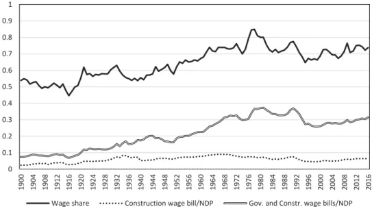
This article hypothesizes that employment in sectors relating to welfare policy has had a spill-over effect on the wage share in sectors without such a clear tie to active government policy. In line with measurement made by Pensiero (2017) the main independent variables according to this hypothesis are the wage bill (employment times wages) of the government and construction sectors, relative to the size of the economy. Justification for the inclusion of the wage bill of the construction sector is given by the specific historical context in the Swedish case, accounted for below.Figure 1compares these variables over time in Sweden during the period of investigation.
The comparison of the variables presented inFigure 1suggests a close long-run relationship between the private non-construction wage share and the sum of the wage bills of the government and construction sectors relative to NDP (Gov. and Constr. wage bill/NDP inFigure 1), separated by a constant. The most salient deviations seem to have occurred before World war One and during World War Two. The historical account in this section reveals how and why there has been such a long-run connection between these variables in the Swedish case.
The starting position of the distributional struggle between labor and capital at the beginning of the twentieth century was to the advantage of capital. This was the dawn of an entrepreneurial age, when new companies were formed around innovations based on electricity and chemistry. In the meantime, the living conditions for the growing working class were often harsh. Real wages grew, but real profits grew more. The mechanization and commercialization of agriculture and the industrial expansion in the cities spelled rapid urbanization at the end of the nineteenth Century, and the resulting housing shortage was a source of continuing political concern in the early twentieth Century, as was the monotonous and routine work in the factories, long working hours and lack of democracy. The foundation of the workers’ party Sveriges Socialdemokratiska Arbetareparti (SAP) in 1889, and the trade union confederation Landsorganisationen (LO) in 1898 meant that the working class was a force to be reckoned with. Liberals tried to defuse the social unrest, and thereby socialist sentiments, for instance via electoral reform and by addressing the housing shortage through favorable housing loans (Ramberg.,2000, p. 16). After the general political strike for universal suffrage in 1902, the employers formed Sveriges Arbetsgivareförening (SAF) in order to coordinate their efforts. A showdown came with ‘Storstrejken’ in 1909, a general strike and lockout involving about 300.000 workers. LO lost the battle, and the wage share continued to decrease, and its lowest point in the whole 1900–2016 period was reached in 1916.
Political tensions intensified again during World War One and with the Russian revolution in 1917. The revolutionary tide in Russia and in the rest of Europe meant that the socialist threat was more real than ever, and with the help of liberals in the parliament, the working class parties (which split into two in 1917) finally managed to push forth universal male suffrage in 1918. In 1919 the parliament voted for the introduction of the eight hours workday, and in 1921 the women con-quered suffrage as well. The wage share increased rapidly, partly because of worker militancy (Bohlin & Larsson,2007) and the implementation of the eight hours workday (Bengtsson,2014b), but also because of the deep depression of 1921–1922, which shrank profits faster than wages. The unions increased both in strength, measured as union density (Kjellberg,2017), and militancy, measured as strike intensity (Edvinsson,2016b), throughout the 1920s. During the 1920s' crisis, the government established an employer of last resort program for infrastructure construction, but with wages much below those of the regular labor market.
0 0.1 0.2 0.3 0.4 0.5 0.6 0.7 0.8 0.9 1 1900 1904 1908 1912 1916 1920 1924 1928 1932 1936 1940 1944 1948 1952 1956 1960 1964 1968 1972 1976 1980 1984 1988 1992 1996 2000 2004 2008 2012 2016
Wage share Construction wage bill/NDP Gov. and Constr. wage bills/NDP
Figure 1.The wage share in private non-construction and wage bills of government and construction sectors, relative to NDP, in 1900–2016.
As SAP gained strength, it formulated bold visions about‘Folkhemmet’ a progressive welfare state for the Swedish people. The revolutionary fervor and Marxist rhetoric were gradually exchanged for a more pragmatic and even nationalist stance (Sejerstad.,2011, pp. 159–162). When SAP gained the government power in 1932 it started to put words into action. The global Great depression and the associated political turmoil that followed propelled new ideas about economic policy, and Swedish social democracy was quick to pick them up. In 1933, SAP introduced‘beredskapsarbeten’, with jobs in the state and the municipalities– this time with wages and conditions more similar to those in the regular labor market. According to Lewin (1967, pp. 59–80), the long-term goal was to resist wage cuts and to strengthen the position of labor over capital. The growth rate of the ratio of public investments doubled in the 1930s compared to the 1920s (Edvinsson,2005), and the government stimulated house construction through low interest rates and allowances for the residents, both in order to tackle unemployment and to remedy the pressing housing shortage (Johansson & Karlberg,
1979, pp. 18). Already since the 1870s, local authorities were obliged to plan cities in a more organized way, so that dwellings, infrastructure and community buildings functioned in harmony– though their ability to enforce such plans were often limited. In the late 1920s and early 1930s, city planning intensified and became increasingly politicized (Hall,1991, pp. 179–213). The great push in housing would however wait until after the Second World War. The trend in the private wage share was more or less stagnant between 1920 and 1940.
The policy for high employment was an important precondition when LO and SAF met in Saltsjöbaden, Stockholm, in 1938. The treaty formed was an important part of what was to become known as‘The Swedish model’ – a historical compromise between Swedish capitalists and workers in the political and the economic realms. The deal would form the basis for labor market negotiations until at least the mid-1970s (Wennemo,2014, pp. 229–238), and was a prerequisite for the extensive central labor bargaining during that period (Kjellberg,2017).
The massive intervention by the government came already with the outbreak of the war however. In Sweden, capital controls and other regulatory measures were coupled with deficit spending. The efforts went beyond just maintaining employment at pre-war levels. In fact, unemployment among union members dropped from 11 percent before the war, to only three percent in 1946 (Molinder,
2012). When the Swedish labor movement´s postwar program was put forth in 1944 the inspiration was not from socialist theory but rather from the wartime economy, which had demonstrated the power of economic policy (Sejerstad.,2011, pp 293–294). The public sector grew fast in relative size, and private investment also regained vigor during the war, especially that in house construction. Although the relative size of the public sector shrank after the war, the decline was not as great as the wartime increase. The wage share increased.
Fears of a post-war depression proved to be ungrounded. Sweden was unharmed by the war and was in a good position to take advantage of the increased demand on the European continent. Again, the international threat of socialism, this time embodied in the Marshall plan to defuse socialism in Europe, helped advance the political power of the working class movement in Sweden. Apart from a drop in 1951 the wage share had entered on a growing trend that would last for about 30 years. The capitalist world entered a‘Golden age of prosperity’ (e.g. Marglin & Schor,
1990) and the rise of the welfare state was one of its most prominent hallmarks. In Sweden, this development went further than in other capitalist countries (Fulya,2005).
A crucial ingredient in the ruling SAP strategy was the Rehn-Meidner labor market model. In a nutshell, the idea was that more equal wages would make it harder for low wagefirms with low productivity and easier for high wage, high productivityfirms, thus increasing a tendency for the latter to grow. Active labor market policy and new social security systems would make the transition as smooth as possible for workers. At the same time, more equal wages would increase wages for predominantly female jobs in the government sector. Full employment, enforced through govern-ment actions, was a prerequisite for the model. Also, high growth would be distributed through the government services and result in better living conditions for the working class as a whole.
In a modernistic leap, SAP thus realized the visionary ideas of social engineering that had emerged in previous decades. The party launched an ambitious welfare program where the munici-palities had a central role in providing facilities such as daycare centers, schools, retirement homes– and housing for the general public. While agriculture went through a period of radical rationalization and mechanization, urbanization was rapid, and demand for new housing in the cities was pressing. A number of new suburbs were developed straight from the drawing boards of the city planners (Hall,1991, pp. 213–228). This also drove the construction of multifunctional suburb centers, with community facilities as well as spaces for private shop owners.
From the 1950s and onward a range of new regulations were introduced in order to steer resources to prioritized areas such as infrastructure and housing in the form of bonds. Additionally, the new public pension system founded in 1960 became an important buyer of the issued bonds. Housing construction kept growing until the late 1960s. Perhaps the most decisive move was the launch of the plan‘Miljonprogrammet’, with a target of one million new homes from 1965 to 1974. Municipality housing companies and non-profit cooperatives received beneficial government loans, and accounted for between half and two-thirds of all newly built apartments from 1951 to 1975 (Johansson & Karlberg,1979, p. 64).
Until then, industry had compensated for much of the loss of labor demand in agriculture, but although the sector experienced a shortage of labor with resulting foreign recruitment, the number of working hours in industry stagnated in the 1950s and 1960s. Productivity and mechanization were strong also in the industrial sector. The largest job increase was instead, by far, that in the public services, where the share of the total working hours more than doubled in the 1950s and 1960s. Expansion of the welfare services thus grew hip-to-hip with house and infrastructure construction. The corresponding increase in the share of construction working hours was about a third, and private services grew to a lesser extent (Edvinsson,2005). The wage share increased even as the workforce grew rapidly with labor immigration and– even more so, the entrance of women on the labor market. In the 1970s, this growth model ran into problems. The sense of a Swedish consensus from previous decades had shattered already around 1970 (Sejerstad.,2011, pp 333–334), and the economic down-turn that followed after of the collapse of the Bretton Woods currency system and the oil crises opened up a breach in Keynesian theory and policy internationally. The close connection between Keynesian ideas and the concept of the welfare state meant that both were challenged by new (or recycled old) economic thinking, globally as well as in Sweden. The crisis of Keynesianism paved the way for a new growth regime based on neoliberalism, globalization, andfinancialization which lasted from about 1980 throughout the rest of the investigated period (e.g. Dumeníl & Levý,2011). From a trending increase since the First World War, the trajectory of the wage share reversed. The profitability of Swedish enterprise was alarmingly low in the late 1970s (Edvinsson, 2010) and the succeeding devaluations of the Krona in 1977, 1981 and 1982 must be regarded as emergency acts. Nevertheless, they managed to invigorate not just the export industry, but the private sector in general. Residential- and government infrastructure investment, as well as the construction sector wage bill, began to shrink from about 1970 relative to the overall economy, as did the construction sector wage bill ratio to NDP, and the share of the public service sector began to shrink from 1980. Much of the institutional laissez-faire reforms came later however. Thefinancial markets were mostly deregulated in the latter half of the 1980s, and the goal of full employment was abandoned in favor of price stability in the early 1990s (Jonung,2017). The Rehn-Meidner model was gradually weakened in the new environ-ment of wage competition among unions, new economic ideas and institutional changes (Erixon,2010). House construction increased rapidly after the credit deregulation, only to decline even more after the housing market crash and the currency crisis in the early 1990s. Automatic stabilizers in the social security system drove thefinances of the state into deep deficits, full employment policy was abandoned, and the crisis pushed open unemployment up from 1.7 percent in 1990 to 9 percent only three years later. Sweden entered the kind of mass unemployment that other OECD countries had entered in the preceding two decades, and both household and functional income inequality increased fast (Ahnland,2017). The wage share shrank to levels last seen during World War Two.
The public debt put a straight-jacket on government consumption, which never recovered. During the mass unemployment in 1994, SAP– the party that called forth the Keynesian revolution in Sweden– introduced an extremely restrictive fiscal policy, a policy which was kept more or less intact throughout the rest of the period. Neither public employment nor employment in general would return to the levels seen before the crisis. House construction suffered long-term losses too. As part of the efforts to ‘sanitize the state budget’ the subsidized government house loans were scrapped, and the interest rate subsidies were lowered (Boverket,2007). After the crisis, housing shortage persisted, and house prices grew rapidly. The conditions got more similar to that of thefirst decades of the twentieth century.
Meanwhile, globalization increased in strength. The importance of trade grew, with imports plus exports even outgrowing total GDP in 2007. But the small deficit in the trade balance of the late 1970s had transformed into a massive surplus that persisted from the mid-1990s. In this sense, it was Sweden that out-competed other nations on the global marketplace. The wage share increased slightly from its low-point in the mid-1990s, as did government employment and employment due to government investment and housing construction, until the end of the period.
All in all, measures taken either to sooth demands and curb social disorder among the Swedish working class or to deliberately strengthen it relative to capital owners, were important drivers of social change until at least 1980. Ideas taking hold among social democrats in the 1920s regarding counter-cyclical economic policy, empowering the working class and engaging in the construction of a welfare state– Folkhemmet, were gradually manifested in real policy, starting in the 1930s and picking up pace after World War Two. In the 1970s however, the policy met a renewed resistance, and in the 1980s the tide had changed again, this time in favor of capital.
Methodology
The research aim of the present study is to assess the long-run impact of government job creation in the welfare services and in construction of infrastructure and housing on the wage share in the rest of the Swedish economy. The hypothesis is that such job creation has increased the bargaining power of the Swedish working class in general during the 1900 to 2016 period, resulting in a higher non-construction wage share. The delimitation in time is set because it roughly coincides with the rise and demise of the Swedish welfare state, and because of the availability of data (on union density). The main methodology in this task is time-series econometrics, and the analysis will be both on short- and long-run changes.
The dependent variable of the study is the wage share. In order to eliminate automatic correlation between the dependent and main independent variables, both government wages and construction wages and profits have been excluded from the measure of the wage share, so that this only measure the non-construction private wage share. Since capital depreciation is not consumed it is generally regarded as a more reliable measure to exclude depreciation from the functional income distribution, and thus when measuring the wage share (e.g. Karabounis & Neiman,2014). Total factor incomes correspond to value added in the national accounts, and the transformation of variables into ratios to value added at basic prices enables comparison to the wage share. Since the wage share is measured as a ratio to net factor incomes, it is necessary to measure other ratios net of capital depreciation too. This includes the main independent variables, the construction- and government wage bills (measured as Construction wage costs/NDP and Government wage costs/NDP).
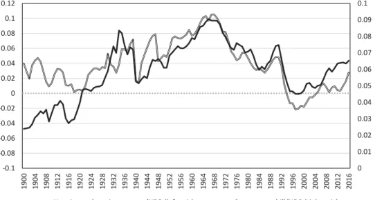
Figure 2depicts the wage bill of the construction sector relative to NDP and house and govern-ment investgovern-ment relative to NDP (negative values are due to capital depreciation being larger than new construction). Government investment includes the net investment in infrastructure such as roads and railroads, and of official buildings such as schools, hospitals, and military facilities, etcetera (Publicly owned companies are not included in neither government consumption nor investment). Likewise, housing investment is measured as the netfixed investment in residential services divided by NDP. Housing policy has very much been a part of the Swedish welfare policy. Allocation of
resources has been carried out both by the market and the state, and housing construction has been carried out by a mixture of private businesses, non-profit cooperatives and municipalities. In the post-World War Two era until the deregulations of the 1980s, the government controlled theflow of funds to the sector either directly through state loans or indirectly through extensive credit regula-tions. Policy has been guided by either labor market considerations and/or more direct social concern regarding living conditions of the general public. The building of dwellings and the construction of public welfare facilities and infrastructure, as well as space for private shop owners and the like, has been planned and executed in the same process by city planners with a political mandate. This suggests that construction work should be considered a compound variable, with a heavy influence of government policy during much of the period of investigation. Formal econo-metric testing validates this that house construction and public infrastructure investment are collinear throughout the period of investigation (not reported).
Even so,Figure 2, shows that the development of the wage bill of the whole construction sector relative to NDP is not identical to housing and infrastructure construction relative to NDP. This is because of two reasons. Firstly, the wage and profit shares of the construction sector have varied over time, and secondly, there is more construction in the economy than that of housing and publicly funded infrastructure– although the latter together form the bulk of all construction. The largest deviation between the two variables inFigure 1seems to have occurred before about 1920, when construction was less influenced by politics. A division of wages between construction of buildings for private enterprise and dwellings and buildings for welfare services and infrastructure is however not available due to lack of data.
Nevertheless, a reasonable conclusion while observing the available data is that the wage bill of the total construction sector ought to be a fairly accurate proxy for the wage bill in construction of housing and infrastructure, at least after 1920. The data on both the wage share and the wage bills are obtained from Edvinsson for 1900–2000 (Edvinsson,2005,2016a) and Statistics Sweden (2019), adjusted to the earlier series, from 2000–2016. NDP is measured at basic prices.
Trade openness is a proxy for globalization which is used widely in the literature, and is measured as imports plus exports relative to net domestic product. Capital intensity is a standard proxy for the use of machinery, and therefore automation, and is measured as the net capital stock of machines and
0 0.01 0.02 0.03 0.04 0.05 0.06 0.07 0.08 0.09 0.1 -0.1 -0.08 -0.06 -0.04 -0.02 0 0.02 0.04 0.06 0.08 0.1 0.12 1900 1904 1908 1912 1916 1920 1924 1928 1932 1936 1940 1944 1948 1952 1956 1960 1964 1968 1972 1976 1980 1984 1988 1992 1996 2000 2004 2008 2012 2016
Housing and gov investment/NDP (left axis) Constr wage bill/NDP (right axis)
Figure 2.Fixed investment in housing and government infrastructure, and the construction wage bill, relative to NDP, in 1900–2016.
equipment relative to net domestic product. Again, data for trade openness and capital intensity are from Edvinsson (2005,2016a)), and Statistics Sweden (2019). Union density, a standard proxy for union labor bargaining strength, consists of the share of union members of the employed workforce, with data from Kjellberg (2017). Moreover, all models include a stationary (and therefore long-run exogen-ous) variable– economic growth, as represented by the lagged change in NDP per capita (lagged because it is considered to be exogenous). Like before, the data on NDP are from Edvinsson (2005,
2016a)), and Statistics Sweden (2019), and data on population are from Statistics Sweden (2019). All of the mentioned variables need to be examined thoroughly before engaging in regression analysis. When comparing non-stationary variables in the long term, the primary interest is in comparing the levels of the variables. Yet, simply running a regression with non-stationary variables will lead to biased and inconsistent estimators if the variables are not cointegrated– that is if they are not sharing a common trend.
When assessing the relationships between variables, information regarding coefficients is not sufficient. It is also useful to look at properties pertaining to the variables themselves, particularly regarding measures of dispersion. For instance, big changes with a small coefficient can have the same effect as small changes with a large coefficient.Table 1contains a description of the statistical properties of each variable.
In order to determine whether there are long-run effects distinct from short-run effects that occur from one year to another, a number of tests have to be performed. First, unit root tests may identify if the variables are stationary or non-stationary processes. In order to test the presence of unit roots, the conventional ADF-test is used, both with a constant only and with a constant and a trend. Lag length is decided by the BIC information criteria and the maximum lag is set to 12. Unit root tests are performed also on the first differenced variables, since short-run mechanics require stationary variables infirst differences.
If the variables are non-stationary, which visual inspection of the main variables in Figure 1
suggests, long-term correlation may be determined via cointegration tests. More so, it is possible to separate long-run effects (beta coefficients) from short-run effects (alpha, or speed of adjustment, coefficients, manifest in the error correction term). This study uses the Johansen test, since it enables for estimation in a Vector autoregression (VAR) setting where it is possible to establish predictive power via Granger causality. The VAR methodology is particularly suitable for studies of relationships between endogenous variables, such as in the present investigation. The lag lengths of the under-lying VAR models are determined with the help of the BIC, HQC and AIC information criteria (IC) with a maximum lag length of four (because of the annual nature of the data). The most parsimonious IC is chosen. LM tests for autocorrelation up to the h lag order used are conducted for all VAR models, where models with autocorrelation are dropped. Since the Johansen test is fairly robust to non-normality in the error terms (Cheung & Lai, 1993), the only source for concern regarding non-normality is the VEC models. Since the wage share and the sector wage bill variables are of prime interest here, tests for non-normality are conducted on the VAR system as a whole as well as on the underlying VAR equations of the wage share and the sector wage bills. Non-normality is checked with the Doornik-Hansen method.
The critical values of the trace statistics for Johansen test for cointegration with an exogenous stationary regressor are obtained from Harbo, Johansen, Nielsen, and Rahbek (1998). See also Rahbek and Mosconi (1998) for further discussion. The Pantula principle is used in the order of the cointegration tests, where the most restrictive model is testedfirst, but since there are no critical values available for models with an unrestricted trend, only models with either a restricted constant or a restricted trend are tested (if there are no significant results with neither a restricted constant nor a restricted trend, only the results with a restricted constant are reported). The ten percent significance level is used as a threshold due to the low power of cointegration tests in general.
Vector error correction (VEC) models are VAR models infirst differences with an error correction term, but since this study is focusing on long-term changes, complete VEC models are left out of the
study, and only speed of adjustment – short term – coefficients are reported. One of the major advantages of VAR (and VEC) models is that they are treating all variables as endogenous, and allows for interpretation of several avenues of causation. Long-run relationships are often associated with inertia and path dependence which are generated by mutual feedback loops between variables (Pierson,2004, pp., 19, 21). This suggests complex patterns of causation.
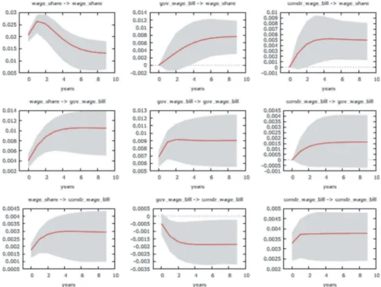
Finally, Impulse-Response Functions (IRFs) based on the VEC models are employed in order to visualize Granger causality. Such functions show how a shock of one standard error (standard deviation/root of the sample size) in an independent variable plays out over time for the dependent variable. The time-span used here is ten years. A boot-strapped ten percent confidence interval is applied to all IRFs, visualized as a grey area. IRFs are only reported for Models 1a and 2a, as reporting all IRFs for all models would result in too many graphs tofit in this article (but may be supplied on request). The results of all IRFs will however be discussed.
Two different setups of models are used, representing two ways of approaching the problem of measurement, but also a way of triangulating the results and achieve robustness. It is possible to interpret the wage bills of the government and construction sectors either as two separate and independent variables or as a combined variable measuring government job creation stemming from welfare policy in its totality. The benefit of separating them is that it enables an assessment of the significance of including the construction wage bill. If the latter is significant on its own, in justifies its inclusion. This is the approach used in Models 1a to 1d. However, the aim of this study is not to isolate or control for different aspects of government job creation through welfare policy, but to assess its overall effect. Thus, the sum of the wage bills of the government and construction sectors relative to NDP is used in Models 2a to 2d.
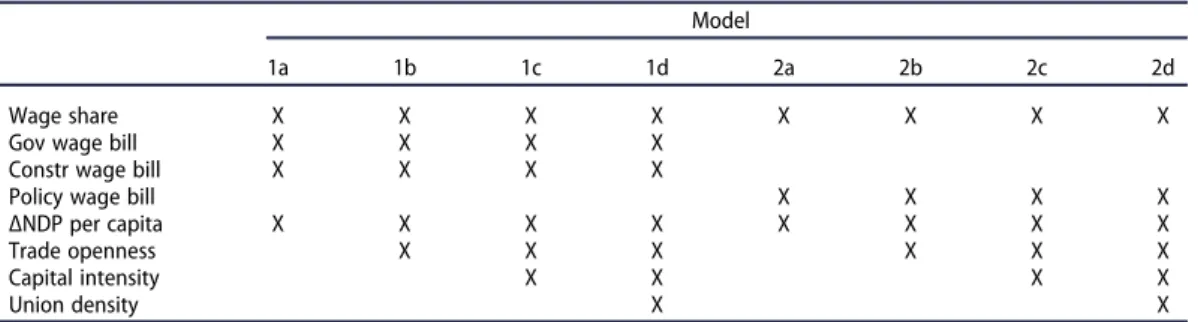
Thus, in Models 1a to 1d, the wage bills of the government and construction sectors relative to NDP appear individually, while in Models 2a they appear as a sum. Apart from the wage share, and the wage bills relative to NDP, Models 1a and 2a also include a lag of NDP per capita as an exogenous control variable (which is highly significant in the resulting VEC models). In unreported auxiliary models, each additional control variable then enters models corresponding to Models 1a and 2a one by one. In Models 1b to 1d and 2b to 2d, these control variables enter in a step-wise manner from the lowest t-statistic to the highest t-statistic (unreported Johansen tests also show that these models are cointegrated).Table 1provides an overview of the resulting models.
If no long-run relationships are detected in the Johansen test, further testing is stopped. Below, the long-run dynamics of the most extensive Models, Models 1d and 2d, are presented in algebraic form. In the equations and tables, the non-construction net wage share is referred to as the‘Wage share’, the ratio of the government sector wage bill to NDP is referred to as ‘Gov wage bill’, the ratio of the construction sector wage bill to NDP is referred to as ‘Constr wage bill’, and the combined wage bills relative to NDP is referred to as‘Policy wage bill’. Union membership density is referred to as‘Union density’, while capital intensity is referred to as ‘Capital intensity’, and trade openness is referred to as‘Trade openness’. The long-run equation of Model 1d can be written as:
Table 1.Model overview.
Model
1a 1b 1c 1d 2a 2b 2c 2d
Wage share X X X X X X X X
Gov wage bill X X X X
Constr wage bill X X X X
Policy wage bill X X X X
ΔNDP per capita X X X X X X X X
Trade openness X X X X X X
Capital intensity X X X X
Union density X X
Wage share ¼ β1 þ β2Gov wage bill þ β3Constr wage bill þ β4Trade openness
þ β5Capital intensity þ β6Union density þ u (1)
The long-run equation of Model 2d can be written as:
Wage share¼ β1 þ β2Policy wage bill þ β4Trade openness þ β5Capital intensity
þ β6Union density þ u (2)
In both the above equations,β is coefficient (β1 is constant), and u is the error term. In the other models (Models 1a– 1 c, and Models 2a – 2 c) variables and their coefficients are dropped according to the specification of the model.
Findings
In the following section, the properties of the variables and the results of the regressions arefirst presented in tables, to be discussed and analyzed in the text below.
Table 2summarizes key statistical properties of the variables. As the variables, except for NDP per capita and Trade openness, are stated as shares of a total, they span from zero to one. Unsurprisingly, variables with higher means and medians also have higher standard deviations. It is important to note that the coefficients from variables need to be interpreted in relation to standard deviations: Even though a coefficient may be large, the actual changes in that variable throughout the investigated period may not have been that large, so that the actual impact of one variable on another may still have been moderate.
Table 3contains the results from the unit root tests (ADF-tests with constant and with constant and trend) of the variables, which show that all are non-stationary in levels and stationary infirst differences at the five or one percent level significance level, except for NDP per capita growth which
Table 2.Descriptive statistics.
Mean Median Std. Dev.
Wage share 0.644 0.657 0.094
Gov wage bill 0.159 0.534 0.085 Constr wage bill 0.059 0.061 0.076 Policy wage bill 0.218 0.218 0.095 Union density 0.570 0.670 0.236 Capital intensity 0.412 0.494 0.171 Trade openness 0.689 0.575 0.277 ΔNDP per capita 2.381 2.815 4.431 Table 3.Unit root tests.
Constant Trend
Wage share −1.420 −2.514
ΔWage share −9.437*** −9.394***
Gov wage bill −0.985 −1.926
ΔGov wage bill −7.213*** −7.185*** Constr wage bill −2.339 −2.149 ΔConstr wage bill −8.113*** −8.154*** Policy wage bill −1.246 −1.853 ΔPolicy wage bill −7.176*** −7.166***
Trade openness −0.616 −2.472 ΔTrade openness −10.090*** −10.218*** Capital intensity −1.116 −1.240 ΔCapital intensity −8.638*** −8.635*** Union density −2.192 −0.650 ΔUnion density −6.593*** −7.025*** ΔNDPcap −5.830*** −5.818***
is stationary in levels (there is no need to test it in first differences). The results suggest that cointegration should be employed to test all variables in levels, and that NDP per capita should be added as an exogenous stationary variable in the error correction (EC) equations.
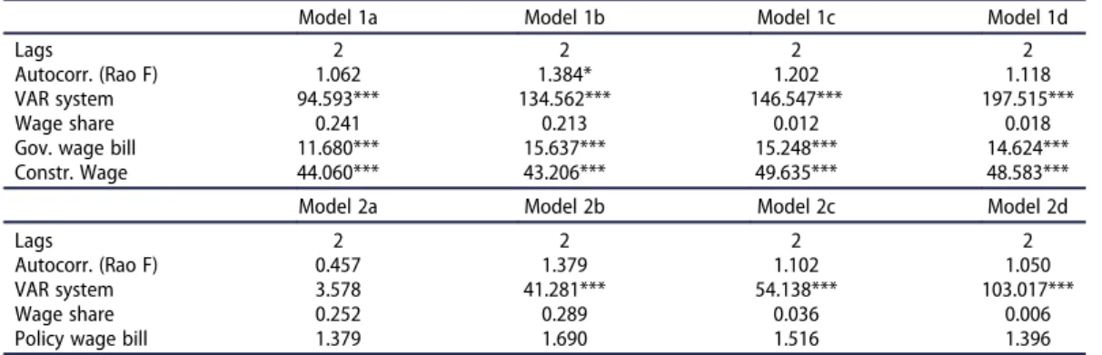
Depicted inTable 4, lag selection from the underlying VAR models with a maximum of four lags shows that either one or two lags should be included in all models, but further testing of models with those lag lengths reveal, as expected, significant autocorrelation in the models with only one lag. Model 1b shows signs of autocorrelation at the ten percent significance level, but this is considered acceptable. Hence, two lags are included in all models. Normality checks (the Doornik-Hansen test) detect non-normality in all VAR models except for in Model 2a, but a closer look at the equations for the individual dependent variables reveals that there is no non-normality in the Wage share equations. In Model 2a– 2d there is no non-normality in the Policy wage bill variable either.
Table 5 contains results from the Johansen tests for cointegration for all models. Since the cointegration tests for Models 1 c and 1d don´t indicate any long-run relationships, there is no further testing of the models (the focus in this study is on long-run relations). It must however be empathized that none of the control variables entered at this stage was found to be significant. When it comes to models 1a, 1b and 2a–2d, the Johansen cointegration tests show that there is one cointegrating relationship.
Further analysis of the long-term (beta) coefficients inTable 6display robust results for long-term correlation between the wage share on the one hand, and with the wage bill (as a ratio to NDP) of
Table 4.VAR diagnostics.
Model 1a Model 1b Model 1c Model 1d
Lags 2 2 2 2
Autocorr. (Rao F) 1.062 1.384* 1.202 1.118
VAR system 94.593*** 134.562*** 146.547*** 197.515***
Wage share 0.241 0.213 0.012 0.018
Gov. wage bill 11.680*** 15.637*** 15.248*** 14.624*** Constr. Wage 44.060*** 43.206*** 49.635*** 48.583***
Model 2a Model 2b Model 2c Model 2d
Lags 2 2 2 2
Autocorr. (Rao F) 0.457 1.379 1.102 1.050
VAR system 3.578 41.281*** 54.138*** 103.017***
Wage share 0.252 0.289 0.036 0.006
Policy wage bill 1.379 1.690 1.516 1.396
* = 0.1 significance, *** = 0.01 significance.
Table 5.Cointegration tests.
Model
Rank 1a 1b 1 c 1d
Rc. 2 lags Rc. 2 lags Rc. 2 lags Rc. 2 lags
0 47.281** 61.577* 80.962 102.620 1 12.104 21.968 40.442 59.264 2 1.803 10.354 19.867 36.725 3 0.061 8.836 21.072 4 1.689 11.467 5 3.432 2a 2b 2c 2d
Rc. 2 lags Rc. 2 lags Rc. 2 lags Rc. 2 lags
0 32.882** 43.111** 64.862** 83.445*
1 2.413 6.483 26.254 42.133
2 0.101 8.478 22.398
3 0.298 8.402
4 1.643
Rc denotes Restricted constant.* = 0.1 significance, ** = 0.05 significance. Harbo et al. (1998) do not provide critical values for the 0.01 significance level; hence, the 0.05 is used instead.
both the construction sector and the wage bill of the government sector. The coefficients for the government wage bill range from−0, 867 to −1, 019, which translates to a change in the wage share between about 90 and 100 percent coming from a one unit change in the government wage bill (the sign is reverted for beta coefficients in the output derived from Johansen cointegration). The coefficients for the construction wage bill similarly range from −0, 864 to −1, 188 which means that a change in the construction wage bill corresponds to a change between 90 and 120 percent as big in the wage share. Since the construction wage bill has a fairly low standard deviation relative to that of the government wage bill, the real effects on the wage share coming from the construction wage bill have not been too big when compared to the changes coming from of government wage bill. Still, an impact of the same magnitude from each variable seems to be very similar on the wage share. For the corresponding setups with the combined wage bill variable, the‘Policy wage bill’ in Models 2a and 2b also yields a coefficient very similar to that of the ‘Gov wage bill’ and ‘Constr. Wage bill’ in Models 1a and 1b. However, when more variables enter the Models, the coefficients succes-sively shrink, to−0,585 in Model 2d. This is hardly surprising, as consideration of more explaining factors often decreases the explanatory power of one single factor, even if none of the alternative factors are significant.
No other long-run variable other than the wage bills as they are defined can explain the wage share in the models. The only variable with some sort of significant results is ‘Trade openness’, but only at the ten percent significance level, and only in Models 2b and 2d. The coefficient is positive, indicating that the wage share is positively correlated with this particular measure of globalization. The constant is, as expected from the visual inspection ofFigure 1, significant in all models.
The most apparentfinding regarding the short-run coefficients inTable 7is that the wage share has a significant adjustment to the long-run co-movement in all the models. The speed of adjust-ment ranges from−0.226 in Model 1a to −0.272 in Model 2 c. This means that depending on the model, the wage share on average reacts to deviations from the long-term relationship within a time frame of about 4,5 and 5,5 years. This is a robust indication that the independent variables of the
Table 6.Long-run coefficients.
Model 1a Model 1b Model 1 c Model 1d
Wage share 1.000 1.000 – –
(0.000) (0.000) – –
Gov wage bill −1.019*** −0.867*** – –
(0.068) (0.102) – –
Constr wage bill −0.864*** −1.186*** – –
(0.351) (0.391) – – Trade openness −0.040 – – (0.027) – – Capital intensity – – Union density – Constant −0.416*** −0.393*** – – (0.018) (0.024) – –
Model 2a Model 2b Model 2c Model 2d
Wage share 1.000 1.000 1.000 1.000
(0.000) (0.000) (0.000) (0.000)
Policy wage bill −0.967*** −0.876*** −0.719*** −0.585***
(0.055) (0.064) (0.174) (0.198) Trade openness −0.039* −0.289 −0.043* (0.022) (0.023) (0.025) Capital intensity −0.100 −0.184 (0.101) (0.119) Union density 0.003 (0.057) Constant −0.417*** −0.408*** −0.408*** −0.390*** (0.014) (0.015) (0.014) (0.016)
model are able to explain variation in the wage share to a certain extent. Models 2c and 2d indicate that capital intensity may also be reacting to the long-run relationship detected by the Johansen cointegration test, but with a slower pace of 6,5 to 8,5 years (corresponding to coefficients of −0.149 in model 2d and−0.121 in model 2d).
Table 7.Short-run, speed of adjustment coefficients.
Model 1a Model 1b Model 1c Model 1d
Wage share −0.226*** −0.255*** -
-(0.067) (0.067) -
-Gov wage bill 0.026 0.014 -
-(0.026) (0.026) -
-Constr wage bill 0.020 0.018 -
-(0.012) (0.012) -
-Trade openness 0.666*** -
-(0.204) -
-Capital intensity -
-Union density
-Model 2a Model 2b Model 2c Model 2d
Wage share −0.230*** −0.246*** −0.272*** −0.263***
(0.067) (0.063) (0.064) (0.058)
Policy wage bill 0.043 0.029 0.024 0.015
(0.030) (0.029) (0.030) (0.027) Trade openness 0.652*** 0.650*** 0.631*** (0.191) (0.197) (0.179) Capital intensity −0.149** −0.121* (0.067) (0.062) Union density 0.107** (0.050) Standard errors are in brackets. * = 0.1 significance, ** = 0.05 significance, *** = 0.01 significance.
When assessing the IRFs of Model 1a inFigure 3, it is clear that shocks in both the government-and construction wage bills relative to NDP has a significantly positive impact on the wage share, at least after two to four years. A one standard error shock in the government wage bill of about 0,008 leads to a maximum impact of about the equal size on the wage share, while a standard error shock in the construction wage bill of about 0,007 leads to a maximum impact of about 0,005 the wage share. In Model 1b, Trade openness does not yield an impact on the wage share that is significantly different from zero. The IRFs of Model 1a also imply endogeneity, so that a change in the wage share has a positive impact on the wage bills of both the government- and construction sectors, relative to NDP.
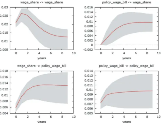
The IRFs from Model 2a inFigure 4are very similar to those of Model 1a, though being a bit larger and significant already after one year. A one standard error shock in the government wage bill of about 0,009 has a maximum impact of about equal that size afterfive or six years. This result is robust to inclusion of all control variables in Models 2b – 2d, though being of a somewhat smaller magnitude in the larger models but with significance already during the first year. Much like in Model 1a, Model 2a also yields a positive IRF running from the wage share to the combined‘Policy wage bill’, which again implies endogeneity.
Concluding discussion
The recent acknowledgment of the wage share as a crucial macroeconomic variable has shown that a number of variables either have a negative or positive impact. A central factor with a positive impact is the size of the public sector. In line with previous research on the international level, the present study indicates that in the case of Sweden in the 1900–2016 period, government creation of jobs in welfare services has been an important positive driver behind long-term changes in the
private wage share. The present study shows this notion to be valid also when government-induced job creation in the construction sector is included in the model. These two variables– the wages bill of public services and construction as ratios to NDP – need to be considered jointly in order to explain long-run changes in the Swedish wage share. A long-run relationship between the wage share and the wage bills of jobs induced by welfare policy, relative to the overall economy, is strongest when the wage bill variables are combined into one. This result hold when globalization, technology and union membership density are taken into account. This is a new and important finding. The results are however not as robust when the two wage bill variables appear as individual and independent variables (even though the control variables are not significant).
As is argued by Kalecki and others, these results suggest that generously paid jobs created via welfare policy have strengthened the bargaining position of workers versus private employers in Sweden. Earlier research shows that political leadership in Sweden was aware of such a connection in the formative 1930s and 1940s. From the 1930s onwards, Swedish governments provided unskilled and competitive jobs mainly in construction work, and in the post-World War Two period and until about 1970, they promoted well-payed jobs in both in the construction and government sectors when conducting social engineering in junction with the Rehn-Meidner labor market policy model. In the 1970s, it continued to expand public service jobs, while the construction sector started to shrink.
The government contributed to construction work directly through investment in welfare service buildings such as schools and hospitals, and roads and other infrastructure, as well indirectly through promotion of house construction via its housing policy– a particular aspect of the Swedish welfare policy. This was enforced through a range of measures, including city planning andfinancial regulation. Thereby, construction encouraged by government policy increased the relative size of the construction sector in general, and thereby the wage bill of the construction sector relative to the economy at large. More so, thefindings suggest that changes in the wage share have been caused by the wage bills of the government and construction sectors in the long-run. The adjustment of the wage share to deviations from the long-run relationship with the other variables is highly significant. Throughout the models, the long-run coefficients infer high correlation while short-run coefficients imply that the wage bills of the government- and construction sectors are drivers behind this co-movement. A unit change in the government wage bill or in the construction wage bill corresponds to approximately a change in the wage share of an equal magnitude, even though the speed of adjustment coefficient shows that it takes on average aboutfive years for the wage share to adjust. Likewise, IRFs show that a change in the government and construction wage bills to have significant and positive impacts on the wage share, and that this impact is gradual and occurs over several years. The results are particularly notable when the government wage bill and the construction wage bill are combined in one variable. There is evidence for mutual feedback as well: Though there are no negative and significant speed of adjustment coefficients for any of the wage bill variables, IRFs show that a shock in the wage share has had a positive impact on the wage bills, whether measured individually or combined. This suggests that a high and/or rising wage share may have created better conditions for SAP, the worker-led social democratic party of Sweden, to turn their political will into practice in the form of social engineering, represented by an expansion of welfare service jobs and jobs in the construction sector. A possible interpretation is that a high wage share may have been evidence for workers that SAP has been delivering in line with their interests, and this may have strengthened SAP in elections and increased their political power. This should come as no surprise: Mutual feedback loops are known to create the kind of long-run relationships investigated here.
When it comes to the negative and significant adjustment of capital intensity, it appears as if mechanization may be an outcome of increases in the wage share, although this cannot be corroborated by long-run coefficients. Trade openness does not seem to have been reacting to the long-run relationship significantly, though there is some evidence that it is positively correlated with the wage share in the long run. Models 2b and 2d show such a correlation at the ten percent significance level. Neither capital intensity nor trade openness has had a negative impact on the wage share, according to the results.
When it comes to union density, a measure of the bargaining strength of worker´s unions, there are no significant relationships detected either. In terms of Power Resource theory, this implies that the Swedish working class seems to have been more successful in increasing the wage share through political means rather than by labor market strategies. This corresponds to the notion raised by Blanchard (2006) and others, that effort for improving the conditions of workers is likely to be fruitless without an accompanying policy for full employment.
Even so, the results should be interpreted with caution, as it is possible that causal mechanisms may be operating at a higher frequency in time, for instance on a monthly basis rather than on an annual one. However, there are no such data available. Furthermore, the results accounted for above are obviously reliant on the quality of data in terms of reliability and validity, and other measures of for instance union strength, or any other variable in the study, may have rendered other results. Historical data on wage share determinants are hard to come by, and the data used are what is available.
The results of this study– that the creation of generously paid jobs by the government, both directly in public services, but also indirectly in the construction sector, has had a positive impact on the wage share– points toward the need for similar research on the wage share in other countries. Are thefindings regarding Sweden in this respect generalizable to other industrialized economies, or do they pertain to a specific Scandinavian or Swedish welfare model? Specific characteristics of the Swedish labor market institutions cannot be accounted for in a case study like this, but historical accounts tell us that these institutions are not simply given. For instance, the Rehn-Meidner model emerged at a point in time when the capital owners in Sweden had been significantly weakened, and the model succumbed when capital was on the rise relative to labor. Patterns of endogeneity have already been identified in the present study, but there may be more such interrelations to be discovered in future research. The present study may be seen as a starting point for quantitative assessment of the endogeneity inherent in Swedish class struggle.
History tells us that much of the advances in the wage share in Sweden in the twentieth Century at least partly can be seen as concessions to the working class during periods of social unrest and fear of socialism. Such was the case, at least partly, when a program for affordable housing was launched around 1900, when universal suffrage and the eight hour work day were implemented around 1920, and when the Marshall plan boosted European demand after World War Two. Labor governments or centrist or conservative governments with a ‘contagion from the left’ promoted full employment internationally. In Sweden, employment became a priority in the 1930s, and full employment was an important ingredient the Rehn-Meidner model. The strength of the Swedish working class can be seen both in the increases in the wage share and in the expansion of the welfare state, in line with the Power Resource approach of Esping-Andersen (1990) and Korpi (2002). The results of this study indicate that there was a mutual feedback loop between improvements in the wage share and the growth in scope and scale of welfare services. All in all, the success of the Swedish welfare state meant that the revisionist dream of taming capitalism for the benefit of the working class seemed to work for a long time in Sweden. The retrenchment of the Swedish welfare state from about 1980 was correspondingly associated with a decline in the wage share.
Disclosure statement
No potential conflict of interest was reported by the author.
Notes on contributor
Lars Ahnlandis affiliated with the Department of Economic History and International Relations at Stockholm University, Sweden, where he works as a researcher and senior lecturer. He holds a PhD in Economic History from Stockholm University, Sweden.
References
Ahnland, L. (2017). Inequality and bank debt in Sweden in 1919–2012. European Review of Economic History, 22(2), 1–24. Bengtsson, E. (2014a). Do unions redistribute income from capital to labour? Union density and wage share since 1960.
Industrial Relations Journal, 45(5), 389–408.
Bengtsson, E. (2014b). Labour’s share in twentieth–century Sweden: A reinterpretation. Scandinavian Economic History Review, 62(3), 290–314.
Blanchard, O. (2006). European unemployment: The evolution of facts and ideas. Economic Policy, 21(45), 5–59. Bohlin, J., & Larsson, S. (2007). The Swedish wage–rental ratio and its determinants, 1877–1926. Australian Economic
History Review, 47(1), 49–72.
Boverket. (2007). Bostadspolitiken: Svensk politik för boende, planering och byggande under 130 år. Retrieved fromhttp:// www.boverket.se/globalassets/publikationer/dokument/2007/bostadspolitiken.pdf
Caballero, R., & Hammour, M. (1998). Jobless growth: Appropriability, factor substitution, and unemployment. Carnegie-Rochester Conference Series on Public Policy, 48, 51–94.
Cheung, Y., & Lai, K. (1993). Finite-sample sizes of Johansen’s likelihood ratio tests for cointegration. Oxford Bulletin for Economics and Statistics, 55(3), 313–328.
Dumeníl, G., & Levý, D. (2011). The crisis of neoliberalism. Cambridge, MA: Harvard University Press.
Edvinsson, R. (2005). Growth, accumulation, crisis: With new macroeconomic data for Sweden 1800–2000 (Doctoral dissertation). Retrieved fromhttp://www.diva-portal.org/smash/record.jsf?pid=diva2%3A193148&dswid=−5537
Edvinsson, R. (2010). A tendency for the rate of profit to fall? From primitive to flexible accumulation in Sweden 1800–2005. Review of Radical Political Economics, 42(4), 465–484.
Edvinsson, R. (2016a). Data from: Historiska nationalräkenskaper för Sverige 1800–2000. Retrieved fromhttp://www. historia.se/
Edvinsson, R. (2016b). Data from: Stoppages of work (lockouts and strikes) in Sweden 1903–2005. Retrieved fromhttp:// www.historia.se/
Elsby, M., Hobijn, B., & Sahin, A. (2013). The decline of the U.S. labour share. Brookings Papers on Economic Activity, 2, 1–63. Englund, P. (1993). Del III: Bostadsfinansieringen och penningpolitiken. In L. Werin (Ed.), Från räntereglering till
inflationsnorm: Det finansiella systemet och Riksbankens politik 1945–1990, (pp. 153–193). Stockholm: SNS.
Erixon, L. (2010). The Rehn-Meidner model in Sweden: Its rise, challenges and survival. Journal of Economic Issues., 44(3), 677–715.
Esping-Andersen, G. (1990). The three worlds of welfare capitalism. Cambridge: Polity Press.
Fichtenbaum, R. (2009). The impact of unions on labour’s share of income: A time-series analysis. Review of Political Economy, 21(4), 467–588.
Fulya, F. (2005). An introduction to the Swedish welfare state. Istanbul Trade University Journal of Social Sciences, 4(7), 261–274.
Gornick, J., & Jacobs, J. (1998). Gender, the welfare state, and public employment: A comparative study of seven industrialized countries. American Sociological Review, 63(5), 688–710.
Guschanski, A., & Onaran, Ö. (2018). Determinants of the wage share: A cross-country comparison using sectoral data CESifo Forum 19(2), 44–54.
Hall, T. (1991). Urban planning in Sweden. In Hall (Ed.), Planning and urban growth in the Nordic countries(pp. 167–246). London: E & FN Spon.
Harbo, I., Johansen, S., Nielsen, B., & Rahbek, A. (1998). Asymptotic inference on cointegrating rank in partial systems. Journal of Business & Economic Statistics, 16(4), 388–399.
Hutchinson, J., & Persyn, D. (2012). Globalisation, concentration and footloosefirms: In search of the main cause of the declining labour share. Review of World Economics, 148(1), 17–43.
International Labour Organization. (2012). Global wage report 2012/13: Wages and equitable growth. Geneva: Author. International Labour Organization & Organisation for Economic Co-operation and Development. (2015, February). The
labour share in G20 economies. Turkey: Report prepared for the G20 Employment Working Group Antalya. Johansson, R., & Karlberg, B. (1979). Bostadspolitiken. Stockholm: Liber Förlag.
Jonung, L. (2017). Jakten på den stabila stabiliseringspolitiken. Ekonomisk Debatt, 45(4), 26–40. Kalecki, M. (1943). Political aspects of full employment. Political Quarterly, 14(4), 322–330.
Karabounis, L., & Neiman, B. (2014). Capital depreciation and labour shares around the world: Measurement and implications (NBER Working Paper No. 20606). National Bureau of Economic Research.
Keynes, J. M. (1963). Economic possibilities for our grandchildren. In J. M. Keynes (Ed.), Essays in persuasion (pp. 358–373). New York: W. W. Norton & Co.
Kjellberg, A. (2017). Kollektivavtalens täckningsgrad samt organisationsgraden hos arbetsgivarförbund och fackförbund (Studies in Social Policy, Industrial Relations, Working Life and Mobility: Research Reports No. 1). Lund: Department of Sociology, Lund University.
Korpi, W. (2002). The great trough in unemployment: A long-term view of unemployment, inflation, strikes, and the profit/wage ratio. Politics & Society, 30(3), 365–426.
Kristal, T. (2010). Good times, bad times: Postwar labour’s share of national income in capitalist democracies. American Sociological Review, 75(5), 729–763.
Lewin, L. (1967). Planhushållningsdebatten. Stockholm: Almqvist & Wiksell.
Lucifora, C., & Meurs, D. (2006). The public sector pay gap in France, Great Britain and Italy. Review of Income and Wealth, 52(1), 43–59.
Marglin, S., & Schor, J. (1990). The golden age of capitalism: Reinterpreting the postwar experience. Oxford: Clarendon Press. Marx, K. (1867/1990). Capital volume 1. London: Penguin Books.
McCallum, J. (1985). Wage gaps, factor shares and real wages. The Scandinavian Journal of Economics, 87(2), 436–459. Molinder, J. (2012). The determinants of unemployment in economic historical perspective– An analysis of wage setting,
total factor productivity and the warranted wage for the Period 1911–1960 (Bachelor thesis). Retrieved fromhttp:// www.diva-portal.org/smash/record.jsf?pid=diva2%3A547639&dswid=−4782
Organisation for Economic Co-operation and Development. (2012). Labour losing to capital: What explains the declining labour share? OECD Employment Outlook 2012. Paris: OECD Publishing.
Pensiero, N. (2017). In-house or outsourced public services? A social and economic analysis of the impact of spending policy on the private wage share in OECD countries. International Journal of Comparative Sociology, 58(4), 333–351. Pierson, P. (2004). Politics in time: History, institutions, and social analysis. Princeton: Princeton University Press. Pikettty, T. (2014). Capital in the twenty-first century. Cambridge, MA: The Belknap Press of Harvard University Press. Rahbek, A., & Mosconi, R. (1998). The role of stationary regressors in the cointegration test (Working paper).
Copenhagen: Department of Theoretical Statistics, University of Copenhagen.
Ramberg., K. (2000). Allmännyttan: Välfärdsbygge 1850–2000. Stockholm: Byggförlaget in cooperation with Sveriges allmännyttiga bostadsföretag (SABO).
Sejerstad., F. (2011). The age of social democracy: Norway and Sweden in the twentieth century. Princeton: Princeton University Press.
Statistics Sweden (2019). Data from: Statistikdatabasen. Retrieved fromhttp://www.statistikdatabasen.scb.se/pxweb/sv/ssd/
Stockhammer, E. (2013). Why have wage shares fallen? An analysis of the determinants of functional income distribu-tion. In M. Lavoie & E. Stockhammer (Eds.), Wage-led growth: An equitable strategy for economic recovery (pp. 40–70). London: Palgrave Macmillan.
Stockhammer, E. (2017). Determinants of the wage share: A panel analysis of advanced and developing economies. British Journal of Industrial Relations, 55(1), 3–33.