Modeling and Simulation of an Electrostatic Precipitator Including a Comsol Multiphysics Guide for Modeling an ESP

(1)

School of Computer Science, Physics and Mathematics Växjö, Sweden.

Degree Project

Modeling and Simulation of an Electrostatic

Precipitator

Including a Comsol Multiphysics Guide for Modeling an ESP

Muhammad Ahmad and Jhanzeb 2011-02-10

Subject: Electrical Engineering Level: Second Level (Masters) Course Code: 5ED05E

(2)

ABSTRACT

Gaseous exhaust of different industries contains dust particles of different chemical precipitates that are harmful for the environment. Electrostatic Precipitators are very often used in industries to filter their gaseous exhaust and to prevent the atmosphere to being polluted. Electrostatic Precipitators are very efficient in their work. Electrostatic Precipitators use the force of the electric field to separate the dust particles from gaseous exhaust. Electrostatic Precipitators charge the dust particles and remove these particles by attracting these charged dust particles toward the collecting plates. The charging of dust particles requires a charging zone. When gas passes through that charging zone, the dust particles in the gas stream become charged and then these charged particles are attracted toward the collecting plates. The design of an Electrostatic Precipitators requires the knowledge of its working principle and the problems that often arise during its working. This thesis is the study of the working and the problems of the Electrostatic Precipitators. The main reason for problems in working of an Electrostatic Precipitator is the dust resistivity. This dust resistivity affects the collection performance of an Electrostatic Precipitator. This thesis also contains the simulation of an Electrostatic Precipitator. In the simulation part, the Electric Potential and the Electric Field of an ESP is modeled in an ideal condition, when no gas is flowing through the ESP. The industrial software Comsol Multiphysics is used for the simulation. A Comsol Multiphysics guide is given in appendix of this thesis report that provides information about using this software.

Keywords: Electrostatic Precipitator, Industrial Exhaust Controller, Industrial Pollution Preventer, Flue Gas Cleaner and Dust Trapper.

(3)

ACKNOWLEDGEMENT

We would like to express our sincere gratitude to Matz Lenells for being such a helping supervisor and arranging Comsol Multiphysics software for us. Without his advice and unique guidance, this thesis would never have become a reality.

We are thankful to Staffan Carius for providing literature and helping book on Electrostatic Precipitators.

We are thankful to Therese Sjöden for guiding us in using Comsol Multiphysics.

Finally, we wish to express our thanks to our parents, who have supported us in every step of life.

(4)

CHAPTER 1 INTRODUCTION

1 .1 Goal of the Thesis

The goal of this thesis work is to model the electric field of an Electrostatic Precipitator and study the working principle of an Electrostatic Precipitator. The studies of the problems that arise during the working of an Electrostatic precipitator are also the part of this thesis report. When an Electrostatic Precipitator runs, we may experience a number of problems causing the performance to be much lower than expected. These problems are apparent dust resistivity, re-entrainment and back corona. These problems are discussed in this thesis. The techniques to overcome some of these problems are studied in this thesis. The working of an Electrostatic Precipitators is discussed in chapter 2. The problems of Electrostatic precipitators are discussed in chapter 5. The modeling of the electric field of an Electrostatic Precipitator is the main part of this thesis report. Comsol Multiphysics software is used for the simulation work. By use of the software Comsol Mulitiphysics, an electric field is modeled between the wire and the plate of an Electrostatic Precipitator. The model of the electric field is greatly simplified by; 1) Assuming only pure non-streaming air between the wires and the plates, 2) assuming only a stationary case, i.e. all potentials do not depend on time. Based on this model, simulations have been done, see chapter 6. One goal of this thesis work is to show how to use the Comsol Multiphysics. A Comsol Multiphysics guide is given in appendix of this thesis work, which shows how the model of an ESP is made. This Comsol Multiphysics guide might be helpful for new users who want to make models in Comsol Multiphysics software.

1.2 What is an Electrostatic Precipitator?

An electrostatic precipitator ESP is a large, industrial emission-control unit. It is designed to trap and remove dust particles from the exhaust gas stream of an industrial process by using the force of an electric field.

We need Electrostatic Precipitator in order to reduce pollutants emitted into the atmosphere. Electrostatic precipitators are generally able to remove more than 99% of the particles in exhaust, without having to force the air through a filter.

Electrostatic Precipitators mostly find their place in the following industrial processes. 1. Power Generation Units mostly coal power plants

2. Cement 3. Chemical 4. Metals 5. Paper

In many industrial plants, particulate matter created in the industrial process is carried as dust in the hot exhaust gases. These dust-laden gases pass through an electrostatic

(6)

2

precipitator that collects most of the dust. Cleaned gas then passes out of the precipitator to the atmosphere. Precipitators typically collect 99.9% or more of the dust from the gas stream [1].

1.3 Advantages of an Electrostatic Precipitator

Electrostatic Precipitators are capable of handling large volumes of gas, at high temperatures if necessary, with a reasonably small pressure drop, and the removal of particles in the micrometer range.

From page 8-9 in [2], “electrostatic Precipitators

1. Can be sized for any efficiency.

2. Can be operated at temperature up to 8500C. 3. Can be operated at fully saturated gas. 4. Has a low pressure loss.

5. Proven long life.

6. Acceptable electrical operating cost.” 1.4 Types of Electrostatic Precipitators

According to page 7 in [3], we differentiate ESP with respect to application in two types. These are wet and dry. The wet type retrieves wet particles, including acid, oil, resin, and tar, from the exhaust gas. The dry type, on the other hand, is used to remove dry particles like dust and ash.

1.5 Electrostatic Precipitation Theory

From page 5 in [4], “An Electrostatic Precipitator is a particle control device that uses electrical forces to move the particles out of the flowing gas stream. The particles are given an electric charge by forcing them to pass through the corona, “a region in which gaseous ion flow”. The electric field that forces the charged particles to the walls comes from electrodes, maintained at high voltage in the center of the flow lane.”

Once these particles are collected on the plates, they must be removed from the plates without retaining them into the gas stream. This is usually accomplished by knocking them loose from the plates, allowing the collected layer of particles to slide down into a hopper from which they are evacuated.

(7)

3

CHAPTER 2 WORKING PRINCIPLE

2.1 Basic Working Principle

According to [1], the working Principle of an Electrostatic Precipitator is best understandable by understanding six activities mentioned below:

Ionization - Charging of particles.

Migration - Transporting the charged particles to the collecting surfaces. Collection - Precipitation of the charged particles onto the collecting surfaces. Charge Dissipation - Neutralizing the charged particles on the collecting surfaces. Particle Dislodging - Removing the particles from the collecting surface to the hopper. Particle Removal - Conveying the particles from the hopper to a disposal point.

2.2 Construction of an Electrostatic Precipitator

For performing the above activities and efficient separation of dust particles from the flue gas stream the ESP constitutes a special construction which is generally the same for all wire-plate ESP but its size and working capabilities depend on the type of flue gas, gas volume, size of solid particles and dust characteristics.

According to page 5 in [4], Wire Plate ESP are used in a wide range of industrial applications including coal fired boilers, cement kilns, paper mills, oil refinery catalytic cracking units, oxygen furnaces, electric arc furnaces and glass.

In a wire-plate ESP, gas flows between parallel plates of sheet metal and high-voltage electrodes. These electrodes are long wires weighted and hanging between the plates or are supported there by mast-like structures (rigid frames). Within each flow path, gas flow must pass each wire in sequence as flows through the unit.

The ESP allows many flow lanes to operate in parallel, and each lane can be quite tall. This is the reason that these types of precipitators are suitable for cleaning of large volume of gas. The need for rapping the plates to dislodge the collected material causes the plat to be divided into sections, often three or four in series with one another, which can be rapped independently. The power supplies are often sectionalized in the same way for increased reliability. Dust also deposits on the discharge electrode wires and must be periodically removed.

2.3 Working of an Electrostatic Precipitator

According to page 6 in [4], the working of Electrostatic Precipitator requires a high value of DC voltage range that is supplied to electrode wire. The power supplies for the ESP convert the industrial ac voltage (220 to 480 V) to dc voltage in the range of 20,000 to 100,000 V according to the requirement. The supply system contains a step-up

(8)

4

transformer, high-voltage rectifiers, and sometime filter capacitors. The ESP may supply either half-wave or full-wave rectified dc voltage. There are auxiliary components and control to allow the voltage to be adjusted to the highest level possible without excessive sparking and to protect the supply and electrodes in the event of heavy arc or short-circuit occurs.

The voltage applied to the electrodes causes the air between the electrodes to become ionize. This ionization causes a corona discharge. A corona discharge is an electrical discharge that occurs when the air around a conductor ionizes. The strength of the electrical field must be great enough to cause the ionization. The electrodes usually are given a negative polarity because a negative corona supports a higher voltage than a positive corona before sparking occurs. The ions generated in the corona follow electric field lines from the wires to the collecting plates. Therefore, each wire establishes a charging zone through which the particles must pass.

At any applied voltage, an electric field exists in the interelectrode space. For applied voltage less than a value called “Corona starting voltage", a purely electrostatic field is present. When the value of applied voltage becomes higher than the corona starting voltage, gas near the electrode ionizes. This ionization, called corona, appears in the air as a highly active region of glow.

To initiate the corona discharge, the availability of free electrons in the gas region of intense electric field is required around the wire electrode. In case of negative discharge wire, these free electrons gain energy from the field to produce positive ions and other electrons by collision. The new electrons are in turn accelerated and produce further ionization, thus giving rise to a cumulative process termed as an electron avalanche. When the ionized particles pass each successive wire, they are driven closer and closer to the collecting walls. The turbulence in the gas, however, tends to keep them uniformly mixed with the gas. The collection process is therefore, a competition between the electrical and dispersive forces. Finally, the particles approach close enough to the walls so that the turbulence drops to low levels, and the particles are collected. Figure 2-1 shows the working of an ESP.

(9)

5

CHAPTER 3 THEORETICAL SIMULATION

The ESP operation contains many scientific processes. To best understand the theory of ESP, these scientific processes are described below. The principal action of an ESP is the charging of dust particles and forcing these particles to the collecting plate.

The following subsections will explain the different process theoretically. Electrical Operating Points.

Particle Charging.

Migration Velocity of Charged Particles. Collection Efficiency.

3.1 Electrical Operating Points

According to [6], the electrical operating points for an ESP are Voltage and Current. The value of corona depends on these electrical operating points. Therefore, the whole process of an ESP is mainly depends on the applied voltage and current.

The relation for corona discharge for an ESP is

I = AV ( V- Vc), (1)

where

A is a constant

Vc is the corona starting voltage

I is the electric current and V is the applied voltage.

At an electrode separation d > 5×10-2 m, the starting voltage of negative corona is 15d kV where d is the separation between the electrodes in cm.

As demonstrated at page 13 in [4], the electric field for producing this corona is determined experimentally. The electric field relation is

where

Ec is the corona onset field at the wire surface (V/m)

dr is the relative gas density and

(10)

6

According to page 14 in [4], Ec is the field that is required to produce corona. The voltage

that must be applied to wire to obtain this corona field, Vc is determined by this relation

where

Vc is the corona onset voltage (V)

d is the wire plate separation in meter (m).

According to page 14 in [4], No current will flow until voltage reaches this value. As voltage reaches this value, the amount of current flow speeds up and increases steeply above this value. The maximum current density on the plate directly under the wire is

where

J is maximum current density (A/m2) µ is the ion mobility (m2/Vs)

V is applied voltage and

L is shortest distance from wire to collecting plate.

According to page 15 in [4], the electric field between the plate and the wire increases with increases in applied voltage. A point will come when the electric field becomes a much stronger and further increase of voltage will not be possible without a spark. The value of the field when sparking going to start is given by this relation.

where

Es is sparking field strength (V/m)

T is absolute temperature (K) and P is the gas pressure (atm).

3.2 Particle Charging

As demonstrated in [6], particle charging is an important process among overall process of an ESP. The ions produced by corona discharge are the main cause of particle

(11)

7

charging. The particles are charged by the attachment of ions produced by the corona discharge. These ions are transported by either electric field and/or thermal diffusion. The particle charging by the ions transfer by electric field is called field charging. Field charging is more dominant for larger particles ≥ 2 µm, and for smaller particles ≥ 0.2 µm, thermal diffusion charging is more dominant.

The charge of a spherical particle is given by

where

q∞ is saturation charge ( C )

t is the charging time (s )

τ is the time constant of the field charging (s) ε0 is the permittivity of vacuum 8.85×10-12 F/m

εs is the specific permittivity

dp is the particle diameter (m)

E is the field strength (V/m) and J is the current density (A/m2).

According to [6], the saturation charge q∞ is proportional to the electric field strength.

The time constant τ is inversely proportional to the ionic current density J. Therefore, in order to impart a high particle charging, E and J should be high.

(12)

8 where

is a charge constant ( C )

is the time constant of the diffusion charging ( s ) K the Boltzmann constant ≈ 1.38×10-23 j/K

T is the temperature ( K )

e is the electronic charge ≈ 1.6 × 10-19 C Ci is the thermal velocity of ion (m/s)

ni is the number density of ions in space (m-3)

mi is the ion mass (kg)

µi is the ion mobility ( Vm/s2)

E is the field strength (V/m) and J is the current density (A/m2).

3.3 Migration Velocity of Charged Particles

According to [6], the migration velocity is the velocity of the charged particles by which these particles travel toward the collecting plate. The Coulomb force of a suspended charged particle in an electric field is

F = qE (13) where

F is the Coulomb force (N) q is the positive charge (C ) and E is the electric force (V/m).

The force on the moving charge particle is given by

Where, ωe is the velocity of charged particles that move toward the plate.

(13)

9 where

ωe is the migration velocity (m/s)

µ is the viscosity (Pa s)

dp is the diameter of particle (m)

Cm is the Cunningham correction factor

is the mean free path of gas molecules (m) T is the temperature (K)

P is the pressure (Pa) and

= 0.07 micro meter for air at atmospheric pressure and room temperature (300 K). For field charging, the migration velocity is written as

The migration velocity is proportional to the particle diameter dp and to the square of the

field strength E2.

The migration in diffusion charging is

3.4 Collection Efficiency

According to [6], the collection efficiency of an ESP, η is given by,

where

ωe is the migration velocity (m/s)

(14)

10 A is the area of the collecting electrode (m2) and Q is the gas flow rate (m3/s).

Collection efficiency is affected by following factors Geometry of the electrode.

Characteristics of the dust particles.

Collection efficiency can also found by this relation

where

L is the length of the collecting electrode along the gas stream (m) vo is the gas velocity (m/s)

b is the separation between the discharge electrode and the collecting electrode (m) and K is a correction factor determined from actual measurements.

t0 is called detention time and the vo is the gas velocity. These are important factors for

determining the performance of an ESP. By substituting detention time relation in above efficiency relation, we get this relation

If we concern the effect of voltage and the current on the collection efficiency, the following relationship is obtained. This relation is useful in industrial ESP

In industrial application the value of n is used is 2. Higher collection performance of an ESP is achieved by operating in maximum available voltage.

(15)

11

CHAPTER 4 CAPACITANCE CALCULATION

Capacitance between a wire and infinite plate

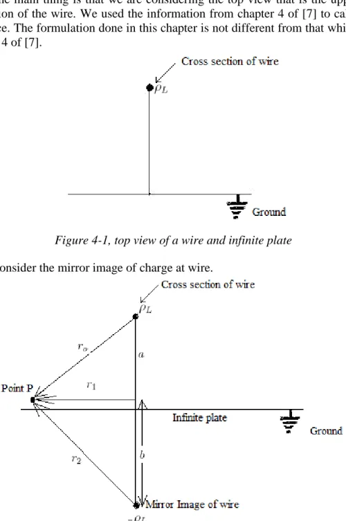
We have to find capacitance between a wire and an infinitely plate. We have an infinitely long plate which is connected with ground at one side. We have a long wire, and we have to find capacitance between infinitely long plates and the wire containing the line charge, but here the main thing is that we are considering the top view that is the upper part or cross section of the wire. We used the information from chapter 4 of [7] to calculate the capacitance. The formulation done in this chapter is not different from that which is done in chapter 4 of [7].

Figure 4-1, top view of a wire and infinite plate Now we consider the mirror image of charge at wire.

Figure 4-2, mirror image of a wire and infinite plate

(16)

12 Electric field due to line charge is given by

where

is charge per unit length C/m is the radius

Now the electric field due to positive line charge is

And due to negative line charge the electric field is

The potential due to electric field E1 is given by

The potential due to electric field E2 is given by

Now the difference between V1 and V2 is given by V= V2

-

V1

(17)

13 Simplifying all this, we get

Now

And This implies

Where k is any constant

Simplifying equation 39, we get

Equation 40 represents a family of circles around positive line charge and negative line charge. These circles are equipotential lines around these charges. Circles corresponding to positive line charge for which constant k < unity and circles corresponding to negative line charge for which k < unity. Figure 4-8, page 167, in [7] shows the equipotential lines together with the electric field lines.

Now considering the figure 4-3, given below We can rewrite the equation 37 as

(18)

14

Figure 4-3, point charge and its image

Figure 4-5b, page 163, in [7] resembles with our figure 4-3.

From the above figure 4-3, our case has two triangles, triangle OMP and triangle OPi M, where Pi is the inverse image or mirror image of original charge.

Now we can place the image of line charge at a place, so that the < OMP = < OPi M

And we have assumed,

And we have assumed this relation to be constant based upon the result of equation 1. This constant remains same because when changes r also changes itself accordingly and the constant ratio remains same. Moreover point pi is also called the inverse of point of p with respect to circle of radius a. So we can develop a relationship as

(19)

15

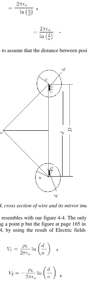
Now we draw the figure 4-4 to assume that the distance between positive and negative charges is D.

Figure 4-4, cross section of wire and its mirror image

Figure 4-6, page 165, in [7] resembles with our figure 4-4. The only difference is that, in figure 4-4 we are considering a point p but the figure at page 165 in [7], there is no point p. Now from the figure 4-4, by using the result of Electric fields E1 and E2, we can rewrite the potentials as,

And

(20)

16

From the figure 4-4, we have developed

From which we obtain

Using equation b in equation 52, we get

Since

(21)

17

CHAPTER 5 BARRIERS IN ESP PERFORMANCE

5.1 Apparent dust Resistivity

Apparent dust resistivity is the total resistivity due to the dust that is present between the wire and the plate of an ESP. Apparent dust resistivity depends on the resistance of the dust particles, and the temperature of the gas that flows through an ESP.

According to [6], the apparent dust resistivity ρd has major effects on the collection

performance of an ESP. Therefore, the knowledge of the effects of apparent dust resistivity on the working of an ESP is important. Dust particles form a layer on the collecting plates of an ESP. To reach to the ground-plates all ionic current must passes through this accumulated layer of particles. This layer of dust, with high resistance causes a reduction of field strength. The factors such as water content, gas temperature and the gas composition, effect ρd. Normally, the value of ρd at 150 to 200 oC lies within range of

102 and 5×108 Ωm. 5.2 Re-entrainment

From [6], “re-entrainment is the process of re-entry of collected dust particles into the interelectrode spacing. Some fine particles, however, also can re-entertain without collected on the plate. These fine particles are difficult to collect. In normal operation of an ESP, dust Re-entrainment takes place with rapping or carried over by increased gas velocity near the collecting electrode”.

When the apparent dust resistivity becomes < 1012 Ωm, and the adhesion of dust particles is poor, re-entrainment takes place. This badly affects the collection efficiency of an ESP. Conductive particles loose their charge when they are collected, and are charged to opposite polarity due to the induced charging. These particles are lifted into space by the electric field and then again, are charged by the corona discharge. These particles jump on the collecting electrode and go outside the ESP.

To eliminate the re-entrainment the following methods can be used. Adhesive agents can be used to cope with the re-entrainment of conductive dust particles. The adhesive agents, ammonia, ammonium sulfate or oil mists are used for this purpose.

Alternatively, rapping or scraping or brushing of collecting electrodes, is effective to prevent re-entrainment.

5.3 Back Corona

According to information from page 6 in [4], the layers of dust particles that accumulate on the electrode produce a hurdle in transportation of ionic current toward the collecting plate. When ionic current passes through this resistive layer to reach the electrode, this

(22)

18

ionic current produces an electric field in the dust layer. When this field becomes large enough it causes a local breakdown. When this occurs, new ions of wrong polarities are injected into the wire-plate gap where they reduce the charge on the particles and cause sparking. This breakdown condition is called "back corona". Wrong polarities ions are positive ions, and these positive ions tend to move toward the electrode that is creating a corona. On their way toward the corona wire, these positive ions collide with the negative ions that are moving toward the collecting plate, and hence reduce the overall field strength. This happens because when the positive ions collide with the negative ion these ions disappear and this thing causes the wastage of power. This phenomenon is termed as “Recombination of Ions”. The recombination is not favorable for the efficiency of an ESP and must be avoid to save power and to maintain the possible safe high value of electric field and current density to gain maximum precipitation.

From [6], “when the apparent dust resistivity becomes ρd ≥ 5×108 Ωm, back corona takes

place. Inside the dust layer on the collecting electrode, an electric field is established due to the corona current

Where

id is the corona current density (A/m2), and

Edb is the breakdown strength of the dust layer (V/m)”

When ρd increases, Ed becomes high, and an electric breakdown takes place when Ed

reaches Edb. From the breakdown point, ions of opposite polarity to the corona discharge

are emitted, resulting in neutralization of the corona. In case, negative corona is used, the breakdown causes positive ions propagating towards the discharge electrode. In the range of ρd between 5×108 and 109 Ωm, back corona causes excessive sparking. When going on an increase in ρd >1010 Ωm, the number of breakdown points in the dust layer

increases and finally the entire surface of the dust layer glows. A large number of opposite polarity ions are emitted into the space. This causes the reduction of the corona field. This back corona neutralizes the particle charging and the performance of ESP becomes down.

Various methods are used to treat with high resitivity dusts to reduce back corona.

Firstly, it can be controlled by varying the temperature and the humidity. When the temperature was lowered, the performance of the ESP increased sharply due to the elimination of back corona.

Intermittent energization is effective for abatement of back corona. The applied voltage is turned off before the surface charge accumulates to trigger a breakdown of the dust layer. During the voltage-off period, the surface potential decreases. This method is effective not only to improve the collection efficiency of high resistivity dusts, but also reduce energy consumption.

Pulse energization is also effective to reduce back corona. Instead of dc, pulsed voltage is applied. The ions emitted from the discharge electrode spread due to space charge, and a

(23)

19

more uniform corona current distribution can be obtained. For large scale ESP having large capacitance, durations of ms or µs can be used. To apply a pulse voltage, the ESP capacitance should be charged, and then discharged rapidly [6].

5.4 Corona Quenching by Space Charge

When the size of the dust particles is very small and their density is high then space charge is formed by charged particles. This reduces the field strength at the tip of discharge electrode, resulting in quenching of corona discharge. Sometimes the space charge enhances the field strength at the collecting electrode and causes flashover [6].

(24)

20

CHAPTER 6 SIMULATION OF AN ESP

The simulation of the Electrostatic Precipitator is the main part of this Thesis work. The software used for the simulation is Comsol Multiphysics version 4.1. Appendix A contains a guide to Comsol Multiphysics and how to model the stationary electric field in an ESP.

Our simulation involves the modeling of the Electric Potential and the Electric Field between the wire and plate of an ESP, when only pure non-streaming air is present between the wire and the plate. We are not simulating the whole process i.e., creation of corona region, charging of dust particles and migration of dust particles. Because, for simulating the whole process, especially the corona discharge, we must know about the behavior and nature of the gas. We are only simulating the electric field and electric potential when no gas with dust particles is flowing through the ESP. Simulation starts with drawing the structure of an ESP. Figure 6-1 shows the structure of an ESP. Height of the ESP is selected 1 meter. The distance between the wire and the plate is 0.25 meter. Wire to wire distance is 0.5 meter and the radius of wires is 2 mm. High level of negative dc voltage is applied at each wire and the plates are connected to the ground.

(25)

21

We divided the whole structure of the ESP into smaller parts called cells. One cell is shown in this figure 6-2.

Figure 6-2, one cell for simulation

The model contains many identical cells. We regard one cell for simulation because the results of the simulations of all the cells are identical. One cell is shown in figure 6-2. In Comsol Multiphysics, several steps are involved in making a model. These steps are explained in Appendix A. After making a structure, we have to define the material to our model. The material defined for wires and the plates are named as the conductor with conductor properties of Electrical Conductivity 1e6 S/m, Relative permittivity 1 and Relative permeability 1. We assumed air as a material between the wire and the plate. We selected Air with Electric Conductivity 1 S/m, Relative permittivity 1 and Relative permeability 1. In actual, the air has an electric conductivity of 8e-15 S/m at 20 0C. In an ESP, the value of electric conductivity depends on the condition of gas and the nature of the dust particles. The value of electric conductivity of air in an ESP no more remains the same as of the actual value of conductivity of air. The exact value of electric conductivity for a gas in an ESP is not yet measured. This is the reason that we used the value of air conductivity as 1 S/m.

(26)

22

We model the Electric Potential and Electric Field Intensity at different voltage levels, i.e. -30 KV, -50 KV and -70 KV between the wire and the plate of an ESP. We selected negative dc voltage. Electric Potential is applied at each wire of the ESP. These wires run along the height of an ESP as shown in figure 6-1. When a high voltage is applied, the air around the wire becomes ionized and current starts flowing through the air toward the grounded plate due to electron avalanche. We showed the distribution of potential from wire to the plate at different applied voltages.

Figures 6-3 to 6-5 show the electric potential distribution between the wire and plate.

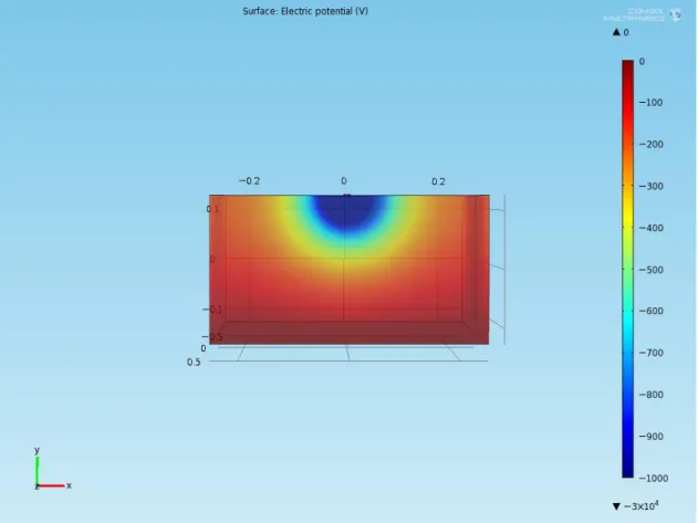
Figure 6-3, Potential distributions from wire to plate at -30 kV

Figure 6-3 shows the potential distribution from the wire to the plate at -30 kV. As it is clear from figure that potential distributes in such a way that it has high value at the wire and zero value at the ground plate. The vertical scale bar in the figure shows the value of different color. The dark yellow color has value of -400 V. According to color scale, there is high potential around the wire. This potential gradually becomes down and become zero, as shown by red color.

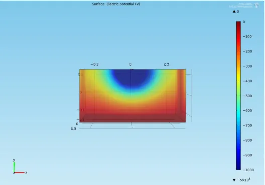
Figure 6-4 shows the potential distribution at -50kV. The color distribution is stretched in figure 6-4 as compared to figure 6-3. The dark yellow color moved away from wire, almost at the center of wire-plate spacing. The blue color area around the wire is increased, pushing the yellow color away from wire.

(27)

23

Figure 6-4, Potential distributions from wire to plate at -50 kV

At applied voltage of -70 kV, the figure 6-5 shows that the potential distribution in wire-plate spacing increased enough. The light green color appears at the center of wire-wire-plate spacing. According to vertical scale bar, the light green color has value of -600V. When we compare the potential distribution at three different voltage levels, we found that by increasing the value of applied voltage at wire the potential distribution in the different regions of wire-plate spacing increases.

(28)

24

When a voltage is applied to the wire, field is developed in the wire-plate space. When the value of applied voltage reaches Vc, corona starting voltage, current starts flowing

from the wire to the plate because of the ionization of air between the wire and the plate. The strength of this field is related directly to the applied voltage, as the Electric Field is the negative gradient of the Electric Potential. By increasing the applied voltage the filed strength increases. We examine the Electric Field intensity for different values of applied voltage. Electric Field intensity is more intense near the wire and becomes weaker gradually away from the wire toward the ground plate. The different color patterns show the strength of the field between the wire and the plate of an ESP.

Figures 6-6 to 6-8 show the electric field intensity between the wire and the plate of an ESP.

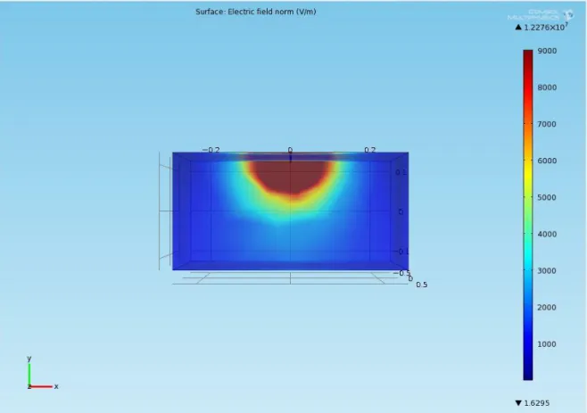
Figure 6-6, Electric Field V/m for -30 kV

Figure 6-6 shows the electric field intensity between the wire and the plate at -30 kV. The electric field intensity has high value near the wire as the red color surrounds the wire. The red color has maximum value, as shown in vertical scale bar. This red color gradually changes to yellow color showing that the electric field intensity decreased away from wire. The value of electric field becomes 6000 V/m at yellow region in figure 6-6. Similarly, yellow color changes to light green that has value of 4000 V/m. Finally this light green color turns to light blue and then becomes dark blue. Then the field becomes very much weaker at ground plate. At ground plate field value becomes only 1.6295 V/m.

(29)

25

Figure 6-7, Electric Field V/m for -50 kV

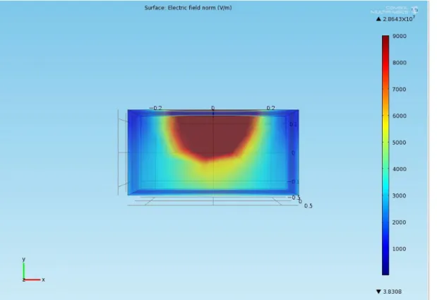
Figure 6-7 and figure 6-8 also show the electric field intensity at different regions in wire-plate spacing at different applied voltages.

(30)

26

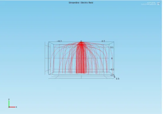
The figure 6-9 shows the distribution of electric field lines between the wire and the plate of an ESP. These lines emerges from the wire and end at the plate. In our simulation, distribution pattern of electric field lines remains same at three different applied voltage levels. The applied voltage only influences the electric field intensity (V/m) but not the electric field line distribution pattern between the wire and the plate. In figure 6.9, the electric field lines seem to cross each other. But in actual, the electric field lines do not cross each other. We have shown one side of 3D view in figures 6-3 to 6-9. If we cut the figure 6-9 in slices, the electric field lines view becomes clear and electric field lines no more seem to cross each other.

Figure 6-9, Electric Field Lines distribution pattern

Finally we are presenting the results of our simulation in table 6-1. This table shows the different values of potential and electric field intensity in wire-plate space at different voltage levels.

Potential ( V ) Electric Field Intensity ( V/m ) Voltage

applied

At the wire At the center of wire-plate spacing At the ground plate

At the wire At the center of wire-plate spacing At the ground plate -30kV -3×104 V -400 V 0 V 1.2276×107 V/m 5000 V/m 1.6295 V/m -50kV -5×104 V -600 V 0 V 2.0459×107 V/m 7000 V/m 2.7158 V/m -70kV -7×104 V -900 V 0 V 2.8643×107 V/m 9000 V/m 3.8308 V/m Table 6-1, Results of our Simulation

(31)

27

CHAPTER 7 CONCLUSIONS AND DISCUSSION

The most important things we have achieved are:

1. This thesis work describes how an ESP works, see chapter 2.

2. In chapter 3, we have collected basic formulas which can be used to model the different processes in an ESP.

3. The study of the problems that can arise during the working of an ESP, see chapter 5.

4. We have made a simulation of the stationary electrostatic field in an ESP, see chapter 6.

From different literatures and books, we studied about Electrostatic Precipitator that it performs outstanding cleaning of the gaseous exhaust of different industries, especially the coal power plants. The 99% collection efficiency makes Electrostatic precipitator the most desirable cleaning unit for different industries. Electrostatic precipitators have very high efficiencies due to the strong electrical forces applied to the small particles.

The simulation results are shown in table 6-1 at page 26. The simulation and modeling of an Electrostatic Precipitator was an important task of our thesis work. In simulation part, we modeled the Electric Field and the Electric Potential distribution from the wire to the plate of an Electrostatic Precipitator. We have not simulated the whole process of an ESP. We only simulated the electric field of an ESP when only air is present between the wires and the plates of an ESP. It could be the future work of this thesis to model the ESP in a loaded condition. Loaded condition means when some exhaust gas with dust particles is flowing through the ESP. We used Comsol Multiphysics software for making the simulation. The simulation was not an easy task. For making simulation in Comsol Multiphysics, the knowledge of this software was required. We worked on this software and got help from the online tutorials. We attended the Comsol Multiphysics workshop held in Växjö. Finally, we have been successful in making our model. We modeled the electric potential distribution and the electric field intensity that depends on the value of applied voltage. Higher the applied voltage, higher is the electric field intensity. Computations are done at -30 kV, -50 kV and -70 kV. We found that at applied potential, electric field distributes between the wire and the plate, as shown in chapter 6. The color distribution from the wire to the plate, in simulation, shows the intensity of electric field and electric potential in the region between the wire and the plate. Figures 6-3 to 6-8 show the electric potential and electric field distribution between the wire and the plate of an ESP. The streamlines in figure 6-9, show the pattern in which the electric field lines distribute from the wire to the plate.

According to the results presented in table 6-1, we analyze that when we apply high voltage at the wire, the electric field near the wire becomes very strong and starts decreasing in its value as move far from the wire towards the plate. Similar is in the case of electric potential. Electric potential is very high near to the wire, becomes low away

(32)

28

from the wire and becomes zero at the plate, as plate is connected to the ground. From the results, we also analyzed that if the wire-plate spacing in increased the electric field intensity becomes low. To maintain the same value of electric field intensity, the applied voltage must be increased. Hence electric field intensity is influenced by applied voltage. The electric field lines emerge from the wire and scattered on their way toward the plate. The electric field lines bend near the wire and then go straight toward the plate, as shown in figures 6-9 in chapter 6. As the electric field is a negative gradient of the potential, the color distribution is opposite in electric potential and electric field simulations. In Electric potential simulation, figures 6-3 to 6-5, blue color is present at wire and around the wire. This blue color gradually changes to yellow color and then changes to red color from the wire to the ground plate. Color distribution is opposite is case of the electric field, as shown in figures 6-6 to 6-8. This shows that the field is a negative gradient to the potential. We observed this distribution of potential and electric field intensity at different voltage levels.

In our model, we assumed that the Air has an electrical conductivity of 1 S/m, but its real value lies between 3e-15 S/m to 8e-15 S/m at 200C. We assumed 1 S/m because the real value of electrical conductivity of an ESP is not measured yet. The temperature during the working of an ESP becomes very high depending on the nature of exhaust. Different conditions of gas and nature of dust particles can change the electric conductivity of air from its real value to some new value. This is the reason that we have done our computations at a fix value of electric conductivity. The measuring of the exact value of air conductivity between the wire and the plate of an ESP can be the future work of this thesis. Modeling of an ESP based on the real value of electric conductivity can be a big success in the field of Electrostatic Precipitators designing in the future.

We studied some problems of the ESP from different knowledge sources. These problems are Apparent Dust Resistivity, Back Corona, Re-entrainment and Corona Quenching. The dust resistivity has major effect on the performance of an Electrostatic precipitator. Due to high dust resistivity, back corona and re-entrainment can occur. Due to re-entrainment, the dust particles that are collected on the plate lose their charge and go out into the air, hence reducing the performance. Back corona is produced due to recombination of ions. The recombination of wrong polarity ions with the right polarity ions causes the wastage of power. Pulsating dc voltage is favorable to reduce back corona. We used steady negative dc voltage in our model. The next version of this thesis work could be to model the ESP by using pulsating dc voltage or time varying voltage. By using the time varying voltage or pulsating dc voltage, the back corona effect can be avoided and power can be saved.

(33)

29 References

1. Electrostatic Precipitator Knowledgebase. Retrieved October 10, 2010, from http://www.neundorfer.com/knowledge_base

2. K. R. Parker, “Applied Electrostatic Precipitation” Blackle Academic & Professional, London, 1992.

3. Kjell Porle (ed.), Steve L. Francis, Keith M. Bradburn. “Electrostatic Precipitators for Industrial Applications” Rehva / Cost G3 June 2005.

4. James H turner, Phil A Lawless, Toshhaki Yamamoto, “Electrostatic Precipitator” Chapter 6, December 1995.

5. ESP Fundamentals. Hamon Research-Cottrell Pollution Control, Retrieved October 21, 2010, from http://www.hamon-researchcottrell.com/tech_espfundamentals

6. A Mizuno, “Electrostatic Precipitation”, IEEE Transactions on Dielectrics and Electrical Insulation, VOL 7, NO. 5, October 2000.

7. David K. Cheng “Field and Wave Electromagnetics”, 2nd Edition, Chapter 4. 8. Electrostatic Precipitator Theory and Design , Retrieved from October 27, 2010 ,

(34)

30

(35)

31

A Comsol Multiphysics Guide for Modeling an ESP

A.1 Introduction

In the today world, making computer simulations is an important part in the field of science and engineering. If we want to observe the real world physical laws in a virtual form then we have to take the help of computer simulations. And if we want to add a particular physics to our simulation, then we can do that by selecting from the available simulation making software. One of the options is Comsol Multiphysics software. Comsol Multiphysics also has several problem solving benefits, for example, when we start some project, this software is helpful in enabling to test various shapes geometries and their physical characteristics that are required in complex designs. We have made this tutorial by researching from already written material available in the form of books and tutorials, and here we will make our own general shape and try to explain it in a way to be understandable by any user.

Comsol Multiphysics allows the design to be optimized numerically before anything is actually fabricated. Making the model in Comsol Multiphysics requires the complete knowledge of physics that is involved in the model. In our model, physics of Electric and Magnetic field is involved. Comsol Multiphyics has an advantage that many types of physics are available in it. Physics of AC/DC, Heat laws, Structural Mechanics and Chemical reaction physics are present. One can choose any physics according to the requirement of the model. Making the models in Comsol Multiphysics is interesting in a way that we can apply different physics laws and parameters to the model graphically. We believe that it is a unique software in its use, and we think it is very user friendly. 3D models are easy to convert in a real world as compared to 2D models. If we want to analyze the 3D model in a real world it is easy to structure it as compare to make a real 2D model. In a real world, we can analyze our model as a building block. But in the technical sense a 2D model always solves quicker than 3D, and requires far fewer RAM. However, from analysis point of view it is better to use 3D option.

(36)

32

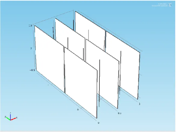
In figure A-0, an ESP model is shown. This model contains two wires and two plates. The wires and the plates are made of the conductor. The model is shown as a six side block. Air is the material inside the block. The two sides of the block are conductor plates, and the remaining four sides are insulated electrically.

As you create the model, each step is then recorded in the Model Builder. If, for instance, your model required a certain sequence of steps to get the right geometry, these would all be listed in the order you set. Even better, this series of steps can be edited and rerun without having to repeat the entire simulation [Ref .11, Page No. 9].

Now we will present a general example that was made by ourselves during the twenty five days experiments that we conducted on Comsol Multiphysics software by reading different online research manuals, by taking help from Mrs. Therese Sjöden and using online support from Comsol software website.

A.2 Two Wire Two Plate Model

In order to get acquainted with Comsol Multiphysics, it is best to work through a basic example step by step. The directions in this section will cover the essential components of the model building procedure, highlighting several features and demonstrating common simulation tasks along the way. At the end, we will have completed building a truly multiphysics model.

Now we will consider the case of our own created model. The model we are considering consists of two metallic rods that are connected in between two grounded plates. We are considering two metallic rods and two flat plates. We will apply voltage on the tips or cross-section of those two rods. And after applying ground effect on the two plates, we will join the rods in between the plates. Our goal is to simulate the electric field, the electric potential, electric field norm at different voltages.

The steps taken will be described as follows:

1. The first step is to open the Model Wizard, select a space dimension; the default is 3D. Click the Next button to continue to the Add Physics page.

(37)

33

Figure A-1, Select Space Dimension

2. Now add physics in the model. In the Add Physics widow, select “AC/DC”, in AC/DC list select “Magnetic and Electric fields” and then click on to go to next window.

Figure A-2, Add Physics Window

3. The last Model Wizard step is to select the Study Type. Select “Stationary Study” and then finish basic starting procedure by clicking the flag.

(38)

34

Figure A-3, Study Type Window

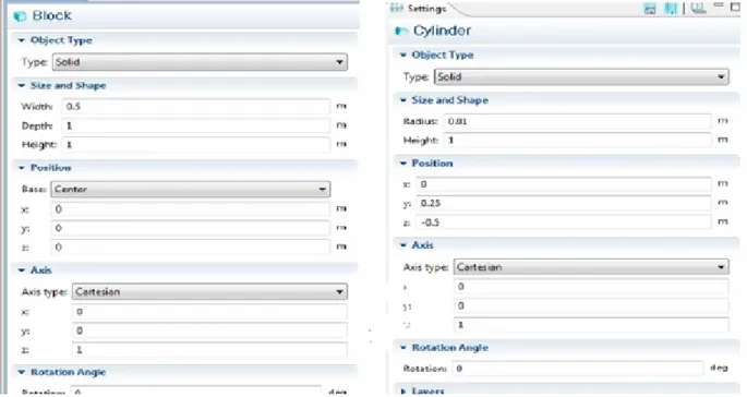
4. Now go into Model Builder window. In “Model 1 (mod 1)” select the “Geometry 1” option. There are several geometrical shapes available like sphere, block, cone and cylinder. Select from these geometrical shapes to build the geometry. In case, if the required geometry cannot be constructed then make geometry in Auto Cad software and import it to Comsol Multiphysics.

Figure A-4, Model Builder Window

Now from the “Geometry 1” option select two cylinders and two blocks. Adjust the lengths and radius of these cylinders to make electrode wires and adjust the blocks to make plane sheets. Click on these shapes and enter respective values for coordinates and lengths of these shapes in Settings window.

(39)

35

Figure A-5, Dimension and Geometry Size setting window

Now go to option “Global Definition” in Model Builder window. Right-click the “Global Definitions” and select “Parameters”. In the Settings window, enter respective values of parameters.

Figure A-6, Parameters Windows

(40)

36

Figure A-7, Required Geometry

Now go into the Model Builder window, click the “Form Union” node and then click the “Build All” button to run the geometry sequence.

Figure A-8, Form Union Window

5. Now add material properties to the geometry. For that, go to Model Builder window, right-click “Materials” and select Open “Material Browser”.

(41)

37

Figure A-9, Open Material

Now in Material Browser window, expand the Built-In materials folder, here a list of some materials opens, select the material from this list by right-clicking. Select “Air” from this list to add it as a material in between wire and plate.

Figure A-10, Model Builder extended

The material for wires and plates is “Conductor”. To add “Conductor”, right-click on “Materials” in Model Builder window, and select “Material”. Now add values for different parameters for this material in Material Contents window.

In the Settings window, locate the “Material Contents” section. The “Material Contents” section provides useful feedback on the model's material property usage. Properties that are both required by the physics and available from the material are marked with a green check mark. Properties required by the physics but missing in the material will result in an error and are therefore marked with a stop sign. A property that is not used in the model is unmarked. Enter the values of parameters as shown in following figure A-11.

(42)

38

Figure A-11, Material Content Window

In case of “Material Contents” of air, the electric conductivity, Sigma is not available which means its zero. Make the value of Sigma 1.

After selecting the material, apply this material to the geometry. For that, select the material then click on the specific part of geometry on which the material is to be applied. Right-click on the same part to confirm the material on a specific part.

Figure A-12, Conductor Rods

Apply the conductor property to the rods and side plates and apply air in the space between rods and two side plates.

(43)

39

Figure A-13, Conductor Plates

Now the figure A-14 will appear.

Figure A-14, Property Applied

For applying materials, select particular domains apply corresponding properties to these domains.

(44)

40

the model. The physics that is selected is “Magnetic and Electric field”. Now apply the properties like ground and potential to model. For that, in the Model Builder window, expand “Electric and Magnetic Fields” and examine its respective nodes to select the particular properties and apply them. Select “Magnetic Insulation”, which further contains three other properties. The purpose of selecting magnetic insulation is to protect the model from external magnetic and electric field interference. Apply “Ground 1” to two side plates and “Electric Insulation” to two rods.

Figure A-15, Model Builder Window

The electric insulation will be applied for all four boundaries of the model covering the two rods.

(45)

41

Figure A-16, Electrical Insulation

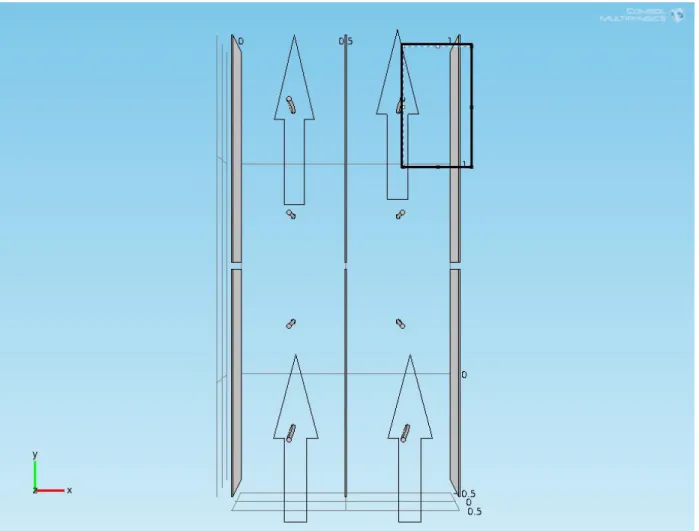
The “Terminal 1” mode is applied at the two rod tips, above tips and down tips of both rods as shown in figure. In “Terminal 1” mode enter the value of applied voltage. The output of the model will be shown according to the value of voltage entered at “Terminal 1”.

(46)

42

Apply initial values zero, so that later on changing these values give results at different values.

Figure A-18, Initial Value Window

7. Now the next step is meshing stage. A model can contain different mesh sequences for generating meshes with different settings. Mesh option is present in Model Builder window in “Model 1(mod1)” list. To add a mesh, do the follow following steps.

Right-click > mesh > right-click >free tetrahedral.

Figure A-19, Meshing

(47)

43

Figure A-20, Mesh Structure

By clicking on size option in the mesh the Size window will open. In “Element Size”, The size of Mesh can be changed.

Figure A-21, Mesh Setting Window

In this model, Mesh size used is “coarse”.

The coarse mesh size is used because by using the other meshing size the structure will not be visible.

(48)

44

8. The last step is to view the output of model. For that, go in the Model Builder window, right-click the Study node and go to study steps and then select “Stationary Study”.

Figure A-22, Compiling Model

The first output will be Electric Potential that we will get at applied voltage V = -30 kV.

Figure A-23, Electric Potential at -30 kV

After first output of Electric Potential at -30kV, change the value of applied voltage at the tips of rods by clicking on “Terminal 1” and enter the new value of voltage -50 kV. Repeat the same procedure of computing to watch the second output at -50 kV that is shown in next figure A-24.

(49)

45

By repeating the same procedure of changing value of applied voltage and computing the model the new output at -70 kV is shown in following figure A-25.

After observing the output for Electric Potential, now turn the output result from Electric Potential to Electric Field. For that, right-click on “Result” and then left-click the 3D “Plot Group”. Then expand the “3D Plot Group 1” and left click on “Surface 1”. A new window will open in settings tab. In expression bar click on the right most icon to open a drop list. That drop list contains different parameters for output. In these parameters select “Electric Field Norm”. The Electric Field intensity from wire to plate will show in output. By

(50)

right-46

clicking the “3D Plot Group” and selecting the “Stream Line” will show the Distribution of Electric Field in the form of lines from wires to plates by computing the model on different values of applied voltage. The following figure A-26 shows the procedure to change output parameter.

Figure A-26, changing the output parameter

The following figure A-27 shows the Electric field intensity and streamline at -30 kV

(51)

47

The following figure A-28 shows the Electric field intensity and streamline at -50 kV

Figure A-28, Electric Field at -50 kV

The following figure A-29 shows the Electric field intensity and streamline at -70 kV.