Regional Differences in
Returns to Education
An Analysis of the Italian Case from 1995 to 2014
MASTER OF SCIENCE IN ECONOMICS THESIS WITHIN: Economics
NUMBER OF CREDITS: 30 ECTS
PROGRAMME OF STUDY: Urban Regional and
International Economics
AUTHOR: Roxana Maria Lungu JÖNKÖPING May 2017
Master Thesis in Economics
Title: Regional Differences in Return to Education Authors: Roxana Maria Lungu
Supervisor: Lina Bjerke
Deputy Supervisor: Jonna Rickardsson Date: 2017-05-22
Human Capital, Education, Earnings, Regional Effect, Mincer Equation, Italy
Abstract
Return to education and regional differences have been amply studied in the literature, in particular by Human Capital and New Economic Geography studies. A combination of both these perspectives was not examined in the case of Italy regarding the North vs. South gap. The purpose of this thesis is to go one step further and to analyze regional differences in return to education across five macro-regions in Italy. The country’s unification is relatively recent, and this leads to expect that regional differences might be very high in magnitude. Mainly studies about Italy consider it merely from a North versus South perspective, identifying in the former the most advanced region both from an income and from an educational point of view. The regions in analysis are dividing the country into five areas that resemble its subdivision before the unification, hence the expectation to capture more insights about the difference respect to a North-South gap. The data are unbalanced panel data consisting of 8 variables, collected every second year for 20 years, for 7254 individuals, followed over time. The focus of this thesis is five regional analyses of the Mincer’s equation, one per each Italian macro-region. The results present significant differences in returns to education across regions, identifying the North-West and the South the leading ones, the North-East and the Center as in-betweens, and the Islands as lagging behind.
Table of Contents
1.
Introduction ... 1
2.
Background ... 3
3.
Literature Review ... 5
3.1 A Regional Perspective on Returns to Education ... 5
3.2 Ability bias and Signalling Theories ... 8
4.
Data and Variables Selection ... 11
4.1 Data ... 11
4.2 Regional Variation ... 12
4.3 Mincer’s equation ... 16
4.4 Dependent Variable ... 17
4.4.1 Income (versus Wage) ... 17
4.5 Independent Variables ... 17
4.5.1 Experience (versus Age) ... 17
4.5.2 Education and the “Sheepskin Effect” ... 18
4.6 Control Variables ... 19
4.7 Descriptive Statistics ... 20
5.
Methodology and Empirical Findings ... 22
5.1 Empirical Findings ... 23 5.1.1 Indipendent Variables ... 25 5.1.2 Control Variables ... 26
6.
Conclusion ... 28
7.
Limitations ... 29
8.
References ... 30
9.
Appendix ... 33
Figures
Figure 1: Data used in the estimation ... 15
Figure 2: Italian Reigns before the Unification vs. ISTAT macro-regions ... 33
Figure 3: Industrialization of Italy after the unification, and the North-South gap ... 34
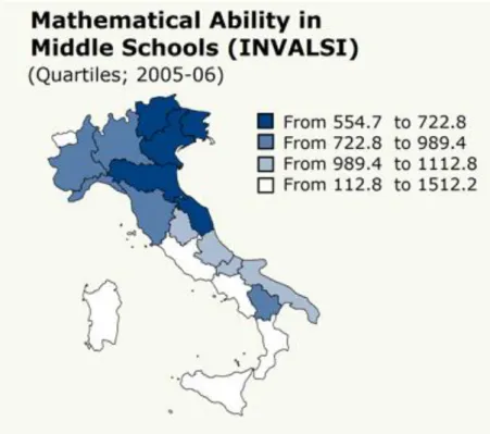
Figure 4: Mathematical Ability in Middle Schools 2006 ... 35
Figure 5: Annual Income per Capita (Euro), 2014 ... 35
Tables
Table 1 - Numerical Variables Description ... 21Table 2 - Dummy Variables Description ... 21
1. Introduction
Generally, the intra-country research on Italy focuses on the north versus south gap, as Italy is historically known to be a “Train moving at two speeds” as defined by Giovanni Giolitti, the Prime Minister between 1892 and 1921 (Lepre & Petraccone, 2012). Before unification, March the 17th 1861, Italy was fragmented in numerous autonomous reigns. Compared to
the other European countries the Italian unification occurred in very recent times, and as a consequence regional differences are still persisting. The previous reigns were brought together in an economic and political union, but the bringing together the population as a homogenous group turned out to be a much more complex task, that for certain aspects cannot be considered concluded even today. One could say that it was easier to create Italy, than the Italians. As an interesting proxy of cultural diversity, the UNESCO Atlas of the World’s Languages (2017) recognizes 32 different languages spoken in Italy. As a consequence of the regional diversity, the local power of the territory is still a debated subject as well. The regions are very powerful, and even if they do not account as a federation of states, they are all allowed a high degree of freedom in their self-regulation.1 As a historical
memory of the old reigns, the regions tend to present similarities within the old reigns’ borders. (Cavallaro, 2014).
Italy present difference in the income levels between the Northern and the Southern regions, as well as difference in educational results accordingly in the same areas: the situation seems to indicate that the Northern regions are richer and better educated, while the Southern ones are lagging behind.2 It might be possible to conclude that the income differentials might due
to different returns to education (Brunello, Comi, & Lucifora, 2000). A careful analysis considering difference among five macro-regions, going beyond the classical North-South view, can help in making light on the complexity of the country and its intrinsic heterogeneity and income differentials.
The purpose of this thesis is to analyze returns to education in Italy, accounting for the differences that occur at regional level, considering the division of the Italian territory in five
1 Some regions do have additional freedom through the so called “Special Statute”. The have legislative;
administrative and financial autonomy. They generally follow the general directives from the country, but are free to issue their own regulation in parallel, as long as not going against the constitution. They are the bilingual ones at the borders and the islands: Aosta Valley West), Friuli-Venezia and Trentino-Alto Adige (North-East), the island of Sicily and Sardinia.
macro-regions: North-West, North-East, Center, South and Island. These regions are defined by the Italian Institute of Statistics ISTAT (2017), and their extensions are nearly perfectly overlapping with the old reigns present on the territory before the Italian unification, except for smaller duchies consolidated together.3 The data is provided by the
Italian Institute of Statistics ISTAT, and consists of unbalanced panel data of 8 variables, collected every second year for 20 years, for 7254 individuals. Five regressions are estimated, each one for one Italian macro-region. A regression including the entire dataset is estimated as well, for comparison purposes. The regressions are an extension of Mincer’s (1974) equation, estimating as the independent variable the logarithm of income after taxes, and as dependent variables the level of education as the highest degree obtained, and the work experience as the number of years worked after studies. The square value of Experience, Gender, Work Branch, and Self-Employment are used as control variables.
The results confirm different returns to education across different macro-regions. In addition, every higher degree guarantees more than proportional returns than the previous one. The best performers are the North-West and the South macro-regions. Besides being the best one in general, they compare themselves showing respectively better returns in university level education and lower level education. At an intermediate level, we have the North-East macro-region and the Center macro-region, while the least important and less significant returns are in Islands macro-regions. An unexpected result came from the Work Experience, positive and significant in its linear term, it was not significant for any of the regression in its squared term, therefore not confirming the expected diminishing returns to human capital.
3 See Appendix for the “overlapping” details. A discussion of the macro-regions as well as a graphical
representation are presented in the “Regional Variation” section of the “Data and Variables Selection”part of this thesis.
2. Background
Brunello, Comi & Lucifora (2000) argued that in Italy the North is more industrialized, as the production is focused in the North, while more traditional and agricultural sectors are concentrated in the South.4 Industrialization is the result of a process of automatization,
digitalization, and higher mobility. The concept of industrialization is related to human capital, as more technical industries require skilled workers, and at the same time individuals with high human capital desire to locate close in proximity to industrialized and urban areas, in order to find better opportunities (Krugman, 1991). According to these arguments, income and education levels are expected to be higher in the Northern areas of Italy than in the Southern ones, which in facts it is the case, as showed claimed by Agasisti, Ieva & Paganoni (2017).5 It is not possible to state a priori if different income levels across regions
are determined purely by a regional factor, or because the returns to education in these regions are different. The theories behind Human Capital, in particular when regarded from a regional perspective, will help in answering this question.
Neave (1998) observed a link between quality of education and design of education policies. According to him, the schools are more and more interested in understanding the quality of education they are providing, in order to minimize the costs of education, while maximizing the results. As noticed by Neave (2012) Italy it is not an exception, and it is going through a process of redesign of its high education system, from a state-centric one to a university-independent one. Currently the education in Italy it is mandatory up the 16th year of age. The regular path is as follows: 5 years of primary education, 3 years of middle school, and 5 years of high school. The university studies are organized with the so-called “3+2” formula: 3 years of undergraduate studies + 2 of post-graduate. The 3+2 formula was introduced to adhere to European standards. In the so-called “Old system”, Italy used to have undergraduates of 4 years (MIUR - Ministry of Education University and Research, 2017). The rationale behind the reforms of the Italian education system was increasing the country’s competitiveness both at European and at national levels. For the academics, three important reforms happened in 1993, 1999 and 2010. The main reform of the public schools happened in 2000. Until the nineties, the main source of financing of the education system was the
4 Figures 2 and 3 in Appendix offer a graphical visualization of Unification and Industrialization processes in
Italy. The old Northern reigns are in correspondence with the currently most industrialized regions. 5 The graphical representation of can be found in Figures 4 and 5 in the Appendix.
central Government, as such, it had the power to issue directives regarding the scholastic decisions. Starting in 1993 the financing of universities was changed to a lump sum provided by the government to the academics but allowing them to allocate it freely. In 1999 control shifted almost entirely to the hands of the academics, including recruiting and subdivision of faculties and degrees. This introduced a quasi-market logic in the Italian education system, with the aim of increasing competition among national schools. The following year the same applied to all public schools. Lastly, since 2010, the universities are run de facto as corporations, with nearly zero intervention of the state. This, in turn, determined the importance of evaluative methods as signals of opportunities for improvements in education. In particular, the two main organisms dealing with evaluation are the “European Quality Assurance guidelines” (ENQA, 2017) for higher education, and the “National Institute for the Evaluation of the System of Education, Instruction and formation” (INVALSI, 2017) for lower education (Lumino, Gambardella, & Grimaldi, 2017; Vaira, 2011).
According to Docampo & Cram (2017), Italy is not very competitive in the international education system, as the time to graduation is above the European average. They also remark that Italy also has one of the lowest average incomes in Europe. Agasisti, Ieva & Paganoni (2017) argue that the North presents higher scores than the South on the national standardized tests, called INVALSI. In fact, by looking at the results of these tests the Northern regions perform better both in literacy ability and in mathematics, and this difference is persistent over time (INVALSI, 2017). In other words, where one is studying matters. Brunello, Comi & Lucifora (2000) identify big differences between North and South in income as well. Not only the Northern regions present higher returns, but they also show lower unemployment rate. At the same time, the Southern regions present the higher difference in return between state-employed and the employees of the private sector. The current study, differently from Brunello, Comi & Lucifora (2000), focuses on returns to education, rather than the education choice. From this perspective Brunello, Comi & Lucifora (2000) focus on the costs associated with education, while the current study with the benefits. Additionally, this study considers in more depth the regional perspective, as accounting not only for the North and the South, but for their subdivision into five regions: North-East, North-West, Centre, South and Islands. Lastly, the time period considered here goes from 1995 to 2014, while Brunello, Comi & Lucifora (2000) used the data from 1977 to 1993.
3. Literature Review
The literature that prepares the ground for the analysis mainly rests on literature on Human Capital theories, viewed from a regional perspective, as the Mincer’s equation will be used to for estimating the return to education. The New Economic theories allow to extend Mincer’s equation in order to account for macro-regional differences. Lastly the signaling theories are still an open and debated topic in the literature, which question the measurement of human capital by education, suggesting correlation between ability, education, and earnings.
3.1 A Regional Perspective on Returns to Education
Wage theories are a strictly related to Human Capital studies. Neoclassical economist initially proposed that a worker should be paid according to his contribution to production. With the marginal revolution, the concept of wage efficiency is introduced: workers are expected to be compensated by more than their marginal contribution, as a stimulus for increased productivity (Cowen & Tabarrok, 2011). Mincer (1974) formulates the relationship between Human Capital and earnings. The former is proxied by both years of education and work experience. They are both expected to have a positive effect on earnings. More recent literatures expand Mincer’s equation, in order to control for additional variables that can explain an increase in earnings, for instance intra-national disparities in the labor market, individual abilities or the level of education (Backman & Bjerke 2009, Cielslik & Rokicki 2016, Fally, Paillacar & Terra 2010, Hering & Poncer, 2010).
When faced with investment decisions, individuals apply cost-benefit analysis. The primary costs and benefits of education are those faced by the individual himself, however social and regional perspectives can apply as well. The student’s costs can be tangible, such as books and material, and intangible, intended as the opportunity cost of being out of the labor market. In other words, the choice of making an investment in education is taken considering expecting future returns. Therefore, the most obvious benefit from investing in education is the possibility of a substantial income increase. According to Wieseman (1965) the opportunity cost of education should also include forgone leisure as well, in addition to forgone income opportunities. At the same time, some “psychological” benefits could be considered too, for instance, the sense of enjoying the education process during the schooling period, and the knowledge coming from it for the rest of ones’ lifetime (Wiseman, 1965). The social benefits of education, according to Moretti (2003) are knowledge spillovers,
reduced negative spillovers (such as involving in criminal activities), and increased participation to the society’s welfare. In addition, according to Mincer (1974), since income is generally taxed proportionally, a high-income earner will give back to the society by paying “more” taxes. Both the psychological and the social costs and benefits of education are challenging and near impossible to asses, and as such will be a limitation to the current analysis. Regarding the regional perspective, Combes, Duranton, & Gobillon (2005) claim that the returns to education are determined in part by the economic environment of a region, as the benefits of education are gained in the local labor market. Therefore, is personal knowledge and ability can impact the returns to education, these cannot be expressed if not in a particular place, with its own characteristics, that will have an impact on earnings as well. The first formalization of the earnings-education relationship is attributable to Mincer (1974). He argues that the natural logarithm of earnings (in logarithm terms to ensure non-negativity) is composed of an additive function of education, and both the linear and quadratic value of experience (the latter is used as a control variable to account for diminishing return to experience), plus an error term.6 The original equation does not take into consideration
spatial perspective, therefore in order to account for it an extension of Mincer’s equation is necessary.
Assessing how much of the income is due to living in a particular region, and how much is due to a certain type of education is not an easy task. New Economic Geography theory is one groundwork that explains regional differences in income. Krugman (1991) uses NEG to explain the distribution of economic activities, as differentiated at regional levels. In particular, according to him there are two main regions: the core region and the periphery. The former is geographically large, high skilled, with intensive economic activity and high income; the latter is small, populated by low-skilled workers, relying heavily on the core region for economic activities, and with a low-income level. The concept that the size of a region affects the intensity of its economic activity is called the Home Market Effect. NEG does not necessarily have to be stand-alone theory. According to Head and Mayer (2006), regional income differentials can be explained through knowledge spill-over and human capital factors. The literature extending the Mincer’s equation with spatial
6 The equation and the theoretical aspects of the variables selection is discussed in details in the “Data and
characteristics such as the ones presented in NEG, in order to investigate regional returns to education, is subsistent, but it prevalently focuses on international regions (Martin & Rogers, 1995; Pflüger, 2004). Wang and Xu (2015) claim that the NEG model does not specify the size in choosing the regions, therefore, it is not required to restrain the research to big international analysis, but it is possible to focus within the same country as well. A step further in that direction is taken by (Backman & Bjerke, 2009) that focus on earnings differences across the regions in Sweden; by (Cieslik & Rokicki, 2016) on Poland’s regions; (Fally, Paillacar, & Terra, 2010) on Brazil’s regions and (Hering & Poncet, 2010) on China’s regions. These four papers are the very few that address workers’ heterogeneity in terms of individual earnings, as related to the regional disparities suggested by the classical NEG model. Their findings are that differences across regions in terms of return to education do exist within the same country.
Workers are not only a factor of production, and it would be an oversimplification to consider their location as a mere following of high-paying jobs. There is an extensive stream of literature discussing the role of amenities (such as good climate, clean air, natural elements and good infrastructures) in retaining skilled workers into a particular region, and the role of income and living costs (Rosen, 1979; Roback, 1980). The willingness to incur higher living costs in exchange for better amenities increases with income, or in other words, it is more likely to find skilled workers in locations rich in amenities (Ellickson, 1971). The intensity of economic activity is likely to result in pollution, the density of traffic etc. Even if from another point of view, the relationship between urbanization and high level of income is confirmed too: locations with a high level of negative amenities should offer workers higher earnings, in order to make them willing to stay (Roback, 1980).
Krugman (1991) identifies quality in skilled, rather than unskilled, workers. According to Hanushek and Dongwook (1992) the regional differences in returns are due to the “quality” of labor. According to Mincer (1974), to properly capture the positive impact of human capital on earnings, one should not only focus on education but on experience as well. In defining “human capital”, Glaeser (2005) sees it as going hand-in-hand with education. Florida (2012) has a similar view, but he suggests that education accounts only partially for human capital, while there should be something more, for instance, creativity or ability.
Hanushek and Dongwook (1992) claim that quality is a reflection of education, measured in years of schooling. Furthermore, Hanushek and Dongwook (1992) add that quality of labor
can be proxied by mathematical ability. Combes, Duranton and Gobillon (2005) are of the same view, and add that cognitive skills can play a role as well, and add that individual skills are explaining a great fraction of income differential. They claim that failing to account for them “will wrongly attribute earnings disparities to economic geography”. This risk can be overcome by working with individual data, instead of focusing on an aggregate level, in order to account for individual characteristics and experiences that can lead to higher returns. (Cieslik & Rokicki, 2016). In other words, NEG theories point out that there are regions (the core) more developed and with more intense economic activities than other regions (the periphery).
Human capital theories explain that workers with high human capital are more abundant in the former types of regions both because they are attracted by higher returns, and because they are most likely to be successful in these regions and to be selected by businesses demanding intensive exploitation of human capital and knowledge. (Behrens, Duranton, & Robert-Nicoud, 2013). Knowledge intensive sectors benefit from co-location and direct interaction; therefore, they are geographically bounded. In this view, the lower the distances among highly educated workers, the better the exploitation of their human capital is. As a result, knowledge intensive activities will tend to be concentrated within the same area (Feldman, 1994). Duranton and Puga (2004) claims that the concentration within a region is dictated by three agglomeration mechanisms: sharing, matching, and learning. Sharing refers to the sharing of all those inputs that can lead to economies of scale and specialisation. Matching refers to the matching between employees and jobs, as in a larger region in terms of economic activity the frictional unemployment can be eroded faster and with better results in terms of productivity, since there are more opportunities. Learning refers to the knowledge exchange and spillovers effects, that are more likely to happen as the interactions are more frequent, which is the case in the “core” regions.
3.2 Ability bias and Signalling Theories
Following Shaffer (1961), if human capital is proxied by education, and a certain level of education is mandatory by government requirements, it should not be considered as a private decision. However, according to Schultz (1961), compulsory education is in itself a signal of being the most valuable alternative: a government would only consider something in the best interest of the citizens to be set as mandatory. In other words, studies concerning returns to
different levels of education maintain their validity even under the circumstances of obligatory education.
Schultz (1961) opens up the discussion for education as signaling theory of other unexplained abilities, for instance creativity as assumed by (Florida, 2012). In this view, high return to education might be erroneously attributed to high education, while in facts they derive from higher ability. One solution could be the use of Instrumental Variables. In order to find a good instrument, it should be correlated with education, but not with ability, and as such it should also not influence income. According to Kaymar (2009) this could be represented by the year of birth, which is correlated with education as reflecting the schooling decisions made at a specific time. However, year of birth is also correlated with age, which is already present in Miner’s (1974) equation within the experience variable.
Measuring characteristics as ability by the use of an Instrumental Variable, it is a compelling task from an empirical point of view, as it can be a mix of intelligence, personality, attitude, etc. However, (Spence, 1973) claims that these abilities are already incorporated in the attainment of a degree, by the practice of signaling. An individual that has particular abilities knows that he has to communicate them to a potential employer. Therefore, the mean he has to signal that he is a high-quality worker is to attain a degree. In turn, an employer will value the obtaining of such credentials as correlated with higher ability and, therefore, with higher productivity. Firm, in facts, make hiring decisions based on expected productivity, and it is in the best interest of able employees to present all the available information regarding their abilities: therefore, an educational qualification is a signal that help in matching job opportunities and skilled employees. (Card, 1994; Deschenes, 2001)
According to Becker and Tomes (1986) the ability bias is overestimated, and its effect it is that small that it can be safely neglected, in particular according to Griliches (1977) only 1% of returns to education can be explained by ability. Additionally, Caplan (2006) claims that if signaling theory was accurate it will point out labor market imperfections. Namely, people would have an incentive to get degrees for the mere purpose of showing credential to future employers, and less able people will be pushed into the education system unwillingly to get an education, but just in order to get a signaling certificate. This, in turn, will not signal anymore ability and potentially higher productivity. Such situation would contrast with the logic behind the matching mechanism, which is instead one of the major agglomeration
forces behind Duranton and Puga’s (2004) explanation of difference in returns to education across regions.
4. Data and Variables Selection
In order to identify regional differences in return to education, the regional factor expressed by NEG is necessary, but not sufficient. There is more heterogeneity to be capture, and this can be done by accounting for HC. The main focus of this thesis is a regional analysis of the Mincer’s equation in the case of Italy. This section will discuss the choice of variables, the potential biases, and corrective mechanisms. The data in use is an unbalanced panel consisting of 7245 individual observations of 8 variables, collected every second year for 20 years
4.1 Data
The data in the analysis come from the so-called SHIW – Survey on Household Income and Wealth, compiled by the ISTAT – Italian Statistical Institute (2017) and available from the Bank of Italy (2017).7 This is a self-reported longitudinal study of the Italian population,
collected one every two years. The first survey to be used will be the one from 1995, so as to account for the introduction of the bachelor’s degree of 3 years, thanks to the 3+2 formula. The data collection did not follow a regular bi-annual path, going instead for three years, on two occasions: in 1998 and in 2016. The next wave is expected to be in summer 2017, after the completion of this analysis. Therefore, the data available come from the years: 1995, 1998, 2000, 2002, 2004, 2006, 2008, 2010, 2012, and 2014.
The data follows the individuals over time, they follow them for several years, and they take variables that consider their personal characteristics, therefore it is panel data. As coming from a longitudinal study, where people cannot be forced to consistently appear in the study (i.e. in case of death, or similar), it is unbalanced. Weights have been applied to account for such kind of bias.
The survey follows individuals over time, and it allows to follow a particular individual by attributing each one of them an identification number. The survey provides many data regarding individual characteristics, with identical questions over time. All the monetary amounts are expressed in Euros to make the comparisons easier, disregarding of the actual adoption of Euro in Italy. The base year for the deflator is 2010. The imputation methods
7 Details regarding the definition of all variables can be found on the Codebook of the dataset, we
of income and wealth are coherent across annual databases. The sampling design weights all the households in the sample by raking techniques “in order to align with the main marginal distribution derived from the socio-demographic statistics from ISTAT”. The rationale behind the sampling strategy is involves the use of unequal stratum sampling fractions in order to get unbiased estimates, even in the case of missing responses.
The data is used in a similar study performed by Brunello, Comi and Lucifora (2000). Their research is considering the biannual waves from 1977 to 1993, while the current study is taking the data starting from the most immediate next wave, in 1995 until the latest one in 2014, with the rational of accounting for the most recent reforms in the educational system. The regional variables considered by Brunello, Comi and Lucifora (2000) are the North and the South while the current study considers five macro-regions: North-East, North-West, Centre, South and Islands. Lastly, the main purpose of the current study is to analyze regional returns to education, or in other words the private benefits of education. Brunello, Comi and Lucifora (2000) dedicated a wider attention to the rationale behind the schooling choice. To mention is also the study of Lucifora and Meurs (2006), that uses partially the same data, but for a different purpose. Their research question is difference in gender pay gap between France, Great Britain and Italy. They also use the SHIW data but considering different variables, and in the specific they make distinction between male and female as employed in the private or public sector and as high skilled or low skilled.
4.2 Regional Variation
Agasisti, Ieva & Paganoni (2017) claim that the Italian education system is so fragmented that it appears to behave like three different markets: North, Center, and South. They suggest modeling this situation by applying dummies for the regions. As the North-South relationship in Italy is well established, it would be a good procedure to follow if dealing with only two or three macro-regions. The SHIW data offer more detailed insights, as they present a sub-division of the country in 5 macro-regions. In particular, these regions permit to analyses the differences that still persist after the unification of the reigns in the Italian state, as they are located in analogous territories.
For this reason, the current study will follow Agasisti, Ieva & Paganoni (2017) approach, starting with a baseline regression considering the regions as dummies. Then a second approach will use the macro-regions to divide the data in five and analyze them as if they were independent. It is the second one that will get the most meaningful insights on the Italian situation, while the first one will be performed as a baseline. In the specific, the expected results accounting for five macro-regions is an informative decomposition of the North – South effect. Historically the Northern regions of Italy developed to be more industrialized and present better scholastic results respect to the Southern regions.8 However,
the fact that the upper half of the country performs better than the bottom half, on average, it might not be true in general. An average difference does not imply that all the smaller components of the North show higher returns to education than all the sub-components of the South, even if it is expected as a result of the particular unification process that Italy went through.
An assumption has to be made regarding the data, for which individuals both study and work in the same regions. Internal migrations might exist, but the data do not capture them: it is not possible to follow an individual over time. The data, however, consist of 7245 observations, which are large enough to assume that the migrating individuals can be safely neglected.
Regions are considered in the SHIW by the variable: “AREA 5 – Division of Italy into five geographical areas” 1 = North -West
2 = North -East 3 = Centre 4 = South 5 = Islands.
These macro-regions are administratively designed by ISTAT. Italy has 20 smaller regions, that have been grouped by the available data into five groups. As discussed before, and graphically shown in the Appendix, these macro-regions are fairly accurate representation of
the Italian reigns before the unification, and can properly capture the differences occurring as a result of the industrialization path that the country took after the unification.
The following figure will present the subdivision of the Italian country into the five macro-regions discussed before, and the corresponding 20 macro-regions that are part of them. Different colors9 indicate different macro-regions, while the 20 regions are numbered. A small legend
is provided as well with all the necessary information.
4.3 Mincer’s equation
The traditional Mincer’s (1974) equation predicts the natural logarithm value of earnings by variables such as schooling, experience, and earnings as expressed below:
ln(𝑌) = 𝛼 + 𝛽𝑆 + 𝛾𝑋 + 𝛿𝑋2+ 𝜀 (1)
Y is the dependent variable, and it represent the earnings, it can be either income or wage. S stands for Schooling, years of education. X means experience, years of work practice. α is the Intercept term and ε and error term. β, γ, δ are the coefficient of the independent variables.
Mincer (1974) suggest that the logarithm of earnings, instead of simply earnings should be the dependent variable. This specification allows interpreting variations in percentage terms. Furthermore, the logarithm allows accounting for only non-negative values of earning. There are variables that have a negative impact on earnings, causing them to decrease. Depending on the starting point, the final prediction might be of negative earnings overall. Income cannot go below zero, therefore negative earning might signal the presence of a Negative Income Tax. In other words, it would depict a situation where an individual has reached a poverty level where he is not required to pay taxes, but he actually receives subsidies from the government (Friedman, 1962). This would be, however, a misspecification of the Mincer’s equation, as subsidies are not related to the level of education. The data in use does not present the non-negativity concern, as the income is considered already after taxes. They only consider the income deriving from classical work, without considering additional fringes, benefits and subsidies.
Murphy and Welch (1990) add that taking the quadratic form of experience offers two meaningful insights. First, it provides a framework for accounting differences in career growth paths: as in a quadratic function, we expect the career to grow faster towards the beginning of the occupation and decline when approaching retirement. Second, still according to Murphy and Welch (1990), in empirical studies, the quadratic form of experience can be used as “control” for additional factors influencing earnings, when extending Mincer’s (1974) equation. Mincer’s (1974) theories can be used as a building block for a regional study of return to education. It is indeed reductive to attribute high earning just to education years and experience, as other heterogeneity might remain uncaptured. The
current analysis extends the Mincer’s (1974) equation, and the variables and control variables in use are explained in the following sections.
4.4 Dependent Variable
4.4.1 Income (versus Wage)
In the traditional Mincer´s equation (1974) earnings, can be represented by both income and wage. They are equally valid alternatives, as long as they are consistent across the entire study. The data have both variables: “Net disposable income excluding income from financial assets”; and “Net wages and salaries”, without considering fringe benefits. Using one or the other should produce similar results, as they are both considering the returns after taxes, and exclusive of additional benefits. For the purpose of the analysis Income is more consistent. One consideration to make is that in the data have earnings (both income and wage) at an aggregate level for the entire household. The remaining information about individual characteristics are instead at individual level. A solution is to continue the analysis focusing only on single households, filtering out the households composed by more than one working age member. The number of total households in the data is around 35 000, and the filtering procedure restricts to use 7245 of them. However, it is a meaningful restriction, as it allows to account for individual characteristics, which would be lost otherwise. It would not be wise to work with an average level of characteristics for a household, for instance, an average level of education might still offer some insights, but an average gender or an average working industry would be meaningless. The current analysis expresses earnings by income, rather than by wage. The data in use presents income expressed in yearly terms (rather than a monthly average, which is the case for wage). Using income seems more appropriate since its time horizon is consistent with the independent variables.
4.5 Independent Variables
4.5.1 Experience (versus Age)
Earnings are expected to be a concave function of age: they will rise sharply at the beginning of one’s career, the return will start to diminish over time, and eventually decline while approaching retirement age. This pattern visualizes not on a single curve, but on a set of relatively parallel curves, steeper for the most educated people and flatter for the less. The intuition is that there is not a single causal relationship to education, but a different result for each age group and education level (Mincer, 1974). This explains why it is preferable to use
the “experience” variables, instead of “age”, as experience can capture the previously explained patterns. At the same time, taking experience squared, as clarified in the literature review, is convenient as it can be used as a “control” while extending the Mincer’s equation with additional regressors. Experience, however, it is a difficult variable to approximate and to have in a dataset, and the present data make no exception, therefore, the reason for making one by construction.
This thesis uses a self-constructed proxy for experience, rather than age. The idea behind this variable is to consider the number of years one could have worked. Such variable was constructed by subtracting to the age of an individual the average age for the attainment of a high educational degree. Experience it is indeed highly correlated with age, by construction. The current analysis used only Experience, and not both, as independent variables, as Experience is by construction a more refined indicator than age, so it would be pointless to use both of them.
4.5.2 Education and the “Sheepskin Effect”
The analysis considers education as the education level attained by an individual, rather than years spent in school. The years of education can signal higher education only up to a certain point, namely the minimum years required to get a particular degree. After that point additional years of schooling can actually be a signal of moving in the opposite direction: obtaining a degree in more than the required time indicates poor quality of education. In the data more years of education could stand for both cased. The degree level instead signals undoubtedly up to what level an individual invested in his own human capital.
The education level is measured by the categorical variable “STUDIO – Educational qualification”: 1 = none 2 = elementary school 3 = middle school 4 = high school 5 = bachelor degree 6 = post-graduate qualification
This intuition is refined by Hungerford and Solon (1987) as the “Sheepskin effect”. They claimed that additional degrees guarantee increased income premia if compared to the same amount of years of schooling, without a degree. This a step further than what initially assumed by Mincer (1974). He claimed that an increase in years of schooling results in an increase in earnings in a linear trend. However, this assumption implies that every additional year of education has the same effect on earnings, which is not always the case.
4.6 Control Variables
Analyzing return to education, a valid control variable is the industry in which a person is employed. Being, for instance, in a particular sector might lead to a lower income than another not based on the educational level, but just as a sector’s characteristics. For instance, this was the case for Manufacturing and Agriculture in the New Economic Geography (Krugman, 1991). Another control variable is the nature of the job an individual has if it is either traditional work, and employment. Less educated people might go for self-employment, as being unable to find better alternatives. On the other hand, highly educated people might choose self-employment as a way of maximizing their earnings. Entrepreneurial activities should grant higher returns, given the high level of risk and uncertainty. (Tokila & Tervo, 2011) Entrepreneurial activity might also be a result of high unemployment. One might choose to become self-employed to compensate the unavailability of adequate job offers in periods of uncertainty. (Pascual & Martin, 2017) and (Tubadji, Nijkamp, & Angelis, 2016). Furthermore, (Namatovu & Dawa, 2017) see a relationship between entrepreneurship and unemployment, and they claim that in the end the former will contribute to reduce the latter. Lastly, the gender might play a role in the return. This gap is widely analyzed in literature, and in the case of Italy it is confirmed to exist by the study of Lucifora and Meurs (2006)
The data in use are three categorical variables, the base for all of them is the dummy =1, namely “agriculture” for the industry, “employee” for the job nature, and “male” for the gender. Each variable will be interpreted with respect to its group. (i.e. the effect of female rather than male and so on.)
Industry: “SETTP11 – Main employment, branch of activity” 1 = agriculture
3 = building and construction
4 = wholesale and retail trade, lodging and catering services 5 = transport and communication
6 = services of credit and insurance institutions
7 = real estate and renting services, other professional and business activities 8 = domestic services and other private services
9 = general government, defense, education, health and other public services 10 = extra-territorial organizations and entities
11 = not employed (excluded from the analysis)10
Job nature: “QUALP3: Main employment, work status” 1 = employee
2 = self-employed
3 = not employed (excluded from the analysis) 10
Gender: “SESSO: Sex” 1 = male
2 = female.
4.7 Descriptive Statistics
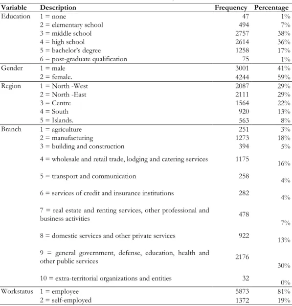
Table 2 shows a description of the variables. All variables present very close values for mean and median, which suggests a normal distribution. The standard deviation is particularly high for the Income variable. Income represents the income of individuals after considering taxes and excluding additional benefits other than personal income. It reaches a minimum of €200 and a maximum €806 000. A minimum value of €200 should not be surprising, even if very low, as it might derive from additional sources of income, not measured by the dataset. The dependent variable of the analysis is the logarithm value of income. The logged value of income presents a notably reduced standard deviation respect to its nominal values.
The description of the binary variables (Gender and Workstatus) shows that are slightly more females than male, and more employees than self-employed. Looking at the categorical variables (Education, Industry, Workstatus and Region) the most common degree are Middle
10 The reason for the exclusion is that unemployment is out of scope for the analysis’ purpose. It is not possible
to analyze regional difference in return to education, if the precondition of being able to support oneself is not met.
School, High School, and Bachelor degree. The most common industry of activity is in public services, followed by manufacturing, retail, and domestic services. Traditional employment is largely preferred to self-employment. The Northern regions have the most inhabitants.
Table 1 - Numerical Variables Description
Table 2 - Dummy Variables Description11
11 The variables take values from 1 on in order to respect the SHIW codebook provided by ISTAT.
Conventionally categorical variables start at 0, but the interpretation does not change.
Description Mean Median St. Dev Min Max
Income after taxes 23912 20280 21415.13 200 806000.0 Logarythm of Y 9.917 9.906 0.5815195 5.298 13.600 Potential experience: Age minus
the year of finishing the highest degree
26.24 27.00 10.33384 -1.00 69.00
Potential experience squared 795.1 729.0 549.1991 0.0 4761.0
Variable Description Frequency Percentage
Education 1 = none 47 1% 2 = elementary school 494 7% 3 = middle school 2757 38% 4 = high school 2614 36% 5 = bachelor’s degree 1258 17% 6 = post-graduate qualification 75 1% Gender 1 = male 3001 41% 2 = female. 4244 59%
Region 1 = North -West 2087 29%
2 = North -East 2111 29% 3 = Centre 1564 22% 4 = South 920 13% 5 = Islands. 563 8% Branch 1 = agriculture 251 3% 2 = manufacturing 1273 18%
3 = building and construction 394 5%
4 = wholesale and retail trade, lodging and catering services 1175 16%
5 = transport and communication 258 4%
6 = services of credit and insurance institutions 282 4% 7 = real estate and renting services, other professional and
business activities 478
7% 8 = domestic services and other private services 922 13% 9 = general government, defense, education, health and
other public services 2176 30%
10 = extra-territorial organizations and entities 32 0%
Workstatus 1 = employee 5873 81%
To test for normality, an Adjusted Jarques-Bera test is performed on the variables, and they are confirmed to be normally distributed, at p-values lower than 2.2e-16. In particular, the test improves for Income when it takes its logarithm value.
The Augmented Dickey-Fuller test is performed to check for the non-stationarity of the dummy variables (Education, Gender, Region, Branch, and Workstatus). They all reject the stationarity hypothesis at 0.01 significance level. In addition, by taking the variables in their dummy forms, and looking at a correlation table not significant correlation was identified such that might generate multicollinearity.
5. Methodology and Empirical Findings
With the purpose of analyzing regional returns to education the Mincer’s equation is used, having as the dependent variable the logarithm of earning, and as independent variables the work experience and the level of education measured by the latest type of degree. The used control variables are the squared value of experience, the gender, the branch of working activity, and the work status (either employees or self-employed). An initial regression has as an additional control variable a dummy for the macro-regions, however, this regression is added for comparison purposes. The main regression is subdividing the data into five sub-sectors, in order to consider each macro-region as being independent. The model can be represented by the following equation:
ln(𝑌𝑖,𝑟) = 𝛽0+ 𝛽1(𝐸𝑑𝑢𝑐𝑎𝑡𝑖𝑜𝑛𝑖,𝑟) + 𝛽2(𝑋𝑖,𝑟) + 𝛽3(𝑋𝑖,𝑟2 ) + 𝛽4(𝐺𝑒𝑛𝑑𝑒𝑟𝑖,𝑟)
+ 𝛽5(𝐵𝑟𝑎𝑛𝑐ℎ𝑖,𝑟) + 𝛽6(𝑊𝑜𝑟𝑘 𝑆𝑡𝑎𝑡𝑢𝑠𝑖,𝑟) + 𝜀𝑖,𝑟
i= year; r=region.
The variables Education, Gender, Branch, and Workstatus are used as dummy variables. For the purpose of the analysis, the dummy = 1 will be removed, in order to avoid the dummy variable trap.
5.1 Empirical Findings
The data in use are unbalanced panel data, they observe 8 variables, collected every second year for 20 years, for 7254 individuals. The regressions were initially estimated by a Generalized Linear Model, using Robust Standard Errors. However, the Breusch-Pagan test for heteroscedasticity identified not constant variances across the error terms. Therefore, the regressions could be better estimated by Heteroskedastic Consistent Standard Errors (also known as Eicker–Huber–White standard error). The Hausman test indicates to use fixed effects in order to account for individual characteristics that are time independent and do not vary over time.
The return to education it is expected to vary according to different macro-regions in Italy. Different models are used to perform the analysis:
• Regression 0 – Regions are included as a control dummy. This regression is performed for comparative purposes and considers the data as a whole.
• Regression from 1to 5 – Differentiated Macro-Regions. Five different regressions are performed, one per each region. Namely, Regression 1 considers the macro-area of North-West, Regression 2 considers North-East, Regression 3 considers the Centre, Regression 4 considers the South, and Regression 5 considers the Islands.
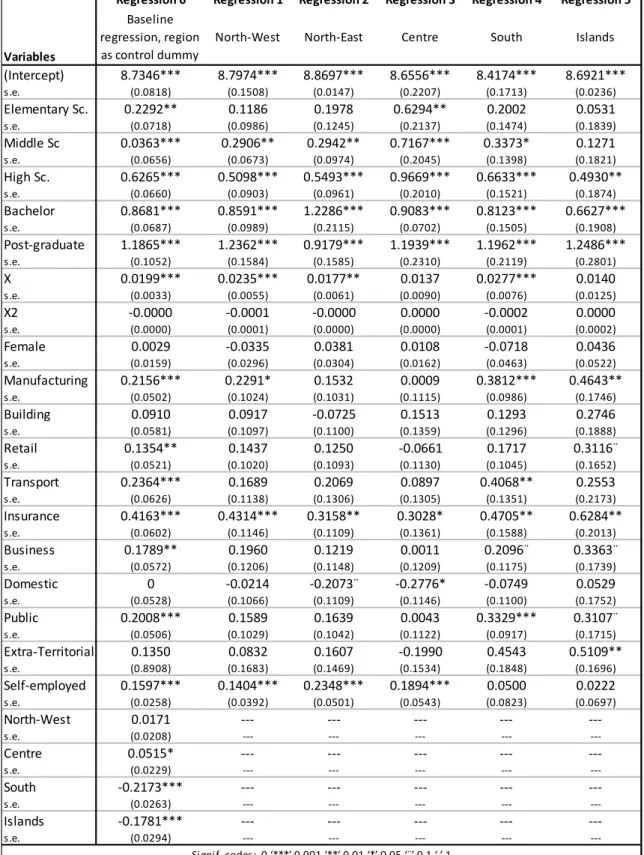
Table 3 - Regression results for different regions, in years 1995-2014. Dependent variable LY
Regression 0 Regression 1 Regression 2 Regression 3 Regression 4 Regression 5
Variables
Baseline regression, region as control dummy
North-West North-East Centre South Islands
(Intercept) 8.7346*** 8.7974*** 8.8697*** 8.6556*** 8.4174*** 8.6921*** s.e. (0.0818) (0.1508) (0.0147) (0.2207) (0.1713) (0.0236) Elementary Sc. 0.2292** 0.1186 0.1978 0.6294** 0.2002 0.0531 s.e. (0.0718) (0.0986) (0.1245) (0.2137) (0.1474) (0.1839) Middle Sc 0.0363*** 0.2906** 0.2942** 0.7167*** 0.3373* 0.1271 s.e. (0.0656) (0.0673) (0.0974) (0.2045) (0.1398) (0.1821) High Sc. 0.6265*** 0.5098*** 0.5493*** 0.9669*** 0.6633*** 0.4930** s.e. (0.0660) (0.0903) (0.0961) (0.2010) (0.1521) (0.1874) Bachelor 0.8681*** 0.8591*** 1.2286*** 0.9083*** 0.8123*** 0.6627*** s.e. (0.0687) (0.0989) (0.2115) (0.0702) (0.1505) (0.1908) Post-graduate 1.1865*** 1.2362*** 0.9179*** 1.1939*** 1.1962*** 1.2486*** s.e. (0.1052) (0.1584) (0.1585) (0.2310) (0.2119) (0.2801) X 0.0199*** 0.0235*** 0.0177** 0.0137 0.0277*** 0.0140 s.e. (0.0033) (0.0055) (0.0061) (0.0090) (0.0076) (0.0125) X2 -0.0000 -0.0001 -0.0000 0.0000 -0.0002 0.0000 s.e. (0.0000) (0.0001) (0.0000) (0.0000) (0.0001) (0.0002) Female 0.0029 -0.0335 0.0381 0.0108 -0.0718 0.0436 s.e. (0.0159) (0.0296) (0.0304) (0.0162) (0.0463) (0.0522) Manufacturing 0.2156*** 0.2291* 0.1532 0.0009 0.3812*** 0.4643** s.e. (0.0502) (0.1024) (0.1031) (0.1115) (0.0986) (0.1746) Building 0.0910 0.0917 -0.0725 0.1513 0.1293 0.2746 s.e. (0.0581) (0.1097) (0.1100) (0.1359) (0.1296) (0.1888) Retail 0.1354** 0.1437 0.1250 -0.0661 0.1717 0.3116¨ s.e. (0.0521) (0.1020) (0.1093) (0.1130) (0.1045) (0.1652) Transport 0.2364*** 0.1689 0.2069 0.0897 0.4068** 0.2553 s.e. (0.0626) (0.1138) (0.1306) (0.1305) (0.1351) (0.2173) Insurance 0.4163*** 0.4314*** 0.3158** 0.3028* 0.4705** 0.6284** s.e. (0.0602) (0.1146) (0.1109) (0.1361) (0.1588) (0.2013) Business 0.1789** 0.1960 0.1219 0.0011 0.2096¨ 0.3363¨ s.e. (0.0572) (0.1206) (0.1148) (0.1209) (0.1175) (0.1739) Domestic 0 -0.0214 -0.2073¨ -0.2776* -0.0749 0.0529 s.e. (0.0528) (0.1066) (0.1109) (0.1146) (0.1100) (0.1752) Public 0.2008*** 0.1589 0.1639 0.0043 0.3329*** 0.3107¨ s.e. (0.0506) (0.1029) (0.1042) (0.1122) (0.0917) (0.1715) Extra-Territorial 0.1350 0.0832 0.1607 -0.1990 0.4543 0.5109** s.e. (0.8908) (0.1683) (0.1469) (0.1534) (0.1848) (0.1696) Self-employed 0.1597*** 0.1404*** 0.2348*** 0.1894*** 0.0500 0.0222 s.e. (0.0258) (0.0392) (0.0501) (0.0543) (0.0823) (0.0697) North-West 0.0171 --- --- --- --- ---s.e. (0.0208) --- --- --- --- ---Centre 0.0515* --- --- --- --- ---s.e. (0.0229) --- --- --- --- ---South -0.2173*** --- --- --- --- ---s.e. (0.0263) --- --- --- --- ---Islands -0.1781*** --- --- --- --- ---s.e. (0.0294) --- --- --- --- ---Signif. codes: 0 ‘***’ 0.001 ‘**’ 0.01 ‘*’ 0.05 ‘¨’ 0.1 ‘ ’ 1
Before starting the analysis, it is a suitable test if the coefficients are statistically different from each other across the various regressions. A Welch-Two Sample t-test was performed considering two regressions at the time, ensuring comparisons across all of them. All the tests rejected the null hypothesis of “the true difference in means is equal to 0”.
5.1.1 Indipendent Variables
The coefficients measuring the return to Education are positive and significant below 0.1% confidence level across all the regressions, for High School, Bachelor, and Post-Graduate. Middle school is significant at different levels across all regressions, except in the Islands. Elementary School is only significant in the overall regression 0 and in the center, both at 0.1% level of significance. The left-out dummy is “Education = none”. Not considering Elementary school, which was not significant, we can see that in the North-West, Center, and South getting an addition degree is constantly increasing the expected return. A similar pattern occurs in the North-East as well, but a Post-Graduate degree, in this case, shows a diminishing return. The islands show increasing return to the level of education, but only from High School on. It was possible not only to confirm the return to education but to also see how its progression increases from one qualification to the other. This result is in line with Brunello, Comi and Lucifora (2000), that for the previous waves of data also found similar results, but only accounting for North and South. The pattern is similar across the regions, but the magnitude is different: The North-West and the South are the two regions showing higher returns to education. Between them, the North-West shows higher returns for the university levels of education, while the South for the secondary school levels. The Islands present the lowest and less significant returns to education. The North-East and the Center present an in-between level of returns. In particular, comparing between the two the North-East has higher returns at the university level, while the Center at the lower levels of education. In accordance with Combes, Duranton and Gobillon (2005) it was possible to explain in the case of Italy that there are differences in return to education and that they vary at regional level. This paper started by looking at differences in income across the country, and simultaneously at the educational results.12 The intuition that education was explaining
parts of the regional differences in returns was quantified in the empirical section.
The work experience X is significant at below 0,1% confidence level in the overall regression, in the North-West, and in the South. It is significant at 0,1% in the North-East and insignificant in the Centre and the Islands. One extra year of experience increases the expected income by 2% in the North-West and in the South, and of 0,2% overall and in the North-East. As expected form Mincer’s equation (1974), it is possible to see that the work experience is positively related to earnings, and it varies across regions.
5.1.2 Control Variables
The squared work experience X2 is surprisingly not significant in any case. The coefficient is generally negative, except in the Center and in the Island. The general negative coefficient confirms the assumption made in the depiction of Mincer’s equation (1974) of diminishing returns: one individual is more likely to get significant promotions and step further in his career when he is less experienced and at the beginning of his career. The positive coefficient for the Center and in the Islands, might open up for further investigation. These two regions, did not show a significant relationship between experience and earnings not even in the case of linear experience X. Furthermore, the Islands presented the weakest return to education as well. It might be worth investigating if there are increasing returns at all in these regions, and what are the caused by, if not education and experience.
The dummy for Gender is not significant in any case. However, additional analyses might be performed on this interesting finding, as it seems to suggest that there is not gender disparity in earnings. Most likely this is related to the particular dataset in use, as it only accounts for single households. Further speculation should be made assessing if for a female having or not having a family (namely, not being in a single household) has an impact on her career. The left-out dummy is “Gender = male”. These finding are not in line with the results of Lucifora and Meurs (2006). Their study considered the same data, but with a different research question, focused on gender pay gap. Their explanation of the existence of the pay gap consider the further subdivision of public vs. private sector and low skilled vs. high skilled between male and female. In other words, women are mostly low skilled and in the public sector, and this result in them earning less than male.
The dummies for Branch are control variables, the excluded dummy is “Branch = Agriculture”. Their coefficients of the included dummies are mostly insignificant. The exception are the dummy for Insurance, significant at different levels across all the
regressions; and the dummy for Manufacturing, significant at different levels across all the regressions except in the North-East and in the Center. They both present positive coefficients, indicating that they might be better working areas than Agriculture. This is in line with the Krugman (1991) from the distinction between Agriculture and Manufacturing. It also adds a third sector, Insurance, that can also be considered high-skilled compared to Agriculture. Krugman (1991) takes Agriculture and Manufacturing as baselines examples for low-skilled and high-skilled, so Insurance could be considered as part of high-skilled jobs as well.
The work status it is a dummy, used as a control variable, that excludes “Workstatus = employee”, and therefore accounts for self-employment. Before the analysis, the unemployed individuals were excluded as well, as they cannot present return to education if they do not perceive any income deriving from their own work. The coefficients are positive and the significances below 0,1% confidence level in all the regions, except the South and the Island, where it is not significant at all. This points in the direction of further investigation in relation to entrepreneurial activity and the North-South gap as explained by Brunello, Comi and Lucifora (2000). As anticipated in the variables description section, there is not a clear effect of return entrepreneurship across different countries. The same reasoning can apply across the Italian regions. (Namatovu & Dawa, 2017; Pascual & Martin, 2017) The Northern regions of them appear to be sensitive to differences in return to entrepreneurial activities and the Southern not. Further research is needed to assess with the clarity the Italian case on this topic.
When studying the dummies for regions in the baseline model 0 we can see that wages are lower in the South and the Islands compared to the North-West, although controlling for education. This might signal that the difference between the North (West) and South (and Islands) may be due to other factors than differences in return to education.
6. Conclusion
The main conclusion from this empirical analysis is that there are differences in return to education across the Italian macro-regions. In general, in each region an additional degree increased the expected return more than the previous degree did.
Accounting for degree level, the North-West and the North-East perform better when considering the return to higher education, while the South and the Center presents higher returns when accounting for lower levels of education. The Islands do to present highly significant returns to education. This is in line with the expectations that the North overall is richer than the South overall, as higher degrees guarantee higher returns. The regions presenting overall the highest returns are the North-West and the South, surprisingly as the North-South gap debate lead to the expectation that the South will always underperform. The findings of the current study do not, however, contradict the previous literature about the North-South gap. In facts, they offer more insights by decomposing these differences even further. Not necessarily if the South (intended as South +Island +part of the Center) lags behind the North (intended as North-West +North-East + part of the Center) all the parts of the South lag behind all the part of the North.
A surprising finding came from the work experience. In its linear term, it was proven positively related to income, as expected. However, its squared term was generally insignificant, which contradicts the expectation of diminishing return over time.
Policy recommendation should regard the main results: the differences in return to education across regions. In order to arrive at a homogeneous standard across the entire country the North-East and North-West could invest more in lower level education. At the same time, however, as are the higher levels of education that guarantee the higher returns, these two regions might keep their current spending levels and continue nurturing their competitive advantage in higher education. The decision regards the perspective of equality versus specialization. The Centre and South, vice versa, should increase their focus on higher level education. In these cases, however, this is the only choice. There is no incentive in developing a competitive advantage in a sector that is not the most fruitful one. The Islands are showing high returns to post-graduate education. They should focus on all the other lower levels of educations. Another way might be keeping the focus on post-graduate studies, while working
on attracting talents from the other regions for this qualification in particular. A caveat of the current analysis is that internal migrations are disregarded, so this recommendation might already be in place, but uncaptured by the data.
Further research should take as primary variables the control variables used in this study. The consideration of only the single households might be a good explanation for the non-gender biased results, and for the insignificance of decreasing returns to work experience, but this should be analyzed in practice before making any speculation. Moreover, the control variable for entrepreneurial activity seems to suggest that returns might be different between Northern and Southern regions, additional analyses should go in this direction.
7. Limitations
The results of this study were obtained under some assumptions and limitations to the analysis. The most considerable limitation was the fact that the data in use accounted solely for single households, not considering families composed by more than one working age member. This allowed to account for individual characteristics such as level of education and working industry, but excluded a substantial part of the data. An additional limitation was the impossibility of accounting for migration effects, and to check if an individual is working in the same regions where he studied. As the sample used was sufficiently large, the analyses were produced under the assumption that the internal migration effect was small enough to be neglected. This is an uncertain assumption, and individual’s location choice should be subject of further studies for a more complete picture of the situation.
8. References
Agasisti, T., Ieva, F., & Paganoni, A. (2017). Heterogeneity, School-Effects and the North-South Achievement Gap in Italian Secondary Education: Evidence FRom a Three-Level Mixed Model. Statistical Methods & Applications, 157-180.
Backman, M., & Bjerke, L. (2009). Returns to Higer Education - a regional perspective. CESIS
Electronic Working Paper Series No. 171, 1-30.
Becker, G., & Tomes, N. (1986). Human Capital and the Rise and Fall of Families. Journal of
Labour Economics 4(3), 1 - 39.
Behrens, K., Duranton, G., & Robert-Nicoud, F. (2013). Productive Cities: Sorting, Selection and Agglomeration. Working Paper Series WPS 13-11-1.
Brunello, G., Comi, S., & Lucifora, C. (2000). The Returns to Education in Italy: A New Look at the Evidence. IZA Discussion Paper No. 130, 55.
Cannavale, A. (2015). Divario Nord-Sud: tutto iniziò con l’Unità d’Italia. L’incapacità ‘genetica’
non c’entra. Retrieved from Il Fatto Quotidiano:
http://www.ilfattoquotidiano.it/2015/03/25/divario-nord-sud-tutto-inizio-con-lunita-ditalia-lincapacita-genetica-non-centra/1535817/
Caplan, B. (2006). Two Educational Heresies: Ability Bias vs. Signaling. Retrieved from Library
of Economics and Libery:
http://econlog.econlib.org/archives/2006/06/two_educational.html Card, D. (1994). Earnings, schooling and ability bias revisited.
Cavallaro, C. (2014). Regional Geography. In S. Mangiameli, Italian Regionalism: Between
Unitary Traditions and Federal Processes (ISBN 978-3-319-03764-6 ed., pp. 81 - 109).
Springer International Publishing Switzerland. doi:DOI 10.1007/978-3-319-03765-3 Cieslik, A., & Rokicki, B. (2016). Individual Wages and Regional Market Potential. Economics of
Transition, 661-682.
Combes, P., Duranton, G., & Gobillon, L. (2005). Spatial Wage Disparities: Sorting Matters!
Journal of Urban Economics 63, 723-742.
Cowen, T., & Tabarrok, A. (2011). Modern Principles of Economics. Worth Publishers.
Currid, E. (2010). How Art and Culture Happen in New York. Implications for Urban Economic
Development, 454-467.
Deschenes, O. (2001). Unobserved Ability, Comparative Advantage, and the Rising Return to Rducation in the United States 1979 - 2000.
Docampo, D., & Cram, L. (2017). Academic Performance and Institutional Resources: A Cross-Country Analysis of Research Universitities. Scientometrics 110, 739-764.
Duranton, G., & Puga, D. (2004). Micro-foundations of urban agglomeration economies.
Handbook of regional and urban economics 4, 2063 - 2117.
Ellickson, B. (1971). Jurisdictional Fragmentation and Residential Choice. American Economic
Review 61, 334-339.
ENQA. (2017, April 17). European Association for Quality Assurance in Higher Education. Retrieved from ENQA: http://www.enqa.eu/
Fally, T., Paillacar, R., & Terra, C. (2010). Economic Geography and Wages In Brasil: Evidence From Microdata. Journal Of Development Economics 91, 155-168.
Feldman, M. (1994). Knowledge complementarity and innovation. Small Business Economics 6, 363-372.
Florida, R. (2012). The rise of the creative class - Revisited Edition. Basic Books; 2 edition. Friedman, M. (1962). Capitalism and Freedom (ISBN 0-226-26421-1 ed.). University of Chicago
Press.
Galor, O., & Zeira, J. (1991). Income Distribution and Macroeconomics. The Review of Economic
Studies. Oxford: Oxford University Press., 35-52.
Girliches, Z. (1977). Estimating the Returns to Schooling: Some Econometric Problems.
Econometrica 45, 1-22.
Glaeser, E. (2005). Review of Richard Florida’s The Rise of the Creative Class. Regional Science
and Urban Economics 35 (5), 593 - 596.
Gpg Imperatrice. (2012). L’Apocalisse Meridionale: il SUD e’ il problema (ed opportunita’)
numero 1 dell’Italia. L’Italia e’ MORTA se non si affronta questa questione. Retrieved
from Rischio Calcolato: https://www.rischiocalcolato.it/2012/09/lapocalisse-