Comparison of angular measurements by 2D and 3D gait analysis

(1)

Comparison of angular measurements

by 2D and 3D gait analysis

Dennis Brandborg Nielsen

Marika Daugaard

Thesis, 15 HP

Orthopaedic technology

Jönköping, spring 2008

Supervisor: Lee Nolan Ph.d., University lector Examiner: Dan Karlsson, Ph.d.

___________________________________________________________________________ School of health sciences, Jönköping University

(2)

Abstract

Objective: To validate the use of a 2-dimensional video based system (Hu-m-an digitizing

software, HMA Technology Inc. Ontario, Canada), for measuring sagital plane knee and ankle angles during gait analysis.

Design: Criterion-based, concurrent validation. Participants: 18 persons without any gait disorders.

Method: The participants were subjected to simultaneous capture of their motion data with a digital

video camera filming in the sagital plane only, and a 3-dimensional optoelectronic motion capture system (Qualisys Medical AB, Gothenburg, Sweden). The data was analyzed both using Hu-m-an digitizing software (HMA Technology Inc. Ontario, Canada) and Visual 3D (C-motion Inc., Kingston, Canada) respectively.

Outcome: Relative angles for the knee and ankle.

Results: Significant difference was found between the systems for measuring ankle angles

(p<0,05). No significant difference was found for measuring knee angles at stance, but significant differences was present during swing and at IC (p<0,05).

Even though significant differences were found, the correlation, between the two systems, was high for the knee, and moderate to high for the ankle.

Conclusion: Hu-m-an digitizing software (HMA Technology Inc. Ontario, Canada) has been

demonstrated to be a promising tool for measuring 2-dimensional sagital plane knee and ankle angles, but cannot be validated from this study alone.

Keywords: Gait measurement, validation, 2-dimensional analysis, 3-dimensional analysis,

(3)

Sammanfattning

Målsättning: Att validera användningen av ett 2-dimensionellt videobaserat system (Hu-m-an

digitizing software, HMA Technology Inc. Ontario, Canada), för att mäta knä- och ankelvinklar i sagittalplanet under gång.

Design: Criterion-based, concurrent validation. Deltagare: 18 personer utan gångproblem.

Metod: Deltagarens rörelsemönster mättes av en digital videokamera som filmade i sagittalplanet

och av ett 3-dimensionellt optoelektroniskt rörelsesanalyssystem (Qualisys Medical AB, Gothenburg, Sweden) samtidigt. Data analyserades genom att använda både Hu-m-an digitaliseringsmjukvara (HMA Technology Inc. Ontario, Canada) och Visual 3D (C-motion Inc., Kingston, Canada).

Undersökta parametrar: Relativa vinklar för knä och ankel.

Resultat: Signifikant skillnad observerades mellan systemen vid mätning av ankelvinkeln (p<0,05).

Ingen signifikant skillnad observerades vid mätning av knävinklar i ståfasen, men signifikant skillnad observerades i svingfasen och vid hälkontakt (p<0,05).

Även om det fanns en signifikant skillnad var korrelationen mellan de två systemen hög för knäet, och moderat till hög för ankeln.

Konklusion: Hu-m-an digitaliseringsmjukvaran (HMA Technology Inc. Ontario, Canada) tyder på

att vara ett lovande verktyg för att mäta 2-dimensionella knä- och ankelvinklar i sagittalplanet, men kan inte valideras enbart ifrån denna studie.

Nyckelord: Gång mätningar, validering, 2-dimensionel analys, 3-dimensionel analys, digitalisering,

(4)

Introduction

Gait analysis is performed on a routine basis by clinicians all around the world. The most common method for gathering gait analysis data is to do an observational gait analysis (OGA). Nowadays the demand for evidence based practice is increasing, and since OGA is a subjective method of analyzing, it conflicts with the demand for validated results.

A known validated method for gait analysis is 3-dimensional optoelectronic motion analysis. The systems used to perform such an analysis are comprehensive, often expensive and more commonly used for research. They are seldom used in clinical practice, first and foremost because of the cost, secondly since it is time demanding and impractical, and thirdly the personal operating the system has to have a thorough education and experience to operate the system.

What clinicians are looking for is an analysis method that can aid them in improving the OGA, but still be practical to use in a clinical setting. It should be able to quantify gait data and be validated. Video-based 2-dimensional motion analysis systems are recognized as a useful tool for gait analysis. It does not require an as in-depth knowledge as 3D systems, and the equipment used is commonly available and reasonably cheap. To the authors knowledge there have been few studies concerning clinical validation of 2D video-based motion analysis, of which there are several different systems, so the use of it as the basis for evidence-based decision making can be questioned.

The aim of this study was to validate Hu-m-anTM_{video-based 2D analysis (HMA Technology Inc.}

Ontario, Canada), by comparing simultaneous measurements with the 3D motion analysis system: Qualisys Tracking Manager (Qualisys Medical AB, Gothenburg, Sweden).

Randomily selected sagital plane relative angles for the knee and ankle during gait were analyzed, as well as the angles at initial contact.

Background

There are different opinions among clinicians on the value of gait analysis as a clinical tool. The relevance of a basic gait analysis, for assessing the patient with gait disorders in a clinical setting, is generally recognized. The discussion revolves around whether the methods for clinical application should be validated in the same way as those used for research, and if using 3D analysis outside research projects is beneficial (Baker, 2006).

(6)

Baker (2006) states that the criterion for valid clinical research is not the same as that for clinical testing. In clinical testing there is only one subject, and random errors within the test can influence the results and make them unreliable. By increasing the number of subjects for research purposes, the effect of the random errors can be reduced and allow for meaningful conclusions. This fact influences the validity of using gait analysis in clinical practice.

The areas of interest, for which data can be collected, are kinetics, kinematics and dynamic EMG (Barker, Craik, Freedman, Herrmann & Hillstrom., 2006). The variables most often analyzed are kinematic variables (Smidt, 1974). Though kinematic results are more easily interpreted, it must be noted that it only describes a patient’s movement, whereas kinetics can determine the cause of the movement. Sagital plane kinematics are more reliable than frontal and transverse, particularly angle measurements for the larger joints such as hip and knee, compared to the measurements for the ankle (Krebs, Edelstein & Fishman, 1985; Kadaba et al., 1989). With modern technology quantification of motion data is now easier. The results are not intended to form the basis of medical diagnostics, but instead aid in choosing the appropriate intervention for patients with gait disorders, and assess the outcome of the intervention (Simon, 2004).

The most utilized type of gait analysis is OGA, but Krebs et al. (1985) found the reliability of observational kinematic gait analysis to be only moderate at best. Even though the clinical settings for this study provided better terms for doing an accurate and repeatable analysis, than would be encountered in practice, and the clinicians had considerable experience, the reliability was still lower than expected.

Coutts (1999) states that OGA is insufficiently reliable and should not be used on its own, unless done by a clinician with a high level of expertise. The analyses should be supplemented with some sort of objective test to get a reliable measure. Videotaping the gait allows for repeated viewing, slow motion and freezing of a specific frame, which will improve the reliability of OGA.

The demand for evidence based practice is increasing with the added pressure from the authorities on the clinicians to state the cost and quality of life ratio, before reimbursement of intervention will be approved (Nielsen, 2002). The arguments for reimbursement should be based on well defined research publications, and the methods for assessing the patients need to be validated, to ensure that the result can be trusted as a base for a treatment plan.

Optoelectronic 3D motion analysis systems have been validated as a patient assessment tool, but still have their limitations (Richards, 1999). One of the major limitations to the systems is the need for applying skin markers on the patient. The placement of the markers has an influence on the

(7)

kinematic results (Kadaba et al., 1989; Kadaba, Ramakrishnan & Wootten, 1990). The markers are placed manually based on anatomical landmarks palpated at application. Differences can occur between different clinicians applying the markers on the same patient (inter-class correlation), and also between applications done by the same clinician (intra-class correlation) (Kadaba et al., 1990). Since the markers are placed on the skin, their movement is influenced by the movement of the soft tissue underneath. Benoit et al. (2006) did a study determining the effect of skin movement on the kinematics for the knee joint during gait, by comparing skin markers to pin in bone markers. They found that although the skin markers could provide repeatable results, it could not be compared with the kinematics retrieved from the pin in bone analysis. Therefore kinematic analysis is prone to errors resulting from the movement of the soft tissue, and this should be considered when interpreting kinematic data.

The major reason that 3D optoelectronic gait analysis are not used more frequently in clinical practice, even though it has been proven to be a valid method of testing, is the time and expense factor. It is a considerable investment to purchase the equipment and very few clinics can afford it. The gait analysis system must pay for itself within a reasonable time span. This is often only possible if the gait laboratory runs full time, which is rarely manageable in practice. Therefore gait laboratories are often regarded as inefficient, unproductive, and uneconomical (Simon, 2004). An alternative method for quantifying gait analysis data is to use 2D video-based motion analysis. It is a simpler and less expensive analysis method, where all that is required is a digital video camera, and a digitizing software program that can be bought at a reasonable price. For these reasons 2D video-based motion analysis is being used more frequently in clinical practice. The issue with 2D analysis is whether or not it can be validated for clinical use.

Churchill, Halligan & Wade (2002) did a study validating the use of the Rivermead video-based clinical gait analysis method (RIVCAM), which is based on the principle of 2D video-based motion analysis. Among others they tested the accuracy of angle measurement of a fixed angle, approximately 69°-70°, that is moved along a walk line, and found a standard deviation (SD) of 0,46°. Finally three illustrative trials were analyzed; one from a “normal” subject, and two from a hemiplegic subject before and after orthotic intervention. This was done in order to try and assess the utility of the system in clinical practice. The results were promising but the significance can be discussed since the number of subjects was limited.

When working with 2D there are a couple of things that need to be considered. One is the phenomenon of parallax error, which occurs when objects are viewed away from the optical axis of

(8)

the camera. This error can be minimized by aligning the optical axis with the center of the motion (Kirtley, 2006). Another thing is perspective errors, or out-of-plane errors. These occur when the object is moving out of the calibrated plane, where the actual size of the object is known. If the object moves closer or farther away from the camera, than the distance to the calibrated plane, the presumed size will be incorrectly measured (Sih, Hubbard & Williams, 2001).

Errors can occur in the measurement of angles, if an analysis is performed on a transversal rotation, where the limb rotates out of the plane, e.g. a cerebral palsy child with excessive femoral rotation. Mathematical corrections can be implemented to correct this error but Stevens, Schmitt, Cole and Chan (2006) stated that for transversal rotations, less than 20° out of plane, it is not recommendable to make this adjustment. Correction of this error does not result in significant different outcomes than the non-adjusted outcomes.

This study examines criterion-based, concurrent validity by simultaneous gait analyses with 2D video-based Hu-m-an digitizing software (HMA Technology Inc. Ontario, Canada) and a 3D optoelectronic system: Qualisys Tracking Manager (Qualisys Medical AB, Gothenburg, Sweden). The criterion measurement system is the Qualisys Tracking Manager.

Method

Subjects

18 subjects, 8 males and 10 females, were recruited for the study at Jönköping University. The subjects were included on the criteria that they did not have any pathological symptoms influencing their gait. The mean age was 24,72 years (SD 1,96 years), mean height was 173,50 cm (SD 9,03 cm) and mean mass was 66,94 kg (SD 10,20 kg).

Prior to the study a student’s ethical consent form was filled in. The subjects were informed orally about their rights and the ethical consideration concerning this study before any testing began. They were allowed to leave the study at any time and their anonymity was ensured.

Equipment and testing protocol

Testing was performed in the Biomechanics laboratory at the school of health sciences, Jönköping University. The subjects were asked to walk at a self-selected walking velocity along a 10 m

(9)

walkway while being recorded by both the 2-dimensional and 3-dimensional system. The direction in which the subjects walked was randomized.

The 3-dimensional optoelectronic motion data was recorded using eight motion capture cameras, ProReflex 120, with a recording speed of 100 Hz. The data was collected using Qualisys Tracking Manager (Qualisys Medical AB, Gothenburg, Sweden).

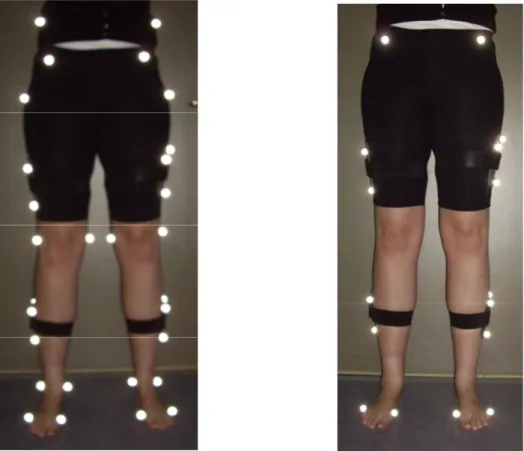
Before testing the system was calibrated to less than 1,5 mm in error of length, within a calibration area of 3m x 1,2m x 0,7m, which corresponds with the area where the 2D analysis should be performed. The subjects were fitted with reflective markers on the lower limbs according to the cluster marker model (see Figure 1). See appendix I for detailed information.

Figure 1: Placement of the reflective markers for lower limb gait analysis. Marker setup for static analysis is seen to the left, and setup for dynamic analysis is seen to the right. On the thigh and shank, clusters with 3 reflective markers are applied, which defines the segments movement in space.

In order to capture a video sequence for 2-dimensional analysis, a digital video camera (Canon XM2 PAL Mini, Canon Inc., Tokyo, Japan) was set up so that it could record the subjects in the sagital plane. The camera was placed on a level tripod, perpendicular to the center of the pathway at a distance of 3 meters, and 55 cm above the floor (see Figure 2). Since it was the lower limb that

(10)

was to be analyzed, the camera was set in this height so that the optical axis of the camera was aligned with the knee. Any changes of the picture related to the shape of the standard lens (Canon Professional L-series Fluorite Lens, Canon Inc., Tokyo, Japan) would then be evenly distributed over the thigh and shank. This setting ensured that the calibration area covered the lower limb. The camera was set to view 3 of the 10 meters of the walkway. The gait was captured in 25 Hz with a shutter speed of 1/1000 seconds.

For the video, a 1,2m 2D vertical calibration frame was recorded in five different positions one in the center of the calibration area and two to each side, 50 cm apart. The total calibration volume was therefore 2m x 1.2m. The system was not calibrated in depth, as Qualisys was, but only as an 2-dimensional plane aligned with the pathway (see Figure 2).

The two systems were synchronized frame to field by the use of a custom build device that rotates a stick consisting of a reflective marker and an arrow (see Figure 3).

Figure 3: Custom build synchronization device with a reflective marker and

arrow on a rotating stick. 3m

2m

1,2m

Axis of rotation

Arrow lined up with top of triangle (detected by video) at the same point as the reflective marker is at its lowest point (detected by ProReflex 120)

(11)

These could be observed by both systems and could determine a specific point in time where the arrow was both vertical i.e. pointing to the top of the triangle, and the marker at its lowest position. The stick rotated approximately 1,4° per field. The goal was to adjust the speed so that it was slow enough to capture a field with the arrow close to the top of the triangle, but fast enough so that a change in position could be observed. The sampling rates are 50 fields/s for Hu-m-an and 100 frames/s for Qualisys, so the maximum synchronizing error, as the position of the arrow with respect to the triangle could be clearly seen in each field, would be 1/50 second (0,02 s).

Analysis

After gathering the recordings they were analyzed using two different methods.

The ProReflex cameras, in collaboration with Qualisys, automatically tracked the reflective markers, which then had to be visually inspected by the authors and exported into a format that could be interpreted and analyzed by Visual 3D (C-motion Inc., Kingston, Canada).

Before analyzing the 2D motion data, captured by the digital video camera, the video sequences was deinterlaced using EditV32 (HMA Technology Inc. Ontario, Canada), so that the 25 frames became 50 fields. The video sequences were then analyzed using Hu-m-an digitizing software (HMA Technology Inc. Ontario, Canada).

The frames/fields were renumbered so that zero in the ProReflex data was the point of the lowest marker position from the synchronization unit, and zero in the video fields was the point where the arrow was at the top of the triangle.

10 fields were then randomly selected to be analyzed, within the time frame where the limb in question was fully visible in the video sequence. In order to make sure the same 10 fields/frames were chosen in both analysis systems, it was first determined from video which fields were to be analyzed, and then the video field number (50Hz) was transformed into the corresponding frame number in the 3D system (100Hz), by multiplying it with 2.

Visual 3D uses a segmental method for determining joint angles, where the center of rotation is located automatically within the program. The program calculates the joint angles by the means of a decomposition matrix based on Cardan sequences and a 6 degrees of freedom model. The default setting in Visual 3D is to calculate all angles using this method (C-motion Inc., 2002). The decomposition matrix describes the relationship between two local coordinate systems, one for each segment between which the relative angle is determined. The movement of a joint is generally

(12)

considered as the movement of the distal segment in relation to the adherent proximal segment; e.g. for determining the knee angle, the thigh would be the proximal segment and the shank the distal. Movement occur around 3 different axis which describes two definition of movement each: flexion/extension, abduction/adduction, internal/external rotation (Hamill & Selbie, 2004).

The angles chosen for this analysis were knee flexion/extension, determined from the thigh and shank segments, and ankle plantar and dorsi flexion determined by the shank and foot segments. For stating the ankle angles, zero was set at 90° to elucidate what is plantar flexion and what is dorsi flexion. Plantar flexion was set as the negative degrees.

The data were then filtered using a Butterworth second order filter, the Visual 3D default filter, with a cut-off frequency of 6 Hz.

When digitizing manually in Hu-m-an the lower limb was viewed as three segments, thigh, shank and foot. The relative angle is defined as the angle between two lines drawn through the segments. First, the absolute angle from a vertical line (l) to the line of the proximal segment is calculated (θap). Secondly the absolute angle from vertical to the distal segment is calculated (θad), and finally

the difference between these are determined and defined as the relative angle (θr) (see Figure 4)

(HMA Technology Inc., 2005).

The center of rotation for the hip, knee and ankle, identified by one author from video when manually digitizing, were used to define the thigh and shank segments, between which the relative angle for the knee was calculated (see Figure 5).

For determining the relative ankle angle, the shank segment was defined by the center of rotation for the knee and ankle, and the foot segment was defined between the back of the heel and the ball

θ_ad l

θ_ap

θ_r Figure 4: Illustration of relative angle calculation in Hu-m-an.

(13)

of the foot (see Figure 6). For calculations, zero was also set at 90° to elucidate what is plantar flexion and what is dorsi flexion. Plantar flexion was set as the negative degrees.

A filter can be implemented in the analyses with Hu-m-an when digitizing full sequences, more than 20 consecutive fields. The type of filter used is optional and could be chosen to match the one used by Visual 3D. However when digitizing separate fields, the data is not filtered.

The effect of filtering must be considered, to assess whether not implying filtering in Hu-m-an, when a filter is used in Visual 3D, could influence the results of this study. The type of filter used in Visual 3D is a Butterworth second order with a cut-off frequency of 6 Hz. A full gait cycle sequence of 60 fields was digitized for one subject and the angles with and without filtering was compared. A high correlation was present for both knee (rsp = 0,995, p<0,01) and ankle angles (rsp =

0,965, p<0,01). Since the correlation is so high any error related to not using a filter for the Hu-m-an data would be insignificHu-m-ant compared to other errors, such as trHu-m-ansversal rotation of the limb. Thus the method of digitizing a single field, without filtering, was used when reporting the angle data calculated in Hu-m-an.

Relative knee and ankle angles were then determined at several instances during the gait cycle in order to compare the measurement of these angles between the 2 systems. These were at a) a

Figure 6: Illustration of the digitizing method for deter-mination of the relative angle of the ankle in Hu-m-an.

Figure 5: Illustration of the digitizing method for

(14)

random angle chosen during the whole gait cycle at one particular field of the video, and the corresponding frame from the Proreflex system, b) the point of initial contact (determined in the video sequence as the first field with contact between the heel and the floor, and determined in the proreflex data as the corresponding frame).

The data from a) was sorted into two groups; c) random angles chosen during the stance phase at one particular field of the video, and the corresponding frame from the Proreflex system and d) random angles chosen during the swing phase at one particular field of the video, and the corresponding frame from the Proreflex system.

These angles were then statistically compared between the two analysis systems.

Statistical analyses

All statistical analyses were carried out using SPSS software (SPSS for Windows, Rel. 14.0.0 2005, Chicago, SPSS Inc.) with a significance level of α = 0,05.

The data was explored to determine whether or not it was normally distributed using a Shapiro-Wilk test (α = 0,05). The four main groups were the knee and ankle angles values for both Hu-m-an and Visual 3D. None of these data sets were normally distributed. The data sets for angles at IC, stance and swing were also tested for normal distribution. It was found that the data for initial contact was normally distributed for both systems, but the data for stance and swing were not. To be conservative it was chosen that all statistical analyses should be carried out using non-parametric tests.

Wilcoxon signed-rank tests were used to determine statistical significant differences between the data from Hu-m-an and Visual 3D. Spearman correlation tests were used to establish the correlation between Hu-m-an and Visual 3D data. All correlation coefficient interpretation was done according to Franzblau (1958) (see appendix II). Bland-Altman plots were used to visualize the distribution and relationship of the data (Bland & Altman, 1986).

In this study all digitizing was performed by the same author so there is no need to consider intra-correlation. Digitizing error was tested by the same author re-digitizing the same fields on two different occasions and comparing the results using a Spearman correlation test.

(15)

Results

Relative knee and ankle angles randomized during gait

The Wilcoxon signed-rank test proved that there was no statistical significant difference between Hu-m-an and Visual 3D, for determining relative flexion and extension angles of the knee during level gait (z = -1,106, p>0,05). In addition the correlation between knee angles determined by the Hu-m-an and Visual 3D systems was high (rsp = 0,915, p<0,05). The mean difference between the

two systems was -0,29° (SD = 4,05°).

For the determination of the ankle angles using the Hu-m-an and Visual 3D systems there was a significant difference between the two methods (z = -11,626, p<0,05). Even though there was a difference, the significant correlation was high (rsp = 0,806, p<0,05). The mean difference in ankle

angle was 17,52° (SD = 5,39°), where Visual 3D generally measured larger relative angles between the foot and the shank.

For mean and standard deviations (SD) see Table 1.

Table 1: Mean and SD for knee and ankle angles during gait (n = 180). Mean knee angle Mean ankle angle Hu-m-an 161,78° (SD 18,05°) -1,11° (SD 9,49°) Visual 3D 162,07° (SD 18,46°) -18,63° (SD 8,02°)

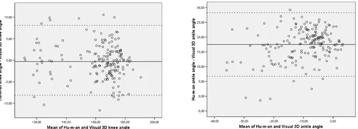
The Bland-Altman plot visualizes whether or not the differences between the two methods differ, depending on the size of the angle that is measured. It showed difference for neither the knee nor ankle (see Figure 7).

(16)

Angles at Initial contact (IC)

At IC the Visual 3D system measured significantly larger knee angles (z = -2,461, p<0,05) and larger ankle angles (z = -3,724, p<0,05) than the Hu-m-an system. Mean and standard deviations are shown in Table 2. There was a -2,21° (SD = 3, 22°) mean difference for the knee angles, and a 24,22° (SD = 3,51°) mean difference for the ankle angles between the 2 systems used. The correlation between the systems was high for the knee and moderate for the ankle (see Table 5).

Table 2: Mean and SD for knee and ankle angles at IC (n = 18).

Mean knee angle Mean ankle angle Hu-m-an 172,57° (SD 4,81°) 1,61° (SD 4,52°) Visual 3D 174,78° (SD 4,95°) -22,60° (SD 3,76°)

Angles during stance

During stance the relative angles for the ankle showed a significant difference (z = -9,779, p<0,05) between the two systems. Again the Visual 3D system was measuring larger relative angles compared with Hu-m-an. The relative knee angles measured during stance showed no difference (z = -0,330, p>0,05) between the two systems. The mean difference for the knee was 0,14° (SD = 3,77) and 18,28° (SD = 4,76°) for the ankle. Correlation was high for the knee and marked for the ankle (see Table 5).

For mean and SD see Table 3.

Table 3: Mean and SD for knee and ankle angles during stance (n = 127). Mean knee angle Mean ankle angle Hu-m-an 168,60° (SD 8,56°) 1,07° (SD 8,25°) Visual 3D 168,46° (SD 9,42°) -17,21° (SD 7,97°)

Angles during swing

During swing there were significant differences between the 2 systems used for both measuring of the relative knee (z = -2,386, p<0,05) and ankle angles (z = -6,281, p<0,05). The mean difference

(17)

for the knee was -1,32° (SD = 4,54°), and for the ankle 15,70° (SD = 6,35°). Even though these differences exist, the correlations were still high (see Table 5).

For mean and SD see Table 4.

Table 4: Mean and SD for knee and ankle angles during swing (n = 53). Mean knee angle Mean ankle angle Hu-m-an 145,45° (SD 23,63°) -6,33° (SD 10,29°) Visual 3D 146,76° (SD 24,90°) -22,03° (SD 7,12°)

Table 5: Spearman correlation coefficient for the six conditions with specification of the significance level.

IC (n = 18) Stance (n = 127) Swing (n = 53) Knee rsp = 0,808 (p<0,05) rsp = 0,846 (p<0,05) rsp = 0,955 (p<0,05)

Ankle rsp = 0,577 (p<0,05) rsp = 0,766 (p<0,05) rsp = 0,816 (p<0,05)

Intra-class correlation

Three subjects were digitized two times, on two different occasions by the same author. The fields that were to be digitized were chosen on the same criteria as for testing; 10 random fields during the entire gait cycle and the one field at IC. The correlation between the result from occasion 1 and occasion 2 was high for both the knee (rsp = 0,990, p<0,05) and ankle angles (rsp = 0,810, p<0,05).

Discussion

Results

The original aim of this study was to validate the use of the 2D video-based motion analysis system Hu-m-an, for measurement of knee and ankle angles in the sagital plane during normal, level gait. When analyzing the data as a whole (n = 180) there proved to be no significant difference between the two systems. However, when the data was analyzed according to specific periods in the gait cycle, there proved to be a significant difference for measuring knee angles during swing and at IC. The mean difference was small, -1,32° in swing and -2,21° at IC, at the same time as the correlation

(18)

was high for both. This indicates that the small error is consistent, but whether it is due to the author’s consistent underestimation of the angle or differences in calculation between the two systems is unclear. Further more the effect of the consistent error can more easily be determined as significant when the groups are small.

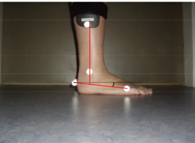
The results showed a significant difference between the two systems when measuring relative ankle angles. This result might be explained by an error related to the marker setup for the 3D analysis. The foot segment is defined by three markers, located on the first and fifth metatarsal head and on the heel. If the heel marker is not placed in the same height as the forefoot markers, when the subject is standing, the system will interpret it as if the foot is angled in either dorsi or plantar flexion. The most common error is that the heel marker is placed too high in relation to the forefoot markers, to avoid that the marker strikes the ground when walking. This results in a plantar flexion degree being measured, when in reality the foot is placed in a neutral position (see Figure 8). The corresponding significant difference and high correlation between the results for the ankle measurements indicates that this error could be present in this study. Visual 3D generally measures higher values than Hu-m-an with a mean difference of 17,52°, which indicates that the static marker setup for the foot segment is generally in about 17° plantar flexion. The mean difference changes in accordance to which clinician applies the markers. A suggestion for improving of the results would be to take this error into consideration and try to eliminate it. This can be done by measuring the ankle angle determined by the markers at neutral standing and subtracting this “default” angle from the measured angles. If the angle is smaller, a negative value would occur which would be determined as dorsi flexion, and if it is larger, a positive value occurs and would be determined as plantar flexion. The default angle is individually determined. It might be that this is the only difference between the two systems and that the actual amount of plantar and dorsi flexion from the standing default value is the same using both systems.

It would be more time demanding to have to make these adjustments, and therefore it seems that video analysis has an advantage in terms of ankle angle measurement.

(19)

The difference for the individual paired measurements differ remarkably and for three individual pairs the result showed that Hu-m-an measured a higher relative angle than Visual 3D. All of these occurred in swing with a high degree of plantar flexion. This could just be a coincident or might be explained by undiscovered errors in the digitizing procedure.

To test the accuracy of the Hu-m-an motion analysis software in different phases of the gait cycle, statistical analyses were performed on the data at IC, stance and swing. Significant difference was found for sagital plane ankle angle measurements at IC, which corresponds with Cornwall and McPoil (1995), who found a significant difference between coronal plane ankle angles at IC, measured with 2D and 3D motion analysis systems.

The velocity of the segment’s movement differs, depending on the specific phase of the gait cycle. During swing there is a rapid movement of the entire limb in forwards direction. The fastest movement during gait is the foot’s movement into foot flat just after IC. The rapid movement influences the quality of the video recording and makes the picture blurry and difficult to digitize, particularly around the foot. This problem can be reduced by increasing the shutter speed. However there is a limit to how high it can be set depending on surrounding conditions such as lighting. It would be expected that the correlation between the results for swing would be lower than those for IC and stance. However this is only true if the exact point of IC is determined. If a latter point in time is analyzed, the foot will have begun to move into foot flat, and the effect of the fast moving limb will influence the result. The result from this study showed the lowest correlation coefficient for IC, but the highest for swing. The low correlation for IC could be explained by the fact that

Figure 8: Illustration of the plantar flexion error, which occurs when the heel and

(20)

motion capturing proceeded with 50Hz, and the risk that the exact point of IC are missed was high. That swing had a higher correlation coefficient than stance was not expected, considering that the slow movement of the limb during stance reduces blurriness, which should make it easier to digitize the picture. A possible explanation, in regards to the knee, could be the fact that the center of rotation, manually determined in Hu-m-an, is more easily determined correctly when the knee is flexed compared to the extended knee.

The intraclass correlation coefficients indicate that highly repeatable results can be achieved, when testing is performed by the same clinician. It is more difficult to repeat measurements for the ankle. The foot segment is smaller and the distance from the digitizing points to the center of rotation become shorter. Small changes in the vertical placement of the digitizing point then have a greater influence on the angle (see Figure 9).

Markers can be placed on the limb to help digitizing joint centers. This could be beneficial in areas where the joint centre can be difficult to locate simply by visual observation, such as the hip joint center. As previously mentioned, marker placement is influenced by soft tissue movement and are not fixed over the anatomical landmark. They also respond to rotation of the body which can create errors when trying to use them for 2D analyses. E.g. trochanter is used as an anatomical landmark for determining the hip joint centre. During gait the pelvic exhibit a rotation in the transversal plane, which makes the marker rotate out of the calibrated plane in 2D. If all manually digitizing points in 2D analyses are simply placed where the markers are present, then there would be an error of the measured 2D angle, where the hip joint center is involved in calculation.

In this study, markers were not used because of the authors skepticism towards bias involved in the digitizing with the aid of the markers. Interests laid in determining the joint’s center of rotation in the sagital plane and consider the line of the limb instead.

Figure 9: Illustration of the effect on the measured angle, with a constant

(21)

Methods

Single field analysis was chosen to test the simplest most time effective/cost effective analysis compared to the result of a 3D optoelectronic system.

In order to compare the two sets of data it must be ensured that there is not any essential differences, between the processes the two systems use to calculate the results, which could influence the correlation between them. It has been previously proven in this study that the fact that Visual 3D applies a filter in its data analysis, where Hu-m-an does not since single field calculations is performed, have no significant influence on the results.

When analyzing 3-dimensional motion data in general, transversal rotation is taken into account by implementing rotation transformations in the calculation of angles (Kadaba et al., 1990). This provides a more genuine measurement of the angle compared to video-based 2D analyses, where rotation out of plane alters the angle that is measured. This fact adds to the difference between the results from the two systems.

The velocity at which a subject moves influences the choice of sampling rate. The faster a subject moves the faster the sampling rate has to be, to ensure that a sufficient quantity of frames is available for analyses to detect any deviations. The Nyquist theorem states that the sampling rate for capturing motion should always be at least twice as fast, as the velocity of the fastest part of the motion (Wilson et al., 1999). Stuberg et al. (1988) cited by Wall and Crosbie (1997), pp. 293 states that a sampling rate of 30 Hz is not sufficient for measuring specific temporal phases of the gait cycle, whereas Wall and Crosbie (1997) found that a sampling rate of 50 Hz is sufficient to determine kinematic changes during gait. Polk, Psutka and Demes (2005) did a study relating sampling rate and walking velocities to the margin of error for linear and temporal gait parameters. They found that the error in measuring gait parameters increases with an increase in walking velocity. On the other hand, a camera with a faster frame rate reduces the maximum error and the distribution of it, permitting greater measurement accuracy. They concluded that a 60 Hz sampling rate is sufficient for most gait parameters for human walking.

In clinical practice, a patient with a gait disorder are rarely expected to have a higher than normal walking velocity, so it should cause no limitations to the use of an ordinary camera recorder, which films can be deinterlaced into 50 or 60 fields per second, for gait analysis.

(22)

Limitations

This study only concerns validation of part of the Hu-m-an motion analysis software. Therefore it cannot be concluded from this study, that the entire program is valid, only whether or not it is valid for measuring sagital plane knee and ankle angles. Further studies should be carried out in order to validate the remaining parts of the program.

Furthermore all the subjects were young, healthy and without any gait disorders. The program is intended to be used in clinical practice, where the subject would be patients with actual gait disorders. Since this is not the population group that has been tested, one cannot be convinced that the program would be equally as efficient for measuring this type of situations.

Conclusion

Hu-m-an digitizing software (HMA Technology Inc. Ontario, Canada) has been demonstrated to be a promising tool for measuring 2-dimensional sagital plane knee angles during normal gait, with no significant difference too Visual 3D (C-motion Inc., Kingston, Canada) for 10 random angles during the gait cycle. Caution should be taken when measuring the knee angle at initial contact and during swing. Significant differences where found in these occasions, though the correlation between the two systems was high. The measurement of sagital plane knee angles in 2D with Hu-m-an digitizing software can therefore not be conclusively validated from this study only.

This also implies for measurement of ankle angles in 2D. The moderate to high correlations is promising for a future validation, but a more precise study should be performed to determine it.

Acknowledgement

The authors would like to thank Lee Nolan for supervising their work, and getting them on the right track. Further more a thank you goes out to Kjell-Åke Nilsson for technical support and construction of the custom-built synchronization machine. Last but not least, thanks to all the willing and ever helpful subjects.

(23)

References

Baker, R. (2006). Gait analysis methods in rehabilitation. Journal of NeuroEngineering and

Rehabilitation, 3:4

Barker, S., Craik, R., Freedman, W., Herrmann, N. & Hillstrom, H. (2006). Accuracy, reliability, and validity of a spatiotemporal gait analysis system. Medical Engineering and Physics, 28, 460-67 Benoit, D. L., Ramsey, D. K., Lamontagne, M., Xu, L., Wretenberg, P. & Renström, P. (2006). Effect of skin movement artifact on knee kinematics during gait and cutting motions measured in vivo. Gait and Posture, 24, 152-64

Bland, J. M. & Altman, D. G. (1986). Statistical methods for assessing agreement between two methods of clinical measurement. Lancet, 8;1(8476), 307-10

Churchill, A. J. G., Halligan, P. W. & Wade, D. T. (2002). RIVCAM: a simple video-based

kinematic analysis for clinical disorders of gait. Computer Methods and Programs in Biomedicine.

69, 197-209

Cornwall, M. W. & McPoil, T. G. (1995). Comparison of 2-dimensional and 3-dimensional rearfoot motion during walking. Clinical Biomechanics, 10(1), 36-40

Coutts, F. (1999). Gait analysis in the therapeutic environment. Manual Therapy, 4(1), 2-10

Franzblau, A. (1958). A Primer of Statistics for Non-Staticians. Hartcourt, Brace and World. (Chap. 7).

Hamill, J. & Selbie, W. S. (2004). Three-Dimensional Kinematics. In D. G. E. Robertson, G. E. Caldwell, J. Hamill, G. Kamen & S. N. Whittlesey (Eds.), Research Methods in Biomechanics (pp. 35-53). Champaign, IL: Human Kinetics.

HU-M-AN & Ehuman: Environment and reference manual (version 5) by HMA Technology Inc.

(2005) Retrieved May 21, 2008, from http://hma-tech.com/Reference%20Manual.pdf

Kadaba, M. P., Ramakrishnan, H. K., Wootten, M. E., Gainey, J., Gorton, G. & Cochran, G. V. B. (1989). Repeatability of kinematic, kinetic, and electromyographic data in normal adult gait.

Journal of Orthopaedic Research, 7, 849-60

Kadaba, M. P., Ramakrishnan, H. K. & Wootten, M. E. (1990). Measurement of lower extremity kinematics during level walking. Journal of Orthopaedic Research, 8, 383-92

Kirtley, C. (2006). Clinical gait analysis; Theory and practice. Philadelphia: Elsevier

Krebs, D. E., Edelstein, J. E. & Sidney, F. (1985). Reliability of Observational Kinematic Gait Analysis. Physical Terapy, 65(7), 1027-33

(24)

Nielsen, C. C. (2002). Issues Affecting the Future Demand for Orthotists and Prosthetists: Update

2002. Alexandria, VA: NCOPE

Polk, J. D., Psutka, S. P. & Demes, B. (2005). Sampling frequencies and measurement error for linear and temporal gait parameters in primate locomotion. Journal of Human Evolution, 49, 665-79

Richards, J. G. (1999). The measurement of human motion: A comparison of commercially available systems. Human Movement Science, 18, 589-602

Sih, B.L., Hubbard, M. & Williams, K. R. (2001). Technical Note: Correcting out-of-plane errors in two-dimensional imaging using nonimage-related information. Journal of Biomechanics, 34, 257-60

Simon, S. R. (2004). Quantification of human motion: gait analysis – benefits and limitations to its application to clinical problems. Journal of biomechanics, 37, 1869-80

Smidt, L. (1974). Methods of studying gait. Physical Therapy, 54, 13-17

Stevens, N. J, Schmitt, D. O, Cole, T. M. & Chan, L. (2006). Technical Note: Out-of-Plane Correction Based on a Trigonometric Function for Use in Two-Dimensional Kinematic Studies. American Journal of Physical Anthropology, 129, 399-402

Stuberg, W. A., Colerick, V. L., Blanke, D. J. & Bruce, W. (1988). Comparison of a clinical gait analysis method using videography and temporal distance measures with 16 mm cinematography.

Physical Therapy, 68, 1221-25

Wall, J. C. & Crosbie, J. (1996). Accuracy and reliability of temporal gait measurement. Gait and

Posture, 4, 293-96

Wall, J. C. & Crosbie, J. (1997). Temporal Gait Analysis Using Slow Motion Video and a Personal Computer. Physiotherapy, 83(3), 109-15

Visual 3D Online Support by C-motion Inc.; Joint Angle. (2002) Retrieved May 21, 2008, from

http://www.c-motion.com/help/Kinematics_and_Kinetics/Joint_Angle.htm

Wilson, D. J., Smith, B. K., Gibson, J. K., Choe, B. K., Gaba, B. C. & Voelz, J. T. (1999). Accuracy of Digitazation Using Automated and Manual Methods. Physical Therapy, 79 (6), 558-66

(25)

Appendix I

Setup for the cluster marker model

The reflective markers are 19 mm in diameter. Four cluster pads, for the left (L) and right (R) thigh and shank, are marked with 3 markers.

Static Dynamic

Sacrum Sacrum

Iliac crest (L/R)

ASIS (L/R) ASIS (L/R)

Trochanter (L/R)

Thigh cluster; 3 markers (L/R) Thigh cluster; 3 markers (L/R)

Lat. Knee (L/R) Med. Knee (L/R)

Shank cluster; 3 markers (L/R) Shank cluster; 3 markers (L/R)

Lat. Malleolar (L/R) Med. Malleolar (L/R)

Heel (L/R) Heel (L/R)

1st Metatarsalhead (L/R) 1st Metatarsalhead (L/R)

5th Metatarsalhead (L/R) 5th Metatarsalhead (L/R)

(26)

Appendix II

Classification of correlation coefficients

"r" ranging from zero to about .20 may be regarded as indicating no or negligible correlation. "r" ranging from about .20 to .40 may be regarded as indicating a low degree of correlation. "r" ranging from about .40 to .60 may be regarded as indicating a moderate degree of correlation. "r" ranging from about .60 to .80 may be regarded as indicating a marked degree of correlation. "r" ranging from about .80 to 1.00 may be regarded as indicating high correlation.