Heat demand profiles of energy conservation measures in buildings and their impact on a district heating system

http://www.diva-portal.org

Postprint

This is the accepted version of a paper published in Applied Energy. This paper has been peer-reviewed

but does not include the final publisher proof-corrections or journal pagination.

Citation for the original published paper (version of record):

Lundström, L., Wallin, F. (2016)

Heat demand profiles of energy conservation measures in buildings and their impact on a district

heating system.

Applied Energy, 161: 290-299

http://dx.doi.org/10.1016/j.apenergy.2015.10.024

Access to the published version may require subscription.

N.B. When citing this work, cite the original published paper.

Permanent link to this version:

1

Heat demand profiles of energy conservation

1

measures in buildings and their impact on a

2

district heating system

3

Lukas Lundström*, Fredrik Wallin 4

Mälardalens University, Västerås, Sweden 5

6

* Corresponding author. Tel.: +46-70-0866773. E-mail address: lukas.lundstrom@mdh.se 7

Keywords: district heating; energy conservation; weather normalisation; typical meteorological year; building energy 8

simulation; energy system assessment 9

Abstract

10

This study highlights the forthcoming problem with diminishing environmental benefits from heat demand reducing 11

energy conservation measures (ECM) of buildings within district heating systems (DHS), as the supply side is 12

becoming “greener” and more primary energy efficient. In this study heat demand profiles and annual electricity-to-heat 13

factors of ECMs in buildings are computed and their impact on system efficiency and greenhouse gas emissions of a 14

Swedish biomass fuelled and combined heat and power utilising DHS are assessed. A weather normalising method for 15

the DHS heat load is developed, combining segmented multivariable linear regressions with typical meteorological year 16

weather data to enable the DHS model and the buildings model to work under the same weather conditions. Improving 17

the buildings’ envelope insulation level and thereby levelling out the DHS heat load curve reduces greenhouse gas 18

emissions and improves primary energy efficiency. Reducing household electricity use proves to be highly beneficial, 19

partly because it increases heat demand, allowing for more cogeneration of electricity. However the other ECMs 20

considered may cause increased greenhouse gas emissions, mainly because of their adverse impact on the cogeneration 21

of electricity. If biomass fuels are considered as residuals, and thus assigned low primary energy factors, primary 22

energy efficiency decreases when implementing ECMs that lower heat demand.

23

Acronyms

24

DH District heating DHS District heating system ECM Energy conservation measure TMY Typical meteorological year RMSE Root mean square error HO Heat only (boiler) CHP Combined heat and power FGC Flue gas condensing EAHP Exhaust air heat pump HRV Heat recovery ventilation ERV Energy recovery ventilation HDD Heating degree days PE(F) Primary energy (factor)

2

1

25

Energy conservation in the built environment is seen as an important measure towards mitigating climate change, 26

increasing resource utilisation efficiency and thereby increasing energy supply security [1]. Whether to improve the 27

supply side or the demand side is an open issue. Jennings states that from a UK perspective “There is a primary conflict 28

when considering the impact of an energy system retrofit decision in buildings: whether to improve the efficiency of 29

supply side technologies, or whether to invest in demand side technologies with the intention of reducing primary 30

energy requirements, and maintaining the embedded value of the incumbent supply side technologies” [2]. This conflict 31

is even more apparent in countries like Sweden with a high penetration of district heating (DH). Especially, since a 32

majority of these systems have high utilisation of secondary biomass fuels, waste incineration, waste heat sources and 33

cogeneration of electricity. As pointed out by Gustavsson [3,4] these conflicts may be more difficult to manage within 34

district heating systems (DHS) compared to other types of supply side technologies. This due to high capital investment 35

needs and limited possibilities of alternative use. 36

A driving force for DH is its ability to provide heat in urban areas from centralised production units in a more resource 37

efficient way than would be the case with separate heat production units at each site of heat demand. DH can utilise 38

lower valued energy sources like industrial waste heat, bulky biomass fuel and municipality waste and improve resource 39

utilisation by cogeneration of heat and electricity. DH can therefore play an important role in efforts aiming towards 40

decarbonisation of energy systems (which the Swedish DH sector is a good example of as shown in Fig. 1). DH systems 41

exist in most countries of the Northern hemisphere, but have their stronghold in Nordic countries and countries of the 42

former Soviet Union. For most of these countries DH have a heat market share of over 40 % of the building stock [5]. 43

Today China shows the fastest DH sector growth and there also exist a large potential for DH growth in urban areas of 44

many Central and Western European countries [5,6], while many DH systems of Nordic countries have matured and are 45

addressing new issues when heat demand savings no longer can be met by extending the DH network. 46

Gustavsson’s article series from 1994 [3,4] is a comprehensive case study of demand side energy conservation in 47

Swedish DH systems and discuss on most topics still of concern today. It was concluded that there was a 30 – 60% 48

energy conservation potential if considering both marginal operating costs as well as avoided future investments in DH 49

production; that energy conservation would alter the shape of the heat load duration curve in a favourable way and 50

therefore lead to higher utilisation rates of supply side investments; that higher share of biomass fuels and cogeneration 51

of heat and electricity would lower fossil CO2 emissions. In more recent papers [7–13] climate change mitigation,

52

demand side energy conservation measures (ECMs) and their impact on electricity cogeneration has come into focus. 53

Difs et al. [7] study demand side ECMs in the DHS of Linköping, Sweden, and their different impacts, considering both 54

the local impact as well as the global impact (caused by cogenerated electricity being displaced by standalone 55

production). It was shown that even if ECMs reduce the local emissions, the total CO2 emission reduction could be

56

closely to zero for certain ECMs in the studied DHS. Gustavsson et al. [8] and Truong et al. [9] investigate building 57

ECMs and how these would have an impact on primary energy usage under different DH production configurations, 58

considering the interactions between energy demand of the building and the combined heat and power (CHP) 59

production. It was shown that electricity saving measures in buildings connected to systems with high share of CHP 60

production yields high primary energy savings, mostly due the electricity saving itself but also partly due to increased 61

cogeneration of electricity as saved electricity in buildings partly give place to new heat demand. Heat recovery 62

ventilation had a less favourable impact, partly due to increased electricity demand at the building level. Individual DH 63

3

systems differ considerably in fuel mix and production units (see Fig. 2) which makes it difficult to generalise results 64

from case studies. Åberg [10] define four typical DH systems to represent the whole Swedish DH sector. The results 65

show a general reduction of total CO2 emissions in Swedish DH sector due to demand side ECMs, but also that the

66

reduction potential depends on the production unit configuration of the DHS. Harrestrup and Svendsen [11] show in 67

Danish study that ECMs that decrease the peak load could enable lower supply temperatures in the DHS, which 68

increase possibilities for renewable energy sources. In a later paper by the same authors [12] the DHS of Copenhagen 69

was studied. It was concluded that in order to reach Danish energy targets it would be similar costs to for demand side 70

ECMs as to mitigate supply side to renewable production. It was argued that to implement demand side ECMs in a fast 71

pace could be a better option, this to avoid a future situation with oversized renewable production capacity. Klobut et al. 72

[13] state that in Finland the specific energy consumption of buildings heated by DH has decreased by 50 % in the last 73

35 years and that this trend is expected to continue in light of energy polices by EU and its member states. It was also 74

concluded that the DH sector of today might be uncompetitive, assuming a future heat market of low heat density, if it 75

does not speed up its development pace. 76

77

Fig. 1. The fuel mix of Swedish DH sector 1980-2010 and amount of fuels for cogenerated electricity (black line) for 1990 to 2012

78

[14,15].

79

Compared to the case studies and generalisations of papers [3,4,7–13] Eskilstuna DHS is already today in a situation 80

where further implementation of ECMs on the demand side can, depending on the assessment perspective, cause even 81

higher fossil CO2 emission rates and adversely impact primary energy efficiency. An alternative view is that the

82

Eskilstuna DHS already has reached a point of oversized renewable production capacity, assuming an existing potential 83

of demand side ECMs. From Fig. 2 it is clear that the sector is diverse and that the DHS of Eskilstuna places itself as 84

one of the most green and efficient DHS. As shown in Fig. 1, today’s Swedish DH systems have: to a large extent 85

mitigated from fossil fuels; increased the share of CHP production; slowed its expansion, even turned into a decline. 86

Considering targets and visions by EU and its member states [1,13] these trends can be expected to continue and in the 87

future more DHS will likely resemble that of Eskilstuna. In addition this paper contributes with a comprehensive study 88

of eight different ECMs, their energy profiles, interaction between electricity and heat demands and their impact on the 89

studied DHS. Three ECMs affecting both electricity and heat demand are studied in detail: exhaust air heat pump, heat 90

recovery ventilation and household electricity savings. A method to weather normalise the heat load is developed, this 91

method also serve the purpose of connecting the buildings and DHS models making it possible to study ECMs that 92 0 10 20 30 40 50 60 70 1980 1985 1990 1995 2000 2005 2010 TWh Other Waste heat Heat pumps Waste incineration Biomass Peat Electric boilers Coal Gas Oil

Fuels for co-generated electricity

4

depend on other weather variables than outdoor temperature (i.e. ‘thermal solar’, ‘exhaust heat pumps’ and ‘operational 93

optimisation’). Also the common practice of by-passing CHP’s turbine to produce peak heat load is modelled which 94

further highlight the benefit of ECMs that reduce heat demand at cold weather conditions. 95

A weather normalising method for the DHS heat load is developed with the aim of enabling the DHS and the buildings 96

model to use the same weather dataset. The method builds on the concept of the energy signature method that is used in 97

e.g. [16–19] for both DHS heat load and buildings heat demand. In [16] Heller compares a simple energy signature 98

method, a simulation approach and a degree-day method for heat load modelling and concludes that “For low-energy, 99

solar-optimized building area, the energy–signature method leads to reasonable results and if system-wide load data are 100

available, the energy–signature method can even do better than the degree-day method”. Energy signature methods use 101

linear regression with outdoor temperature and energy consumption data as input variables. While heating degree days 102

methods use just the outdoor temperature to calculate a correction factor. Both methods also need to set a balance 103

temperature – the outdoor temperature above which a building needs no space heating. Energy signature based methods 104

can be used to determine the balance temperature, while degree days based methods usually use an empirically 105

predetermined value. The energy signature method described in the standard EN 15603:2008 to be used for building 106

performance ratings, utilise monthly metering data, outdoor temperature and segmentation into two segments. This 107

paper presents an improved method using daily data, five weather related explanatory variables, segmentation of data 108

on daily basis into four seasonal related segments and weather normalisation by using typical meteorological year 109

(TMY) weather data. The purpose of the developed method is to be able to use the same TMY dataset for both the 110

building simulation as well as for weather normalising the heat load of the DHS model. Adding more explanatory 111

variables, using higher resolution and dividing the data into more segments allows for a better linkage between the 112

building model and the DHS model compared to than would be possible by traditional energy signature with outdoor 113

temperature as only variable. For example, thermal solar panels are strongly dependent on solar radiation and would be 114

poorly modelled using just outdoor temperature. Higher resolution is necessary to account for peak loads, using 115

monthly values would smooth out these peaks. 116

The following research questions are addressed: 117

 What impact will various ECMs in buildings have on system efficiency and greenhouse gas emissions of DHSs?

118

 What are the heat demand profiles and electricity-to-heat factors of common ECMs?

119

 Could building and DHS models be connected through the use of a common normalised weather file?

120

As the purpose of this article is to compare marginal impact of ECMs, technical and economic potentials of ECMs are 121

studied. All studied ECMs are currently being implemented in Sweden and can all be considered as feasible measures in 122

isolation. The building model used is based on existing multifamily residential buildings located in the mid-Sweden 123

climate, but most of the studied ECMs would have similar heat demand profiles if implemented on other types of 124

buildings in broadly similar climate conditions. 125

To differentiate ECMs and their impact on the energy system, daily heat demand profiles and annual electricity-to-heat 126

factors of various typical ECMs are derived by numerical simulation. These are then used to calculate how heat 127

producing units are affected and how this affects cogeneration of electricity. These results are used in turn to analyse 128

impact on primary energy (PE) efficiency and CO2 emission rate for each ECM. In order to include different assessment

5

perspectives, the selected CO2 and PE factors roughly correspond to first and third quartiles of commonly used factors

130

for electricity [20–23]. From these values, results can be linearly interpolated or extrapolated to match the perspective 131

of the readers choosing. 132

1.1

133

Eskilstuna municipality is situated in mid-Sweden and has a population of 100 000 people. Most buildings in the 134

Eskilstuna-Torshälla urban area are connected to the DHS. In 2012 delivered district heat was distributed as follows: 135

47% to multifamily buildings, 15% to single-family houses, 9% to industry (process & space heating) and 25% to 136

facilities (public & private). 137

Annual DH production in the area is about 770 GWh and the daily mean peak heat load is about 225 MW at an outdoor 138

temperature of -14°C (long-term average of the coldest three days of the heating season in Eskilstuna). The system is 139

essentially biomass fuelled and cogenerates about 190 GWh of electricity annually. Fig. 7 shows the running order of 140

plants and the heat load duration for a typical year. Fig. 2 shows Eskilstuna in relation to other Swedish DHS. The x-141

axis shows αsystem, the ratio between cogenerated electricity and delivered DH, and the y-axis shows fossil CO2

142

emissions of delivered DH when accounting for the whole production and allocation of fuels between heat and 143

electricity with the efficiency method [17]. 144

145

Fig. 2. The 100 largest Swedish DHSs in 2012. Eskilstuna is marked in red. Size of bubbles indicates the size of the system.

146

2

147

A system perspective approach is used to explore the impact of different ECMs. The approach is visualised in Fig. 3 148

and described in the following points. 149

a) Heat demand profiles of ECMs: A baseline model of residential buildings is modelled (Section 2.1) under TMY 150

(Section 2.6) weather conditions; models of eight ECMs that affect heat demand are simulated (Section. 2.2); heat

151

demand profiles of the ECMs are then computed (Section 2.3) by subtracting the ECM simulation result from the

152

baseline simulation. 153

b) Baseline heat load for a TMY: Historical DH production and weather data for 2012-2014 are used to compute

154

regression coefficients which are then applied to TMY weather data to compute a weather normalised baseline heat load 155

(Section 2.4).

156

c) Electricity prices for a TMY: historical electricity prices and weather data for 2006-2014 are used to compute the

157 0 100 200 300 0.0 0.0 0.0 0.0 0.0 CO 2 [ g/ kWh ] α_system

6

proportion of time when electricity prices are sufficiently low so that it is cheaper to generate heat with oil boilers than 158

to bypass the CHP turbine (Section 2.5); these results are then applied under TMY weather conditions to get the amount

159

of days when it is expected that oil boilers are cheaper under a typical year. 160

d) DHS model: cost optimisation (Section 2.5) is performed to compute the running order of plants, using points b) and 161

c) above and Table 3 as input. 162

e) Impact on DHS: new heat loads are computed by subtracting heat demand profiles (scaled to 10 GWh/y) of ECMs

163

from the baseline heat load; point d) above is then repeated to compute the running order of plants and the impact 164

calculated as the difference from the baseline optimisation. 165

f) Environmental assessment is conducted by calculating ECM-specific CO2 and PE factors for the impact on the

166

system computed in point e), using a range of commonly used environmental assessment factors presented in 167

Section 2.7.

168

2.1

169

The model is based on two existing multifamily residential buildings in the Lagersberg district in Eskilstuna, Sweden. 170

The buildings are typical of the early Swedish million homes programme era of the 1960s and 70s. They are connected 171

to the same DH substation, are 4 floors high, consist of 6900 m2 heated floor area (using the Swedish Atemp definition)

172

and have external walls of aerated concrete. The buildings are part of a larger district renovation project that consists of 173

a total of 23 similar buildings. They have recently been renovated with the goal of reducing the consumption of bought 174

energy by half. The model is based on the buildings referred to as Lagrådsgatan 10-12 in report [24], which has detailed 175

description of the buildings and the renovation project. 176

The simulation is performed with the IDA ICE 4.6 software. The baseline model’s specific electricity consumption is 26 177

kWh/m2,y household electricity and 19 kWh/m2,y facility electricity. District heating specific consumption is 30

178

kWh/m2,y for domestic hot water, 8 kWh/m2,y for heat losses (mainly hot water circulation) and 100 kWh/m2,y for

179

space heating. The buildings model ground area is 1810 m2, envelope area is 7360 m2, envelope area per volume is 0.38

180

m2/m3, window/envelope ratio is 13 %, the average U-value is 0.87 W/K,m2 and ventilation consist of mechanical

181

exhaust air at 0.39 l/s,m2.

182

Fig. 3. The workflow starting from gathering of data to be used as input to models that produce results that, in turn, are used as model input and to draw conclusions from.

7

Compared to the original buildings the baseline model differs by having only exhaust air where the original buildings 183

had poorly performing exhaust and return with heat recovery ventilation (HRV). The model specific energy 184

consumption matches the average of the whole Lagersberg district, but taking into account that the models has no HRV 185

the model slightly outperforms the real buildings. Heat saving potential for ECMs for the buildings model is estimated 186

as seen in Table 1. Based on measured and verified outcome of the renovation project [24], except for ‘household 187

electricity’ and ‘exhaust air heat pump’ which are estimated as described in section 2.2.4 and 2.2.6.

188

Table 1. Estimated potentials for annual heat demand savings relative the baseline, for independently simulated ECMs

189 ECM Building envelope Heat recovery ventilation Household electricity Domestic hot water Exhaust air heat pump Operational

optimisation Thermal solar

Savings (%) 23 28 3 4 25 3 7

190

2.2

191

Seven different categories of ECMs are modelled and simulated – all of which, except for the exhaust air heat pump 192

(EAHP), have been applied to the real building renovation case described in Section 2.1.

193

2.2.1 Building envelope

194

Building envelope measures include ECMs which reduce the building’s heat loss factor for transmission, such as 195

additional insulation of external walls or attic, improved glazing or reduced thermal bridges. This group of ECMs are 196

modelled here as an improved U-value of the window glazing with no change of the glazing’s g-value. 197

2.2.2 Heat recovery ventilation

198

Heat recovery ventilation (HRV) employs a counter-flow heat exchanger between the inbound and outbound air flows 199

and recovers sensible heat. In contrast to HRV an energy recovery ventilation (ERV) system also recovers latent heat in 200

the moist outbound air flow, most commonly utilising a rotary enthalpy wheel. HRV systems require a frost protection 201

mechanism to prevent ice formation in the heat exchanger, while ERV allows much lower exhaust air temperatures 202

without freezing. Parameters that affect the outdoor temperature at which the frost protection starts up are the heat 203

exchanger temperature efficiency, air flow balance, and temperature and moisture content of the indoor air. 204

HRV is modelled with the heat recovery temperature efficiency set to 80%, frost protection setpoint at 0°C (taking into 205

account the lack of internal moisture gains in the model), supply air flow at 0.35 l/s,m2 floor area,exhaust air flow set

206

5% higher than supply air flow, indoor temperature at 21°C, specific fan power (SFP) at 1.25 kW/m3,sfor both fans

207

(doubled electricity consumption for ventilation compared to baseline model), and supply fan motor electricity set to 208

contribute to the heating while exhaust fan motor electricity is wasted. 209

2.2.3 Operational optimisation

210

Operational optimisation is a rough grouping of different types of measures. Two schemes that affect the DHS are 211

studied here. The first is simulated as simple lowering of the indoor temperature: the motivation being that a better 212

control scheme gives a more even indoor temperature in different parts of the building, therefore allowing for an overall 213

lower indoor temperature. The second control scheme is simulated as the difference between an ideal space heating 214

controller and a more realistic one which does not adapt as quickly to passive heat gains or rapid temperature changes. 215

2.2.4 Electricity savings

216

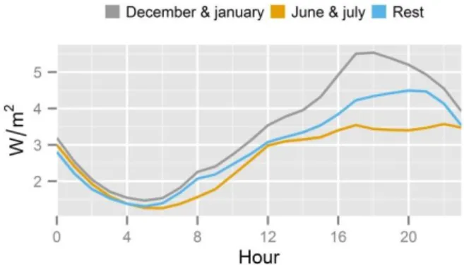
Fig. 4 shows measured average household electricity demand in 2011 and 2012 for 192 randomly selected apartments. 217

8

This represent about 44% of the total stock of 438 apartments in the Lagersberg district. All household electricity 218

consumption is assumed to end up as heat gains, thus decreasing the building’s heat demand. Impact on heat demand is 219

modelled as a 25% annual decrease of household electricity consumption, distributed accordingly to the schedule of 220

Fig. 4. Therefore the impact will be higher at afternoons than during nights and higher in the winter than during 221

summer. 222

223

Fig. 4. Measured diurnal variation of household electricity consumption for 192 households, grouped by time of year.

224

2.2.5 Domestic hot water

225

Measures to reduce domestic hot water (DHW) consumption include use of water-efficient showerheads and taps and 226

insulation of DHW recirculation piping. Another such measure is individual metering and charging of DHW instead of 227

including it in the rent or tenant fee. DHW savings are simulated as a uniform decrease over the year, appearing as a 228

straight line when average daily DHW saving is plotted against time as diurnal variations are evened out. 229

2.2.6 Exhaust air heat pump

230

The annual electricity-to-heat factor (often referred to as seasonal performance factor) for an EAHP depends on factors 231

such as working mode (space heating or domestic hot water) and connection scheme. The ESBO plant module in IDA 232

ICE is used to model the EAHP, see [25,26] for more details. The EAHP is modelled to deliver heat for both space 233

heating and domestic hot water, dimensioned to take 1/3 of the exhaust air flow and connected to a 1 m3 stratification

234

tank. The EAHP impact on the DH return temperature is not accounted for in this study. 235

2.2.7 Thermal solar

236

The thermal solar system is modelled with the ESBO [25] module in IDA ICE to deliver heat for both space heating and 237

domestic hot water, and is dimensioned after domestic hot water consumption during the summer season. 238

2.3

239

Heat demand profiles for the studied ECMs are acquired by calculating the daily difference between the district heating 240

demand of the baseline model and the model including the ECM, resulting in vectors of 365 daily mean values which 241

are scaled to the annual sum of 1 MWh. Each of these 365 values has a corresponding set of weather variables in the 242

TMY weather data and the TMY heat load of the DHS. Daily average values are selected based on the assumption that 243

the dynamic effect of the buildings’ heat storage capacity can be neglected. 244

2.4

245

Weather normalised heat load of the DHS is derived from regression coefficients of weather and heat load data from 246

2012-2014 which are used with TMY weather data to calculate the weather normalised heat load. Multiple linear 247

regression of the form 𝑌 = 𝛽0+ 𝛽1∗ 𝑥1+ ⋯ + 𝛽𝑝∗ 𝑋𝑝+ 𝜀 is used, where 𝑌 denotes the response variable (heat

9

load), 𝛽₀ denotes the intercept, 𝑥₁, … , 𝑥_𝑝 are explanatory variables with coefficients 𝛽₁, … , 𝛽_𝑝 and 𝜀 represents the

249

unexplained part. The regression coefficients 𝛽 are calculated using the lm function in the R statistical programming 250

language. 251

Fig. 5 illustrates how historical heat loads and weather data (a and b) are segmented by the use of heating degree days 252

(c). Through linear regression (d) and segmentation by TMY weather data (e and f) the regression coefficients are 253

determined (g). Finally, the weather normalised heat load can be calculated (h). Heating degree days (HDD) is used to 254

find change points for the segmentation and is calculated as the mean difference between the assumed balance 255

temperature of 17°C and the hourly outdoor temperature for each hour per day: 𝐻𝐷𝐷 = ∑24ℎ=1(𝑇𝑏− 𝑇𝑜)+, where the +

256

symbol indicates that negative values are set to zero. In the final model the dataset is segmented into four sets: summer, 257

heating, transition and very cold segments. Days with HDD lower than 35°Ch are categorised as summer, days with 35 258

- 120°Ch are categorised as transition period, 120 - 530°Ch as heating and over 530°Ch as very cold. These boundaries 259

are selected manually by minimising the RMSE. 260

261

Fig. 5. The heat load weather normalisation process.

262

Five explanatory variables are included in the final model: outdoor temperature, global solar radiation, ground 263

temperature, temperature change and wind speed. The purpose is to obtain a good prediction, not to interpret the 264

included explanatory variables. As shown in Table 2, all included variables contribute to a better prediction, even 265

though outdoor temperature is by far the most important variable. The root mean square error (RMSE) is used as a 266

metric of prediction power and is calculated with cross-validation by splitting the data into two datasets by placing the 267

first 15 days of each month in one set and the remaining days in the second set. Heat load is then predicted for one of 268

Table 2. Root mean square error (RMSE) and normalised RMSE of predicted district heating production on daily basis. Each column show the prediction power of the model if excluding a variable, ‘none’ denotes the full model with no excluded variables

Excluded variable none Wind speed Temperature change Ground temperature Global solar irradiation Outdoor temperature RMSE [MW] 4.9 5.3 5.3 5.4 6.7 16.2 Normalised RMSE [%] 2.2% 2.4% 2.4% 2.4% 3.0% 7.2%

Fig. 6. Correlation of DHS model residuals and outdoor temperature when segmenting into two, three or four seasons when all explanatory variables are included into the model. Solid line: local linear regression, dashed line: linear regression.

10

the datasets and validated against the other dataset, and vice versa. Ground temperature is calculated as the average of 269

the mean annual outdoor temperature and the mean outdoor temperature of the last 30 days. Temperature change is 270

calculated as the difference between the mean temperature of the current date and the day before. Fig. 6 shows the 271

impact of segmentation: adding the transition period (three segments) improves the model substantially (visualised by 272

the much more uniformed residuals), as the change point between heating and summer season is not as sharp for a 273

whole DHS as for a single building. Adding the cold seasons (four segments) has almost no impact on the RMSE but as 274

the accuracy increases at the peak load production (which has a strong influence on environmental and economic 275

assessments) the fourth segments are still added. 276

2.5

277

The applied method builds on the method presented in [27]. Production cost of district heating is described by the cost 278 function 279 𝒚 = ∑ (𝒙𝒊× 𝑪𝒐𝒔𝒕𝒊+ 𝒙𝒊× 𝜶𝒊× (𝑪𝒐𝒔𝒕𝒊− 𝑰𝒏𝒄𝒐𝒎𝒆𝒊)) 𝒏 𝒊 (1)

where 𝑦 is the total cost, 𝑥𝑖 is the amount of district heating produced for unit 𝑖, 𝐶𝑜𝑠𝑡𝑖 is the production cost per unit

280

thermal heat (includes fuel cost, environmental taxes and plant efficiency), 𝛼𝑖 is the ratio of electricity produced per unit

281

produced heat and 𝐼𝑛𝑐𝑜𝑚𝑒𝑖 includes revenue from selling electricity.

282

283

Fig. 7. Heat load duration of the Eskilstuna DHS model. Daily mean heat and electricity production for a TMY. Flue gas condensing

284

is included in CHP and biomass HO plants.

285 286

The cost function (1) is minimised by using the constrained nonlinear multivariable function finder fmincon, available 287

in the Matlab Optimization Toolbox. Constrains are set as ∑𝑛𝑖𝑥𝑖= total heat load; 𝒙 ∈ [0, 𝒖𝒃], where 𝒖𝒃 is the upper

288

bounds vector (maximum capacity for each unit); 𝑥𝑗≤ 𝛼𝑖 × 𝑥𝑖 where 𝑖 is a CHP plant and 𝑗 is the turbine bypass of

289

that CHP plant; 𝑥𝑗≤ 𝑢𝑏𝑗/𝑢𝑏𝑖, where 𝑖 is a CHP plant and 𝑗 is the flue gas condenser of that CHP plant. Table 3

290

presents the parameters used. The heat storage tank is not included in the optimisation model under the assumption that 291

it will mostly level out diurnal variation, hence daily average values are used. Heat losses in the district heating 292

pipelines (about 12% on yearly basis) are omitted. Depending on marginal heat production cost and the electricity 293

selling price the CHP-plant can produce both heat and electricity or bypass the turbine (thus producing heat only). 294

Based on temperature and electricity price data from 2006 to 2014 there have on average been 21 days per year with 295

average temperatures under the -5°C, where peak heat need to be produced by either by oil boilers or by bypassing the 296

turbine. For 13% of these days electricity prices were high enough so it would be profitable to produce heat via oil 297

boilers rather than bypassing the turbine. This has been included in the model. Fig. 7 shows the heat and electricity 298

11

production for a typical weather year. 299

Table 3. Parameters used in the Eskilstuna DHS model

300 Unit CHP FGC Bypass turbine Biomass HO* Oil HO Production cost (SEK/MWh) 250 0 250 220 750 Capacity (MW) 72 24 38 70 No limit Efficiency 0.9 1 1 1.02 0.8 α-value 0.53 - -1 - - * include FGC 301 302

To validate the model, it is run with electricity and weather data of 2012 and compared to the real production mix of 303

that year. As shown in Table 4 the modelled and the actual production match reasonable well. The model generates 304

higher production values for the CHP which to a large part is explained by that the model does not consider downtime 305

which according to the plant manager occurred more frequently during 2012 than normally. This also partly explains 306

the higher electricity production value for the model. Electricity production is also affected by that the model does not 307

consider part load conditions which gives lower α-values compared to the used nominal values. 308

Table 4. The measured and modelled production mix of 2012

309 Unit Measured [GWh/y] Modelled [GWh/y] CHP incl. FGC 548 577 Bypass turbine 12* 15 Biomass HO incl. FGC 204 193 Oil HO 40 21

Total heat production 804 807 Electricity production 195 215

*Estimated from the difference between real and possible electricity production

310 311

2.6

312

The typical meteorological year (TMY) weather data used for Eskilstuna, also known as test reference year, were 313

acquired from [28] and are described in [29]. A TMY consists of real observations but with each month originating 314

from a different calendar year. These are selected by comparing the frequency distributions of daily climatic variables 315

during a single month of a candidate year with the corresponding distributions for the same calendar month but based 316

on data from a 30 year period. Historical weather data were acquired from the Swedish Meteorological and 317

Hydrological Institute (SMHI) metrological weather station in Eskilstuna; modelled solar irradiation data were obtained 318

from the SMHI STRÅNG project [30]. The data acquisition and conversion of weather data is processed through this 319

tool [31]. 320

2.7

321

Electricity CO2 and PE (primary energy) factors are selected that roughly correspond to first and third quartiles of in

322

Sweden commonly used factors, defined as low and high in Table 5. The low values for electricity correspond to yearly 323

average of the historical electricity production mix in the Nordic countries [20,21]. The high values correspond to an 324

expected near future with marginal electricity production covered by natural gas combine power plants [10,20]. This 325

approach gives the possibility to linearly interpolate or extrapolate the results to meet the perspective of the readers’ 326

choice. See [23] for more discussion regarding emission factors for Nordic electricity production. For biomass fuels a 327

12

fossil CO2 emission factor of 16 kg/MWh is used [21,22], which accounts for emissions from handling and

328

transportation. The low PE factor for biomass corresponds to case when biomass is considered as a residual product 329

without any PE value [21], fuel handling and transportation is still accounted for. The high PE factor corresponds to the 330

case when the biomass is considered to have a full PE value [21]. The oil is composed of a 50% mixture of bio-based 331

and fossil-based why lower values compared to traditional fossil-based oil are shown in the table. 332

Table 5. Used fossil CO2 and PE factors

333

Energy carrier PE factor (MWh/MWh) CO2 (kg/MWh)

Low High Low High

Electricity 1.5 2.5 100 400

Biomass 0.1 1.1 16 16

Oil (bio and fossil) 0.6 1.1 160 160

3

334

3.1

335

The annual electricity-to-heat factors in Table 6 describe the connection between annual heat and electricity demands, 336

e.g. decreasing the ’electricity consumption’ by 1 kWh/y would lead to a 0.69 kWh/y increase in heat demand. These 337

values are obtained by simulation and are valid for buildings and weather conditions similar to those studied in this 338

paper. At higher outdoor temperatures when no space heating is needed, changes in electricity consumption will not 339

have any impact heat demand. Therefore annual electricity-to-heat factors will be less than 1 for electricity saving 340

measures. The factor depends upon the balancing temperature of the building, the local climate, the extent that heat 341

dissipation from equipment displaces heat demand and at what time the electricity is consumed. 342

Table 6. Annual electricity-to-heat factors

343

ECM Electricity consumption EAHP HRV

Factor 0.69 3.2 10

344

The results for electricity consumption and ‘HRV’ are quite straightforward. But for the ‘EAHP’ the result can vary 345

substantially depending on connection scheme, working mode, etc. The annual electricity-to-heat factor agrees well 346

with results in paper [32]. The ‘EAHP’ connection scheme can also affect the return temperature, which will affect the 347

DHS, which is not accounted for in this study. 348

3.2

349

Fig. 8 shows heat demand profiles of ECMs. The heat demand of the baseline model is added for 350

comparison. All values are scaled to 1 MWh/y, for comparability reasons. The y-axis shows the change in 351

heat demand as daily mean power [kW]. In order to obtain a clearer view smoothened trend lines are shown 352

in Fig. 8, not actual data points. The grey shaded area shows the local confidence interval at a standard error 353

(SE) of 95% and is a measure of local variation. Subfigure (a) shows the heat demand duration curve (daily 354

values on the x-axis are arranged in ascending order according to the heat demand of the baseline model). 355

Subfigures (b and c) show the correlation to outdoor temperature and solar radiation and indicate under 356

which weather conditions in the ECMs will have an impact. Subfigures (a and b) appears quite similar as 357

outdoor temperature is the factor having the strongest impact on energy consumption. However the duration 358

13

curve also provides information about the number of certain level of savings is obtained (thus the area in-359

between the lines, zero and the duration equals energy). For example, the curve of ‘HRV’ suggest it perform 360

poorly at low temperatures compared to ‘building envelope’ (see Fig. 8b), but it is also clear that the 361

duration of this occurrence is limited in time (see Fig. 8a). Thereby these hours do not affect energy 362

consumption considerable, but still affect the peak load. Obviously ‘thermal solar’ correlates strongly to the 363

level of solar radiation, it also correlates to outdoor temperature as outdoor temperature is a good indicator 364

of time of the year and thereby the probability of solar radiation. ‘Operational optimisation’ mostly 365

contribute at mild weather when there are still need for space heating and more overheating issues due to 366

solar gains and fast outdoor temperature changes. The duration curve illustrates that ‘thermal solar’ does not 367

contribute at all to reduce peak loads, also ‘operational optimisation’ contribute poorly to reduce peaks. The 368

‘ERV’ (not included in the figure) is essentially identical to the profile of the ‘building envelope’. 369

370

Fig. 8. Heat demand profiles of the baseline building model and the ECMs, scaled to the annual sum of 1 MWh heat. Lines are

371

smoothed by local linear regression and grey shaded areas show local confidence interval at standard error of 95%.

372 373

3.3

374

Fig. 9b shows the resulting marginal impact of ECMs on the DHS heat producing units and how the electricity balance 375

(production and consumption) is affected. Impact on PE and CO2, accounting for the impact on the electricity balance,

376

is shown in Fig. 9c. All values are scaled to 1 MWh of change in annual heat demand (1MWh increase for ‘household 377

electricity’ and 1MWh decrease for the other ECMs), this makes it possible to compare the impact from studied ECMs. 378

Resulting values can also be used as factors to estimate the absolute impact from an ECM or a package of ECMs, which 379

the developed interactive tool at https://reesbe.shinyapps.io/eskilstuna is an example of. 380

There is a strong connection between the shape of the heat demand profiles of the ECMs and the impact on the DHS. 381

The heat load strongly correlates to the outdoor temperature, thereby measures such as ‘building envelope’ and ‘HRV’ 382

that reduce heat demand at low outdoor temperatures have more favourable impacts on the DHS. However, the most 383

important parameters for the environmental assessment are to which degree the electricity consumption is affected (i.e. 384

electricity-to-heat factors in Table 6) and which PE and CO2 factors that are assigned to the electricity and biomass

385

fuels. 386

14

Improving the building envelope has a positive impact on the DHS independent of the environmental emissions 387

perspective. This is due to the reduced need for bypassing the DHS turbine in cold weather resulting in an increase in 388

electricity production which roughly equals the reduction in electricity cogeneration in milder weather. Reducing 389

household electricity consumption would have the most favourable environmental impact, partly because it would allow 390

for more electricity cogeneration at the CHP. 391

392

Fig. 9. Marginal impact of ECMs, scaled to 1 MWh of change in annual heat demand. Positive values indicate a decrease/saving,

393

negative values indicate an increase, (a) miniatures of Fig. 8a, (b) wider bars show impact on heat producing units; the two narrow

394

bars show the impact on the electricity cogeneration and consumption and (c) marginal impact on PE and CO2

395 396

4

397

The Eskilstuna DHS has an exceptionally high share of renewable fuels and electricity cogeneration, and hence a low 398

fossil CO2 emission rate. The Eskilstuna case study is therefore not easily generalizable to other current DHSs.

399

Nevertheless, it is an interesting case as it highlights the forthcoming problem of diminishing environmental benefits 400

from ECMs. In future, more Nordic DHSs are likely to have similar characteristics as heat demand decreases and DH 401

production becomes “greener” and more efficient. At some point, benefits from decreasing heat demand due to ECMs 402

in DH connected buildings will diminish. In Central & Western Europe, China and other countries where DH have 403

small to medium market shares, this is less of an issue as heat demand savings can be met by expanding the DH 404

15

networks. 405

Improving buildings envelope and installing heat/energy recovery ventilation level out the DHS heat load duration 406

curve, which will allow reduced future investment in peak load plants and higher utilisation rate of future base load 407

plants. 408

The presented weather normalisation method and heat demand profiles could be used for example a) to predict how 409

future DH heat load would look if an assumed/known package of ECMs were applied to a building stock; b) to design 410

policies and price models to incentivise a desired future DH heat load; c) to take into account expected future climate 411

warming by using climate files similar to those derived for Finland [33]. In paper [34] Finnish heating demand is 412

predicted to decrease by about 3% per decade due to global warming. 413

The energy recovery ventilation (ERV) heat demand profile appears similar to the profile of the ‘building envelope’ in 414

Fig. 8. These measures provide a greater saving in cold weather than heat recovery ventilation (HRV). In years with 415

extreme cold weather the differences between ERV and HRV would be larger, and therefore simulating HRV under 416

TMY weather conditions may lead to misleadingly favourable results. ERV is usually not installed in residential 417

buildings because of problems with moisture accumulation and odour recovery to the supply air stream. However, from 418

an energy system point of view ERV appears to be a better option than HRV. 419

Table 1 gives a rough picture of heat savings potentials for typical Swedish multifamily buildings that are due to 420

renovation. Recovering heat from the ventilation system and improving the building envelope have the largest potential, 421

while other studied ECMs show less potential. But feasibility of ECMs is also dependent on the investment cost. For 422

example operational optimisation can be relative cost-effective and can thereby still be expected to give significant 423

contribution to heat savings when looking on a package of ECMs for a whole stock of buildings. 424

5

425

The environmental impact of each ECM in terms of primary energy (PE) and CO2 emissions is strongly influenced by

426

the choice of assessment perspective. Reducing electricity consumption and improving the building envelopes are the 427

only ECMs that are favourable regardless of the choice of assessment factors. If biomass fuels are not considered a 428

residual and are assigned a PE factor of 1.1 then all studied ECMs do increase primary energy efficiency. 429

Heat demand profiles and annual electricity-to-heat factors vary for ECMs. It is not only the amount of energy that can 430

be saved but also at what time of the year the energy can be saved that matters. Saving heat by increasing electricity 431

consumption does not improve primary energy efficiency or mitigate global warming. ECMs with energy system-432

favourable heat demand profiles and high annual electricity-to-heat factors should be prioritised. 433

The weather normalisation method presented in Section 2.4 proves useful for getting the heat load of the DHS model

434

and heat demand savings of the building model to work under the same (and typical) weather conditions. The freely 435

available modelled solar hourly irradiation database STRÅNG from SMHI increases the prediction power. 436

Acknowledgements

437

The work has been carried out under the auspices of the industrial post-graduate school Reesbe. Financers are 438

Eskilstuna Kommunfastigheter, Eskilstuna Energy & Environment and the Knowledge Foundation (KK-stiftelsen). 439

16

References

440

[1] European Parliament and the Council of the European Union. Energy performance of buildings directive.

441

Directive 2010/31/EU; 2010. 442

[2] Jennings M, Fisk D, Shah N. Modelling and optimization of retrofitting residential energy systems at the urban

443

scale. Energy 2014;64:220–33. doi:10.1016/j.energy.2013.10.076. 444

[3] Gustavsson L. District heating systems and energy conservation—part I. Energy 1994;19:81–91.

445

doi:10.1016/0360-5442(94)90107-4. 446

[4] Gustavsson L. District heating systems and energy conservation—Part II. Energy 1994;19:93–102.

447

doi:10.1016/0360-5442(94)90108-2. 448

[5] Frederiksen S, Werner S. District Heating and Cooling. First. Lund: Studentliteratur; 2013.

449

[6] Connolly D, Mathiesen BV, Østergaard PA, Möller B, Nielsen S, Lund H, et al. HEAT ROADMAP EUROPE

450

2050. Aalborg: 2013. 451

[7] Difs K, Bennstam M, Trygg L, Nordenstam L. Energy conservation measures in buildings heated by district

452

heating – A local energy system perspective. Energy 2010;35:3194–203. doi:10.1016/j.energy.2010.04.001. 453

[8] Gustavsson L, Dodoo A, Truong NL, Danielski I. Primary energy implications of end-use energy efficiency

454

measures in district heated buildings. Energy Build 2011;43:38–48. doi:10.1016/j.enbuild.2010.07.029. 455

[9] Truong N Le, Dodoo A, Gustavsson L. Effects of heat and electricity saving measures in district-heated

456

multistory residential buildings. Appl Energy 2014;118:57–67. doi:10.1016/j.apenergy.2013.12.009. 457

[10] Åberg M. Investigating the impact of heat demand reductions on Swedish district heating production using a set

458

of typical system models. Appl Energy 2014;118:246–57. doi:10.1016/j.apenergy.2013.11.077. 459

[11] Harrestrup M, Svendsen S. Changes in heat load profile of typical Danish multi-storey buildings when

energy-460

renovated and supplied with low-temperature district heating. Int J Sustain Energy 2013;34:232–47. 461

doi:10.1080/14786451.2013.848863. 462

[12] Harrestrup M, Svendsen S. Heat planning for fossil-fuel-free district heating areas with extensive end-use heat

463

savings: A case study of the Copenhagen district heating area in Denmark. Energy Policy 2014;68:294–305. 464

doi:10.1016/j.enpol.2014.01.031. 465

[13] Klobut K, Heikkinen J, Shemeikka J, Laitinen A, Rämä M, Sipilä K. Huippuenergiatehokkaan asuintalon

466

kaukolämpöratkaisut [District heating solution for very-low-energy residential building]. 2009. 467

[14] Swedish District Heating Association. Supply energy mix 1980-2012 (Tillförd energi utveckling 1980-2012)

468

n.d. http://www.svenskfjarrvarme.se/Statistik--Pris/Fjarrvarme/Energitillforsel/Tillford-energi-utveckling-1980-469

2012 (accessed August 10, 2015). 470

[15] Statistics Sweden (SCB). Annual energy statistics (Årlig energistatistik - Bränsleförbrukning för elproduktion i

471

Sverige efter produktionsslag och bränsletyp. År 1990 - 2013) 2014. http://www.scb.se/en0105 (accessed 472

August 10, 2015). 473

[16] Heller AJ. Heat-load modelling for large systems. Appl Energy 2002;72:371–87.

doi:10.1016/S0306-474

2619(02)00020-X. 475

[17] Aronsson S. Fjärrvärmekunders värme- och effektbehov : analys baserad på mätresultat från femtio byggnader

476

= [Heat load of buildings supplied by district heating] : [an analysis based on measurements in 50 buildings] / 477

av Stefan Aronsson. Göteborg : Chalmers tekniska högsk., 1996 ; (Göteborg : Teknologtr., Chalmers); 1996. 478

17

[18] Andersson S, Sjögren J-U, Östin R, Olofsson T. Building performance based on measured data n.d.

479

[19] Vesterberg J, Andersson S, Olofsson T. Robustness of a regression approach, aimed for calibration of whole

480

building energy simulation tools. Energy Build 2014;81:430–4. doi:10.1016/j.enbuild.2014.06.035. 481

[20] Sjödin J, Grönkvist S. Emissions accounting for use and supply of electricity in the Nordic market. Energy

482

Policy 2004;32:1555–64. doi:10.1016/S0301-4215(03)00129-0. 483

[21] Gode J, Martinsson F, Hagberg L, Palm D. Miljöfaktaboken 2011 - Estimated emission factors for fuels,

484

electricity, heat and transport in Sweden (Uppskattade emissionsfaktorer för bränslen, el, värme och 485

transporter). Stockholm: Värmeforsk; 2011. 486

[22] Swedish District Heating Association - Environmental assets 2012 (Svensk Fjärrvärme - Miljövärden 2012)

487

2012. http://www.svenskfjarrvarme.se/Fjarrvarme/Miljovardering-av-fjarrvarme/Miljovarden-2012/ (accessed 488

December 15, 2013). 489

[23] Dotzauer E. Greenhouse gas emissions from power generation and consumption in a nordic perspective. Energy

490

Policy 2010;38:701–4. doi:10.1016/j.enpol.2009.10.066. 491

[24] Levin P, Karlsson C. Rekorderlig Renovering – Demonstrationsprojekt för energieffektivisering i befintliga

492

flerbostadshus – Slutrapport för Lagersbergs renoveringsetapp1 – Kommunfastigheter i Eskilstuna. Stockholm: 493

2015. 494

[25] Equa. IDA Early Stage Building Optimization (ESBO). Version 109 2013.

495

http://www.equaonline.com/esbo/IDAESBOUserguide.pdf (accessed April 27, 2015). 496

[26] Maivel M, Kurnitski J. Heating system return temperature effect on heat pump performance. Energy Build

497

2015;94:71–9. doi:10.1016/j.enbuild.2015.02.048. 498

[27] Åberg M, Widén J. Development, validation and application of a fixed district heating model structure that

499

requires small amounts of input data. Energy Convers Manag 2013;75:74–85.

500

doi:10.1016/j.enconman.2013.05.032. 501

[28] Sveby & SMHI. Klimatfiler 81-10 SvebySMHI 2015.

http://www.sveby.org/wp-502

content/uploads/2011/09/Klimatfiler-81-10-Sveby-SMHI.rar (accessed March 6, 2015). 503

[29] Levin P, Clarholm A, Andersson C. Nya klimatfiler för energiberäkningar. Stockholm: 2015.

504

[30] SMHI. STRÅNG - a mesoscale model for solar radiation n.d. http://strang.smhi.se (accessed August 5, 2015).

505

[31] Lundström L. RTWC n.d. https://sites.google.com/site/weatherconverter (accessed April 27, 2015).

506

[32] Mikola A, Kõiv T-A. The Efficiency Analysis of the Exhaust Air Heat Pump System. En-Gineering

507

2014;6:1037–45. doi:10.4236/eng.2014.613093. 508

[33] Jylhä K, Kalamees T, Tietäväinen H, Ruosteenoja K, Jokisalo J, Hyvönen R, et al. Rakennusten

509

energialaskennan testivuosi 2012 ja arviot ilmastonmuutoksen vaikutuksista (Test reference year 2012 for 510

building energy demand and impacts of climate change). Helsinki: 2012. 511

[34] Jylhä K, Jokisalo J, Ruosteenoja K, Pilli-Sihvola K, Kalamees T, Seitola T, et al. Energy demand for the heating

512

and cooling of residential houses in Finland in a changing climate. Energy Build 2015. 513

doi:10.1016/j.enbuild.2015.04.001. 514