Weak Boundary and Interface Procedures for Wave and Flow Problems

(1)

(2)

(3)

(4)

(5)

List of Papers

This thesis is based on the following papers, which are referred to in the text by their Roman numerals.

I Abbas Q., Nordström J. (2010) Weak versus strong no-slip boundary conditions for the Navier-Stokes equations. Engineering Applications of Computational Fluid Mechanics, 4(1): 29–38.

II Abbas Q., Nordström J. (2011) A weak boundary procedure for high order finite difference approximations of hyperbolic problems. Uppsala University Technical Report No. 2011-019. Submitted.

III Abbas Q., van der Weide E., Nordström, J. (2009) Accurate and stable calculations involving shocks using a new hybrid scheme. AIAA Paper No. 2009-3985.

IV Eriksson S., Abbas Q., Nordström J. (2011) A stable and conserva-tive method for locally adapting the design order of finite difference schemes. Journal of Computational Physics, 230(11):4216–4231. V Abbas Q., van der Weide E., Nordström, J. (2010) Energy stability of

the MUSCL scheme. In Numerical Mathematics and Advanced Appli-cations 2009, pages 61–68.

VI Law, C., Abbas, Q., Nordström, J., Skews, B.W. (2010) The effect of Reynolds number in high order accurate calculations with shock diffrac-tion. In Proceedings of 7th South African Conference on Computational and Applied Mechanics, pages 416–423.

(6)

(7)

Related Work

Although not explicitly discussed in the comprehensive summary, the follow-ing papers are related to the contents of this thesis.

• Pettersson, P., Abbas, Q., Iaccarino, G., Nordström, J. (2010) Efficiency of shock capturing schemes for Burgers’ equation with boundary uncertainty. In Numerical Mathematics and Advanced Applications 2009, pages 737– 745.

• Khan M., Abbas Q. and Duru K. (2010) Magnetohydrodynamic flow of a Sisko fluid in annular pipe: A numerical study. International Journal for Numerical Methods in Fluids, 62:1169–1180.

(8)

(9)

1. Introduction

Partial differential equations (PDEs) arise in the modeling of numerous phe-nomena in science and engineering such as fluid flow, heat transfer, solid me-chanics and biological process. Roughly speaking, a PDE is an equation that involves unknown functions of several variables and their derivatives. These equations often fall into three categories, hyperbolic, parabolic, and elliptic equations. Mixtures are also common, for example, the advection–diffusion equation involves important aspects of both hyperbolic and parabolic prob-lems [1]. A PDE with initial and boundary conditions is often refereed to as an initial boundary value problem (IBVP).

This thesis addresses the numerical solution of IBVPs. In particular, we aim to solve time-dependent wave propagation and flow problems. A recipe for solving such problems typically requires proper treatment of (i) advection and diffusion terms, (ii) artificial dissipation terms, and (iii) boundary condi-tions. There is a variety of different solution methods for time-dependent par-tial differenpar-tial equations including for example finite difference, finite vol-ume, finite element and spectral methods. They all have different strengths and drawbacks. Our contribution in this thesis includes the treatment of all the three topics mentioned above for the finite difference method.

1.1 Short summary of previous work

High order finite difference methods are suitable to accurately compute the fine structures of time dependent problems, but the implementation of bound-ary conditions in a stable manner is non-trivial [2, 3, 4, 5].

Summation-By-Parts (SBP) operators for first derivative approximations were derived in [6] by Strand as an extension of the work by Kreiss and Scherer [7, 8]. Stability for these SBP schemes was proved for periodic prob-lems by using the energy method. SBP operators of different orders of accu-racy approximating d/dx and d2/dx2have also been constructed in [9, 10].

Carpenter et al. [4, 11] introduced a new way to implement boundary con-ditions for finite difference methods with the Simultaneous Approximation Term (SAT) method. The SAT method (weak imposition of boundary con-dition or penalty technique) imposes boundary concon-ditions such that the SBP property is preserved and leads to an energy estimate.

(12)

Another way to implement boundary conditions was developed by Olsson [12, 13], where the so called projection method was used. An analysis of the different ways of implementing boundary conditions using projection, injec-tion and SAT technique was done by Mattsson in [14]. The SAT technique was found to be superior to the other implementations.

In a series of articles by Nordström et al. [9, 15, 16], this technique was developed for advection-diffusion problems and the Navier-Stokes equations including extensions to stable and conservative interface conditions. In this thesis, we have further investigated and extended the SBP-SAT technique.

1.2 Continuous and discrete energy estimates

Consider the one-dimensional right going (a > 0) advection problem

ut+ aux= 0, 0≤ x ≤ 1, t > 0, (1.1)

with a boundary condition u(0,t) = g0(t) for well-posedness [17, 18]. By

mul-tiplying (1.1) with u and integrating over the domain yields the following en-ergy rate

d dt∥u∥

2_{= au(0,t)}2_{− au(1,t)}2_, _(1.2)

where ∥u∥2 =∫₀1u2dx. By inserting u(0,t) = g0(t), an energy estimate

fol-lows.

Let the approximate solution at grid point xi (= x0+ i∆x) be denoted by

ui, and the discrete solution vector uT = [u0, u1, . . . , uN]. A semi-discrete

fi-nite difference approximation of (1.1) using an SBP operator with the SAT treatment for the boundary conditions can be written as

ut+ aP−1Qu = P−1α00(u0− g0) e0. (1.3)

Here the difference operator P−1Q approximates d/dx. P is a diagonal and positive definite matrix, Q + QT = B = diag (−1,0,...,0,1),α00is called the

penalty coefficient and e0= [1, 0, . . . , 0]T. By multiplying (1.3) by uTP and

adding its transpose gives d dt∥u∥

2

P= (a + 2α00) u20− 2α00u0g0− au2N, (1.4)

where∥u∥2_P= uTPu. Forα00≤ −(a/2), we have a bounded energy. Without

boundary conditions (α00 = 0), the rate (1.4) mimics (1.2) perfectly. More

elaborate discussions regarding this technique can be found in [6, 9, 11, 14, 19]. In Section 2.1, we have further discussed this technique.

(13)

There is no general procedure to obtain stability when using strong bound-ary conditions and high order difference schemes. In fact, it has been shown that strong boundary conditions may ruin the stability [20, 21] even for low order operators.

1.3 Weak boundary conditions at multiple grid points

The SAT technique is normally applied only at one grid point. However, it is possible to impose the boundary conditions at multiple grid points. This has many advantages, and gives the designer of the scheme flexibility and options. This technique can be used where the solution is known, for example at far-field boundaries.

To illustrate the procedure, we add additional penalty terms in (1.3) at two new grid points x1and x2, close to the boundary x = 0 as

ut+ aP−1Qu = P−1{α00(u0− g0) e0+α01(u1− g1) e0

+α10(u0− g0) e1+α11(u1− g1) e1+α12(u2− g2) e1

+α21(u1− g1) e2+α22(u2− g2) e2},

(1.5)

where e1= [0, 1, . . . , 0]T and e2 = [0, 0, 1, . . . , 0]T. αi j with i, j ={0,1,2},

are the penalty coefficients and gi with i ={0,1,2}, are the boundary data.

Equation (1.5) is as accurate as the original scheme (1.3) as long as g1(∆x,t)

and g2(2∆x,t) are known. Next we apply the energy method to (1.5) with

gi= 0. The result corresponding to (1.4) with g0= 0 becomes

d dt∥u∥ 2 P=    u0 u1 u2    T   a + 2α00 α01+α10 0 α01+α10 2α11 α12+α21 0 α12+α21 2α22    | {z } R    u0 u1 u2    − au2 N.

For stability, we need to chooseαi j, such that the matrix R is negative

semi-definite. The most obvious choice would be Rii≤ 0 and Ri j= 0 for i̸= j.

In Paper II, initial work has been done where this technique has been found to be very useful for obtaining higher accuracy, improved convergence rate to steady-state, and non-reflecting boundary conditions. More details are given in Section 2.2.

1.4 Artificial dissipation operators

Since an SBP operator is essentially a centered difference scheme, added ar-tificial dissipation is required for shock calculations in order to reduce

(14)

non-physical numerical oscillations [22, 23, 24]. A semi-discrete approximation of (1.1) including an artificial dissipation operator DI2pcan be written,

ut+ aP−1Qu = DI2pu +α00P−1(u0− g0)e0. (1.6)

In [22], a higher order accurate artificial dissipation operator DI2pis given by

DI2p=−P−1DTPBPDP, (1.7)

where Dp is a consistent approximation of hp(dp/dxp). Bp is a symmetric

positive semi-definite matrix. Inserting (1.7) into (1.6) and applying the energy method yields d dt∥u∥ 2 P+ 2 Dpu 2 Bp= (a + 2α00) u 2 0− 2α00u0g0− au2N, (1.8) where Dpu 2_B p = (Dpu) T_B

p(Dpu). By comparing with (1.4), the artificial

dissipation operator DI2p introduces an extra term Dpu 2

Bp in (1.8) which

dissipates energy.

In Papers III–VI, we have used artificial dissipation terms of the form (1.7), for problems involving discontinuities and shocks. Further details on its use are given in Sections 2.3–2.6.

1.5 Hybrid schemes

It is well known that higher order central schemes exhibit oscillations around shocks, but are very efficient for smooth solutions [25]. To resolve shocks and avoid oscillations, the numerical scheme must be first order in the vicinity of the shock. At the same time the scheme must be higher order in smooth regions to resolve fine structures of the solution. In flow fields where both fea-tures exist, both the shock capturing capability and the higher order accuracy are required.

Many people have worked on blends of different numerical methods to get a scheme with appropriate features [26, 27, 28, 29, 30]. Although some of the previous attempts have been successful, most of the schemes have been devel-oped for Cauchy problems or problems with periodic boundary conditions.

In Paper III, we construct a hybrid scheme in such a way that it is a second order accurate MUSCL (Monotone Upstream-centered Schemes for Conser-vation Laws) scheme in the shock region and a high order central scheme in the smooth regions away from the shock. The scheme is written in the framework of SBP operators and artificial dissipation terms, so that an energy estimate and linear stability can be guaranteed.

A similar approach was used in Paper IV. A stable procedure for locally changing order of the method was developed. The procedure is useful when

(15)

the order of a numerical scheme has to be lowered in a small region (at a discontinuity or shock). It was combined with the shock capturing MUSCL scheme. Both scalar and first order systems of equations in one dimension were considered.

1.6 Computation of shocks and boundary layers

In Paper VI, we combine some of the techniques developed in this thesis to a complex flow case including both shocks and boundary layers. The flow be-hind shocks diffracting around convex walls was investigated in [31], using a combination of experiments and computational techniques. The second order finite volume solver was unable to resolve the fine features in the complicated flow field.

Our high order finite difference solver based on the SBP-SAT technique was used to study the shock diffraction problem mentioned above. In this calcu-lation, we used the artificial dissipation technique to get first order one-sided schemes in the vicinity of shocks. This provided numerical stability close to the shock while retaining higher order accuracy everywhere else in the flow field. We have further discussed this calculation in Section 2.6.

(16)

(17)

2. Summary of Papers

2.1 Paper I

In [32], a high order accurate solid wall boundary procedure for the com-pressible Navier-Stokes equations which is stable due to the SAT technique and SBP operators was presented. In Paper I, we extend the analysis of no-slip wall boundary conditions and focus on the accuracy aspects, especially for coarse realistic meshes.

As a model problem, we considered the following advection-diffusion prob-lem in one space dimension,

ut+ aux=εuxx, 0≤ x ≤ 1, t ≥ 0,

u(0,t) = g0(t),

u(1,t) = gN(t),

u(x, 0) = f (x).

(2.1)

In (2.1) a,ε > 0 and ε << a. The semi-discrete form of (2.1) using SBP op-erators and SAT technique is given by

vt+ aP−1Qv =εP−1(−A + BS)v +β0P−1(v0− g0)e0+β1P−1(vN− gN)eN,

v(0) = f .

(2.2)

In (2.2), P−1Q≈ d/dx and P−1(−A + BS) ≈ d2/dx2 are the SBP operators, β0andβ1are penalty coefficients and v is the discrete solution vector. It was

shown that (2.2) leads to bounded energy estimate if β0<− ε 4γ0∆x −a 2, β1=− εθ 4γN∆x , θ ≥ 1, (2.3)

where 0≤γ0,γN ≤ 1, ∆x = 1/N is the grid size and N is the number of grid

points.

Let g0= 1 and gN= 0. For equation (2.1), the exact steady-state solution is

given by

u(x) = (ea/ε− eax/ε)/(ea/ε− 1). (2.4) In equation (2.4),ε corresponds to the thickness of the boundary layer. Exam-ples of the solutions (2.4) are shown in Figure 2.1. The steady-state second

(18)

0 0.1 0.2 0.3 0.4 0.5 0.6 0.7 0.8 0.9 1 0 0.5 1 1.5 x u =0.01 =0.025 =0.05 =0.1

Figure 2.1: Steady-state solutions (an example of boundary layer), a = 1.

order difference equation for the model problem (2.1) is given by

a ( vi+1− vi−1 2∆x ) =ε ( vi+1− 2vi+ vi−1 ∆x2 ) . (2.5)

The general solution to (2.5) at grid point xiis

vi=α1+α2 ( 1 +α 1−α )i , α =a∆x 2ε . (2.6)

The constants α1, 2 in (2.6) are determined by the corresponding weak and

strong boundary conditions. The weak solution is obtained by evaluating (2.6) in (2.2) for i = 0, N. The strong solution is given by evaluating (2.6) for v0= g0

and vN= gN. Let vwand vsbe the discrete steady-state solutions to problem

(2.2) with weak and strong boundary conditions respectively and let uebe the exact continuous steady-state solution to (2.1) given in (2.4). In the paper we show that as the mesh size goes to zero, vw and vs converge to ue. We also show that asβ0, 1→ −∞, vwconverges to vs, see (2.2), (2.3).

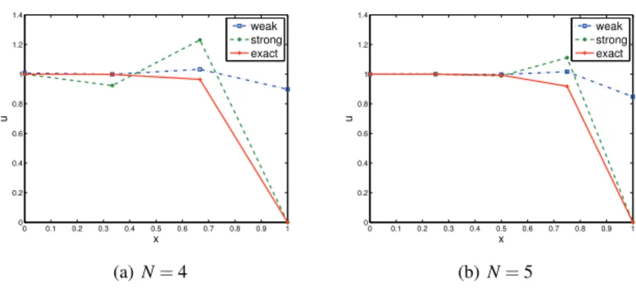
We investigate very coarse meshes and take N = 4 and N = 5 and compare the weak, strong and exact solutions in Figure 2.2. The weak solution is more accurate than the strong solution for all points except precisely at the boundary (where we know the solution anyway). The weak method gently enforces the right boundary condition as the grid is refined.

Next, we consider the flow on a flat plate and study the development of the boundary layer subject to boundary data from the Blasius similarity so-lution [33]. A Mach number of 2 and a Reynolds number of 10000 is used. We solve the compressible Navier-Stokes equations using second- and fourth-order schemes with weak and strong boundary conditions on different meshes.

(19)

0 0.1 0.2 0.3 0.4 0.5 0.6 0.7 0.8 0.9 1 0 0.2 0.4 0.6 0.8 1 1.2 1.4 x u weak strong exact (a) N = 4 0 0.1 0.2 0.3 0.4 0.5 0.6 0.7 0.8 0.9 1 0 0.2 0.4 0.6 0.8 1 1.2 1.4 x u weak strong exact (b) N = 5

Figure 2.2: The weak, strong and exact solutions for a = 1,ε = 0.1.

Stretched meshes are used in the y-direction near the plate to capture the boundary layer features.

Boundary conditions on velocities u, v and temperature T are implemented weakly to obtain a solution referred as the weak solution. We also implement strong boundary conditions on u and v while T remains weakly imposed. This is referred to as the strong solution. We integrate in time until we reach steady-state. The numerically computed solutions are compared to the Blasius simi-larity solutions in Figure 2.3 where we have shown normalized velocity and temperature using a fourth order scheme and a fine mesh.

−0.20 0 0.2 0.4 0.6 0.8 1 1.2 5 10 15 20 25 30 35 40 45 u/u_e y/L Tabulated weak BC, 4th−order scheme strong BC, 4th−order scheme

0.9 1 1.1 1.2 1.3 1.4 1.5 1.6 1.7 1.8 0 5 10 15 20 25 30 35 40 45 T/T_e y/L Tabulated weak BC, 4th−order scheme strong BC, 4th−order scheme

Figure 2.3: Navier-Stokes and similarity solutions, 4th order scheme,∆xmin= 0.001,

∆ymin= 0.0001.

As we have already seen for the model problem, the weak solution behaves like an advection solution on coarse meshes. Similar features could be ob-served also for the Navier-Stokes equations, see Figure 2.4. Moreover, the weak solution has the same asymptotic convergence rate as the strong solu-tion for fine meshes. We notice that as the mesh is refined, the weak boundary conditions force the solution from a slip (Euler) condition to a no-slip (Navier-Stokes) condition.

(20)

−0.20 0 0.2 0.4 0.6 0.8 1 1.2 5 10 15 20 25 30 35 40 45 u/u_e y/L Tabulated

weak BC, 2nd−order scheme strong BC, 2nd−order scheme

(a)∆xmin= 0.1,∆ymin= 0.01

−0.20 0 0.2 0.4 0.6 0.8 1 1.2 5 10 15 20 25 30 35 40 45 u/u_e y/L Tabulated

weak BC, 2nd−order scheme strong BC, 2nd−order scheme

(b)∆xmin= 0.05,∆ymin= 0.005

Figure 2.4: The weak boundary condition goes from a slip (Euler) to a no-slip (Navier-Stokes) condition.

2.2 Paper II

The SAT technique is normally applied only at one grid point [14, 32, 34, 35, 36]. However, it is possible to impose the weak boundary conditions at multiple grid points where, for accuracy reasons, the solution must be known. In Paper II, we discuss the possibilities of using this technique.

We consider the problem

ut+ Aux= 0, x∈ [0,1], t > 0,

A+u (0,t) = gL(t) ,

A−u (1,t) = gR(t) ,

(2.7)

together with an initial condition which leads to a well-posed problem [15, 16, 17, 36, 37]. A is an m× m symmetric matrix that can be split according to the sign of its eigenvalues as A = A++ A−. The extended penalty regions [0,ε0]

and [ε1, 1] are shown in Figure 2.5. Note that we are interested in computing

the solution in the region [ε0,ε1] and that we already know it in [0,ε0] and

[ε1, 1].

Figure 2.5: Illustration of extended penalty regions [0,ε0] and [ε1, 1].

(21)

Table 2.1: Convergence rates for uniformly 4th and 6th order schemes.

Points 4th order scheme 6th order scheme l2-error q l2-error q 21 4.10e− 04 − 6.60e− 06 − 41 2.64e− 05 3.95 1.18e − 07 5.80 81 1.66e− 06 3.99 2.02e − 09 5.87 161 1.03e− 07 4.00 3.29e − 13 5.93 321 6.48e− 09 4.00 5.26e − 13 5.96 0 10 20 30 40 50 0 1 2 3 4 5 6 7 N min|real( )|

Standard penalty term One additional penalty term Two additional penalty terms Three additional penalty terms

Figure 2.6: The effect of adding penalty terms on more grid points to the spectrum. The min|real(λ)| is shown for various N.

The error equation for the problem (2.7) is given by et+

(

P−1Q⊗ A)e =(P−1⊗ I)(R0+ Rmul) e + Te. (2.8)

Here R0is the standard SAT penalty term and Rmul an additional penalty term

operating in the extended regions. Te is the truncation error and⊗ denotes the Kronecker product. Using the energy method on (2.8) (with Te = 0) lead to

d dt∥e∥ 2 P+ eT [( Q + QT)⊗ A]e = eT[R0+ RT0 + Rmul+ RTmul ] e. (2.9)

For stability reasons we choose Rmul+ RT_mul ≤ 0. Other demands on Rmul will

(22)

0 100 200 300 400 500 10−15 10−10 10−5 100 t Norm of error t=500.00, N=11, 21, 41 N=11, SP N=11, MP N=21, SP N=21, MP N=41, SP N=41, MP

Figure 2.7: Rate of convergence to steady-state using standard and multiple penalty terms, N = 11, 21, 41. SP: Standard Penalty, MP: Multiple Penalty.

0 0.2 0.4 0.6 0.8 1 −0.5 0 0.5 1 1 Initial Solution region Penalty region 0 0.2 0.4 0.6 0.8 1 −5 0 5 x 10−3 Domain x u−v

Error moves with speed = 2a

Figure 2.8: Error propagation with speed 2a in the penalty region.

If the difference operator P−1Q is a uniformly high order difference oper-ator with the same order of accuracy everywhere in the domain including the boundary region, then Q + QT ̸= B and additional terms compared to the stan-dard SBP case are obtained. However, we can choose Rmul such that the error

in (2.9) is bounded. The raised accuracy of the uniformly high order schemes for the system (2.7) is shown in table 2.1.

To increase the rate of convergence to steady-state, we can use Rmulto

mod-ify the incoming and outgoing waves. It gives us the option to modmod-ify the

(23)

spectrum as shown in Figure 2.6 for various number of grid points, N = 6 to N = 41.

The convergence rate to steady-state of the new scheme compared with the standard SBP scheme is shown in Figure 2.7 for N = 11, 21, 41. Another possibility is to choose the parameters in Rmul such that we can increase the

wave speed of the errors, see Figure 2.8. We can also combine the different techniques and lower the wave speed in the penalty region and damp the re-flections at the same time, see Figure 2.9.

0 0.2 0.4 0.6 0.8 1 −5 0 5x 10 −3 aR +_{=1, a} R −_{=1, c} 0=0.00 Error 1 w_1n−w_1e w_2n−w_2e (a) 0 0.2 0.4 0.6 0.8 1 −5 0 5x 10 −3 a_R+ =0.5, a_R− =0.5, c₀=1.00 Error 1 w_1n−w_1e w_2n−w_2e (b)

Figure 2.9: Non-reflecting properties for the 4th order SBP scheme. (a) SBP scheme and standard penalty term, (b) The error wave speed is modified and damping is added in the penalty region [0.75, 1]. N = 101 and t = 0.4.

(24)

2.3 Paper III

In Paper III, we develop a scheme suitable for flow fields where both shocks and smooth solutions exist. By using specific smooth functions, we switch between higher and lower order schemes in different regions.

Consider the unsteady one-dimensional conservation law

ut+ f (u)x= 0, 0≤ x ≤ 1, t ≥ 0. (2.10)

The second order discretization of (2.10) using the MUSCL approach [38] results in Ut+ 1 ∆x ( F_i+1 2− Fi−12 ) = 0. (2.11)

A second order discretization of the flux function in (2.10), obeying the SBP property and with the introduction of the artificial dissipation [22] leads to

Ut+ D2F =−P−1D˜T1BMD˜1U, (2.12)

where D2 is a central second order finite difference operator. It can be shown

that the matrix BM can be constructed such that (2.12) corresponds to the

standard second order MUSCL formulation given in (2.11). The matrix eD1is

a two point difference operator and the matrix BM is a diagonal,

e D1=       −1 1 −1 1 . .. ... −1 1      , BM=       b0 0 b1 . .. 0 bN      . (2.13) The matrix BM is a function of U and for stability it must be positive

semi-definite.

We construct a hybrid scheme which is based on high order SBP operators and the MUSCL scheme on SBP form. With the help of smooth diagonal matricesΦ and Ψ, we propose a hybrid scheme (ignoring the dissipation term in (2.12) ) of the form

Ut+ (Dp+Φ(D2− Dp) + (D2− Dp)Ψ)F(U) = 0, (2.14)

where the subscripts on the matrix D denote the order of the approximation. D is a difference operator on SBP form. We need a stable and conservative procedure that switches the higher order scheme to a second order scheme and vice versa. In combination with the low order scheme, we activate the MUSCL scheme in the region of discontinuity or shock. If Ψ = Φ, then the scheme defined in (2.14) can be proven to be both conservative and energy stable. For example, ifΨ = Φ = 0 we get a higher order scheme, and if Ψ = Φ = 0.5, we get a lower order scheme.

(25)

We investigate the hybrid scheme by considering a non-linear flux function ( f = u2/2) with u(x, 0) = sin(2πx) as initial data. We compare the hybrid scheme with the MUSCL scheme at t = 0.15. A comparison of the l2-errors

for successively refined meshes is made in table 2.2, and clearly the hybrid scheme is more accurate.

Table 2.2: l2-error, at T=0.15.

Points 21 41 81 161 321

Hybrid scheme 0.0242 0.0114 0.0040 0.0015 0.0006 MUSCL scheme 0.0349 0.0139 0.0049 0.0018 0.0006

2.4 Paper IV

As a continuation of Paper III, a procedure to locally change the order of ac-curacy of finite difference schemes is developed. The development is based on existing SBP operators and a weak interface treatment. The resulting scheme is accurate, conservative, and stable.

To explain our technique we consider the scalar advection equation

ut+ aux= 0, −1 ≤ x ≤ 1. (2.15)

We introduce an interface at x = 0, such that uL_t + auL_x = 0 holds in the left domain (−1 ≤ x ≤ 0) and uR_t + auR_x = 0 holds in the right domain (0≤ x ≤ 1). The interface condition is uL(0,t) = uR(0,t). The resulting numerical approx-imation of (2.15) is

vL_t + aP_L−1QLvL=τLPL−1eN(vLN− vR0)

v_tR+ aP_R−1QRvR=τRP_R−1e0(vR₀− vLN),

(2.16)

in the left and right domain, respectively and whereτLandτRare the penalty

coefficients, e0= [1, 0, . . . , 0], eN = [0, . . . , 0, 1] and N is the number of grid

points. The equations in (2.16) is rewritten as

Vt+ a ¯P−1QV = ¯¯ P−1TV,¯ (2.17)

where we have defined:

V= [ vL vR ] ¯ P= [ PL 0 0 PR ] ¯ Q= [ QL 0 0 QR ] ¯ T= [ τLeNeTN −τLeNeT0 −τRe0eTN τRe0eT0 ] .

(26)

The vector V in (2.17) has two elements representing the solution u at the interface. By matrix manipulations, (2.17) is transformed into a scheme with a single-valued interface. The derived scheme is

Wt+ a eP−1QW = 0,e (2.18)

where W is a new solution vector, that is one element shorter than V . Further, e

P = ePT > 0 and eQ is skew-symmetric in the interior. To be precise eQ≡ eI¯QeIT and eP≡ eI¯PeIT, where eI is defined in (2.19).

eI=             1 . .. 1 0 0 0 0 1 1 0 0 0 0 1 . .. 1             (2.19)

The new scheme (2.18) possesses all the SBP properties, which automatically leads to a conservative and stable scheme.

Consider the time-independent problem ux= S(x) with boundary condition

u(0) = g0, having u(x) = sin(7x)− cos(4x) as the manufactured solution. We

solve this equation using the adjustable scheme e

P−1QW = S +e τ eP−1e0(w0− g0), (2.20)

where e0= [1, 0,··· ,0]T and S is the discrete representation of S(x) such that

Si≡ S(xi). As penalty parameter we useτ = −1. The scheme in (2.20) changes

order at iL= N/4 and iR = 3N/4, such that it is second order accurate for

0.25 < x < 0.75 and fourth order outside this interval. The resulting solution and error (using N = 32 and N = 64) are shown in Figure 2.10.

In Figure 2.11 the errors from these simulations are visualized. If the pro-portions of lower (2nd) and higher (4th or 6th) order points in the scheme do not change, the overall order of accuracy is the lower (2nd) one. If the number of 2nd order points in the scheme remains constant as the mesh is refined we obtain third order accuracy, for both the 4th and 6th order schemes. This is consistent with the theory in [24].

The most obvious application for this methodology is simulations of prob-lems with discontinuous solutions. For the scalar one-dimensional conserva-tion law ut+ Fx= 0, we use the scheme,

Wt+ eP−1QF =e −eP−1DT1BeMD1W, (2.21)

which we refer to as the hybrid scheme. The hybrid scheme (2.21) shifts from a 4th order accurate scheme away from the discontinuity to the second order

(27)

0 0.2 0.4 0.6 0.8 1 −1 0 1 2 x Solution u,v u, exact v, N=32 v, N=64 (a) Solution 0 0.5 1 −0.01 0 0.01 0.02 x Error e=v − u v−u, N=32 v−u, N=64 (b) Error

Figure 2.10: For 0.25. x . 0.75 the scheme is 2nd order accurate, while it is 4th

order accurate outside.

102 103

10−8

10−6

10−4

10−2

Number of grid points, N

Error, L 2 (v − u) P 424, iL=N/4, iR=3N/4 P 424, iL=N/2−8, iR=N/2+8 P 626, iL=N/4, iR=3N/4 P 626, iL=N/2−8, iR=N/2+8 Slope=−2 Slope=−3

Figure 2.11: The l2norm of the error as a function of the number of grid points, N.

The amount of lower order points in the scheme is either increasing with N or held constant.

accurate scheme close to the shock where the MUSCL dissipation is added on. We study the advection equation with F = u, u(0,t) = g0(t) and u(x, 0) =

u0(x) as a combination of a Gaussian pulse and a step function as the initial

solution, i.e.

u0(x) =

{

e−100(x−0.2)2+ 1, 0≤ x ≤ 0.6 0.5, 0.6 < x≤ 1.

This means that the solution has both smooth and discontinuous parts. In Fig-ure 2.12 the solutions and errors from the hybrid scheme are compared to the ones from the WENO and MUSCL schemes. We observe that both the

(28)

MUSCL scheme and the WENO scheme cut the top of the Gaussian pulse. The hybrid scheme does not. Close to the discontinuity, the solutions for all three schemes are similar.

0 0.2 0.4 0.6 0.8 1 0.5 1 1.5 2 x u Initial Exact WENO3 MUSCL Hybrid (a) Solution 0 0.2 0.4 0.6 0.8 1 !0.2 !0.15 !0.1 !0.05 0 0.05 0.1 0.15 0.2 x error WENO3 MUSCL Hybrid (b) Error

Figure 2.12: Solution and error. Comparison between the WENO scheme, the MUSCL scheme and the hybrid scheme. N = 80 and t = 0.15.

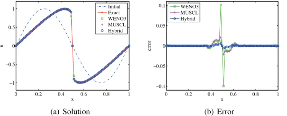
Next, we consider the nonlinear Burgers equation, i.e. F = u2/2 with a sine wave as initial condition, u0(x) = sin(2πx). In Figure 2.13 the simulations at

time t = 0.186 are shown. This is after a shock has formed. The hybrid scheme produces a solution that is more accurate than the ones from the MUSCL scheme and the WENO scheme.

0 0.2 0.4 0.6 0.8 1 !1 !0.5 0 0.5 1 x u Initial Exact WENO3 MUSCL Hybrid (a) Solution 0 0.2 0.4 0.6 0.8 1 !0.1 !0.05 0 0.05 0.1 x error WENO3 MUSCL Hybrid (b) Error

Figure 2.13: Solution and error from the WENO scheme, the MUSCL scheme and the hybrid scheme. After time t = 0.16 the MUSCL dissipation is turned on in the hybrid scheme. Time t = 0.186 and N = 80.

(29)

2.5 Paper V

The MUSCL scheme [38] is a very effective approach to capture disconti-nuities. In Paper V, we discuss the energy stability of the standard MUSCL scheme. The analysis is possible by reformulating the MUSCL scheme in the form (1.6). As we have already discussed the reformulation in Section 2.3, we start with (2.12), which we write as

Ut+ P−1QF =−P−1D˜T1BMD˜1U. (2.22)

where P−1Q is a second order SBP operator and P−1D˜T₁BMD˜1U is an artificial

dissipation term. The matrices BM = diag(b0, b1, . . . , bi, . . . , bN) and ˜D1 are

defined in (2.13).

In this work, we consider two versions of energy stability. The scheme defined by (2.22) is said to be pointwise energy stable if bi ≥ 0 for all i =

0, 1 . . . , N, where N is the number of grid points. The scheme defined by (2.22) is said to be energy stable in the mean if (DU )TBM(DU )≥ 0, where

DU = [(DU )0, (DU )1, . . . , (DU )N]T.

The MUSCL scheme depends on the slope limitersϕ, which are used to avoid the non-physical oscillations that would otherwise occur with high order spatial discretization close to discontinuities. From the theory of slope limiters [39] for a second order total variation diminishing scheme, we find that 0≤ ϕ ≤ 2 is required. 0 50 100 150 200 −1 −0.5 0 0.5 1 min(b i ) / time step

Number of time steps

(a) min(bi) per time step

0 50 100 150 200 −0.6 −0.5 −0.4 −0.3 −0.2 −0.1 0

dissipation / time step

(b)−(D1U )TBM(D1U ) 0 0.2 0.4 0.6 0.8 1 0.5 1 1.5 2 x solution vector Initial soluton Numerical solution Exact solution (c) solution, N = 80, t = 0.3

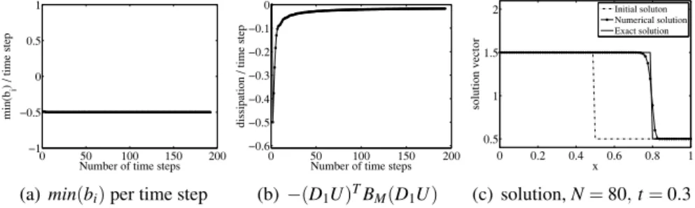
Figure 2.14: Results from the MUSCL scheme in SBP form using the minmod lim-iter, f = u.

First we consider a linear problem ( f = u) with a step discontinuity as initial data and analyze the four different limiters minmod, Van Leer, su-perbee and MC. We compute −(D1U )TBM(D1U ) and the minimum of bi

at each time step. The minmod limiter was found to have bi ≥ 0 for the

whole time and hence it is pointwise stable as shown in Figure 2.14. All other limiters led to bi < 0 at a few points near the discontinuity. These limiters

were not pointwise stable. In Figure 2.15, we show the minimum of bi and

−(D1U )TBM(D1U ) at each time step for the Van Leer limiter. It was also

found that −(D1U )TBM(D1U )≤ 0 for all limiters for the whole

(30)

0 50 100 150 200 −1 −0.5 0 0.5 1 min(b i ) / time step

0 50 100 150 200 −0.6 −0.5 −0.4 −0.3 −0.2 −0.1 0

Figure 2.15: Results from the MUSCL scheme in SBP form using the Van Leer limiter, f = u. 0 50 100 150 200 −1 −0.5 0 0.5 1 min(b i ) / time step

0 50 100 150 200 −0.6 −0.5 −0.4 −0.3 −0.2 −0.1 0

Figure 2.16: Results from the MUSCL scheme in SBP form using the minmod lim-iter, f =u₂2. 0 50 100 150 200 −1 −0.5 0 0.5 1 min(b i ) / time step

0 50 100 150 200 −0.6 −0.5 −0.4 −0.3 −0.2 −0.1 0

Figure 2.17: Results from the MUSCL scheme in SBP form using the Van Leer limiter, f =u₂2.

Next we considered the Burgers equation with f = u2/2 in (2.10) and re-peated the same analysis. It was found that nearly all the tested limiters have some values of bi< 0. However, the minmod limiter gives biwhich is zero for

whole times leading to pointwise stability. Results are shown for the minmod and Van Leer limiters in Figures 2.16 and 2.17 respectively. The results show that the Van Leer limiter is not pointwise stable, while the minmod is both pointwise and energy stable in the mean.

(31)

It is currently not clear whether pointwise stability is necessary or if sta-bility in the mean suffice for good performance. If we replace bi < 0 in the

matrix BMwith bi= 0 at each time step to make it point-wise stable, we found

that it lead to an additional and excessive amount of dissipation in the discon-tinuity/shock region. By demanding pointwise stability, clearly the sharpness of the shock decreases.

2.6 Paper VI

In Paper VI, we apply most of the techniques discussed previously to a de-manding flow case involving both boundary layers and shocks. The particular case considered was a Mach 1.5 shock wave diffracting over a 30◦ convex wall. A hybrid technique was demonstrated in which a higher order code was made locally first order in the immediate vicinity of the shock wave. This pro-vided numerical stability close to the shock while retaining the higher order accuracy everywhere else in the flow field. In all cases the same mesh was used and the Reynolds number was varied from Re = 20 000 to Re = 400 000. The shock capturing method in the code was verified against a standardized benchmark test of a shock wave diffracting over a backward facing 30◦wedge [40]. The code is capable of solving the Navier-Stokes and Euler equations with 2nd , 3rd , 4th or 5th order accuracy [41, 36, 32].

The geometry used in the computations and a numerical result is shown in Figure 2.18. As can be seen from the placement of the blocks in Figure 2.18, the computational effort has gone into resolving the flow along the lower wall.

(a) (b)

Figure 2.18: Domain with block boundaries indicated (a.) and a typical result (b.) for

a Mach 1.5 shock diffracting over a 30◦backward facing wedge.

Figure 2.19 illustrates the effect of Reynolds number on the 3rd order results for a shock diffraction over a complex, convex wall. The same mesh, initial and inlet conditions were used for all four simulations, producing a shock at

(32)

the inlet boundary with the same Mach number (Mach 1.5) each time. Only the Reynolds number was increased in each of the computations, effectively reducing the viscosity term in each case.

The most readily noticeable change as the Reynolds number is varied in the results presented in Figure 2.19 is the shape of the weaker features along the shear layer. The formation of a range of weak shocklets in a lambda configu-ration along the shear layer has been very well documented from experimental data. However, resolving the phenomenon numerically has often proven very difficult. The computational results are visualized at a much higher temporal and spatial resolution than is traditionally possible in most shock tubes. The numerical results were compared visually with experimental images [42], and were found to be in good agreement.

(a) (b)

(c) (d)

Figure 2.19: Schlieren images of the hybrid 3rd order solver results with a. Re = 100 000, b. Re = 200 000, c. Re = 400 000 and d. Re = 200 000 for the full domain.

Furthermore, an examination of the velocity profiles at two locations along the lower wall shows that the boundary layer along the wall was adequately re-solved in all calculations. Also, by monitoring the velocities at the solid wall, which is meaningful for the weak treatment, it was shown that the computa-tions were resolved.

In summary, it may not currently be practicable to run a properly resolved direct numerical simulation (DNS) calculation at the Reynolds number of a

(33)

comparable experiment. From the results presented it can however be con-cluded that an adequate solution can be achieved that is resolved in the region of interest and provides results comparable to experiments.

(34)

(35)

3. Summary in Swedish

Partiella differentialekvationer (PDE) används vid modellering av ett flertal processer inom forskning och ingenjörskonst. Exempelsvis fluiders rörelse, värmeöverföring, solidmekanik och biologiska processer. En PDE beskrivas som en ekvation innehållandes en funktion av flera variabler samt deras par-tiella derivator. Ofta faller en PDE inom en av kategorierna hyperboliska-, paraboliska- eller elliptiska PDE:er. Dock kan en del PDE:er tillhöra fler än en kategori. Till exempel så besitter advektion-diffusionsekvationen egenskaper som är både hyperboliska och paraboliska.

För att en PDE ska vara väldefinierad krävs rand- och initialvillkor. En PDE som utrustats med både rand- och initialvillkor kallas för ett initial-randvärdesproblem. Vilka initial- och randvilkor som är lämpliga för en PDE är ett högst icke-trivialt problem. Fokuset i den här avhandlingen ligger på PDE:er som beskriver tidsberoende fluid- och vågutbredningsproblem.

För att numeriskt kunna lösa PDE:er krävs, förutom initial- och randvil-lkor för den kontinuerliga PDE:n, en korrekt behandling av dessa vilrandvil-lkor för den numeriska beräkningsmetoden. En uppsjö av olika metoder finns tillgäng-liga, till exempel finita differenser, finita volymer, finita element och spektrala metoder.

I den här avhandlingen har vi analyserat noggrannhets- och stabilitetsaspek-ter för svaga rand- och gränssnittsvillkor (SRV) vid användandet av högre ordningens finita differensoperatorer på partiell summations-form (PS). Effek-tiviteten och användbarheten har undersökts då de svaga villkoren appliceras både vid randpunkterna samt även vid ett antal inre punkter i beräkningsdomä-nen. Vi har konstruerat hybridmetoder som gör det möjligt att gå från hög till låg noggrannhet i närheten av stötar. Arbetet i avhandlingen avslutas med högupplösta stötberäkningar för strömmningsfall som innehåller gränsskikt där den framarbetade teorin kommer till full användning.

Den stora fördelen med SRV framför stark implementering av randvillkor är att stabilitet för det numeriska schemat kan bevisas. Vi diskuterar svag och stark randvillkorsbehandling för advektion-diffusionsekvationen där vi har tillgång till analytiska lösningar. Den tidsoberoende ekvationen kan lösas exakt och lösningen beskriver ett gränsskikt vid den ena randen. De teoretiska resultaten appliceras på Navier-Stokes ekvationer och vi kan numerisk visa att slutsatserna för modellproblemet gäller även för gränsskikten som bildas vid lösningen av Navier-Stokes ekvationer.

(36)

Traditionellt har de svaga randvillkoren applicerats enbart vid beräknings-domänens randpunkter. I många fall vet man dock vad lösningen ska vara även en liten bit in i domänen. Genom att utnyttja detta faktum har vi konstruerat SRV som sträcker sig ett givet antal beräkningspunkter in i beräkningsdomä-nen. Resultatet är att noggrannheten hos lösningen i närheten av randen kan höjas, konvergenshastigheten mot den tidsoberoende lösningen kan ökas sam-tidigt som ofysikaliska reflektioner från ränderna kan minskas.

För stötproblem är det viktigt med en metod som inte bara är stabil utan även konservativ. Stabilitet (tillsammans med konsistens) ger konvergens, och vice versa, för linjära och välställda problem via Lax berömda ekvivalenste-orem. För stötproblem är detta dock inte tillräckligt för att erhålla en nog-grann metod. Korrekt stöthastighet kan enbart garanteras om beräkningsmeto-den även är konservativ. Genom att kombinera differensoperatorer på PS-form med SRV har vi konstruerat två olika konservativa och energistabila hybrid-metoder för stötproblem.

I den första hybridmetoden har vi kombinerat en högre ordningens finit dif-ferensmetod på PS-form med en andra ordningens noggrann MUSCL-metod. MUSCL-metoden har omformulerats inom ramverket för PS och lags till som en artificiell dissipation, vilket används för att bevisa energistabilitet för den första hybridmetoden. För de klassiska gradientkontrollerna (eng. slope lim-iters) visade vi även att den resulterande artificiella dissipationen inte är neg-ativt semidefinit, vilket krävs för punktvis energistabilitet.

För att använda en finit differensmetod för stötproblem får den enligt Go-dunovs teorem vara maximalt första ordningens noggrann för att inte orsaka oscillationer. Ett problem som innehåller både reguljära områden och stötar är således svårt att beräkna. I den andra hybridmetoden har vi utvecklat en metod för att lokalt ändra beräkningsmetodens noggrannhetsordning i närheten av stötar. Ett problem som innehåller både snälla områden och stötar kan således behandlas på ett uniformt sätt med den andra hybridmetoden.

Som avslutning på avhandlingen har vi utfört högupplösta stötberäkningar där den framarbetade teorin har omsatts i praktik. Gränsskiktet bakom stöten vid fasta väggar har studerats för olika Reynolds-tal och jämförts med Schlieren-bilder för ett motsvarande experiment. De högupplösta beräkningarna visade fler intressanta fenomen som de expermentiella resultaten inte var kapabla att fånga, men som teoretiskt borde existera.

(37)

4. Acknowledgments

I humbly thank Allah Almighty, the Compassionate, the Merciful, who gave health, thoughts, affectionate parents, talented teachers, caring family, help-ing friends and an opportunity to contribute to the vast body of knowledge. Peace and blessing of Allah be upon the Holy Prophet MUHAMMAD (peace be upon him), the last prophet of Allah, who exhort his followers to seek for knowledge from cradle to grave and whose incomparable life is glorious model for the humanity.

I would like to express my sincere gratitude towards my advisor, Professor Jan Nordström, for his inspiring and valuable guidance, enlightening discus-sions, kind and dynamic supervision through out in all the phases of this thesis. I have learnt a lot from him and working with him has been a pleasure.

I sincerely thank all the co-authors namely, Craig Law, Sofia Eriksson, Per Pettersson and Edvin van der Weide for their valuable contribution in the ar-ticles included in this thesis. Thanks also to Kenneth, Per and Anna for their support in writing this thesis. Jens and Sofia, thanks for writing the Swedish summary and proof reading.

Higher Education Commission (HEC) of Pakistan is gratefully acknowl-edged for the financial support and Swedish Institute (SI) for coordinating the scholarship program. Uppsala University is also gratefully acknowledged for partial support.

A special thanks goes to all the members of the department of Informa-tion Technology of Uppsala University for their help and cooperaInforma-tion. I really enjoyed working here. Many thanks to Tom Smedsaas, Carina Lindgren, and Marina Nordholm for their help during this period. Jukka Komminaho and Tore Sundqvist are acknowledged for their technical support in making our codes run on the UPPMAX.

I owe many thanks to my fellow PhD students in Uppsala University for their encouragement and support. Special thanks to my country friends and their families in Uppsala for arranging great get-togethers. I would also like to thank all my relatives and friends in Pakistan for always being in contact with me.

(38)

I am deeply thankful to my parents, parents-in-law, brothers and sister for their endless support and prayers. I am really grateful to my wife Uzma, for her sacrifices and contributions during these years. Finally, to my daughters, Hadia, Hania and Aribah for giving me a lot of motivation and happiness, making everything meaningful.

Qaisar Abbas, Uppsala, Sweden October, 2011

(39)

Bibliography

[1] J. A. Trangenstein. Numerical Solution of Hyperbolic Partial Differential Equa-tions. Cambridge University Press, New York, 2009.

[2] S. Abarbanel and A. E. Chertock. Strict stability of high-order compact implicit finite-difference schemes: The role of boundary conditions for hyperbolic PDEs, I. Journal of Computational Physics, 160(1):42–66, 2000.

[3] S. Abarbanel, A. E. Chertock, and A. Yefet. Strict stability of high-order com-pact implicit finite-difference schemes: The role of boundary conditions for hy-perbolic PDEs, II. Journal of Computational Physics, 160(1):67–87, 2000. [4] M. H. Carpenter, D. Gottlieb, and S. Abarbanel. The stability of numerical

boundary treatments for compact high-order finite-difference schemes. Journal of Computational Physics, 108(2):272–295, 1993.

[5] D. W. Zingg. Comparison of high-accuracy finite-difference methods for linear wave propagation. SIAM Journal of Scientific Computing, 22(2):476–502, 2000. [6] Bo Strand. Summation by parts for finite difference approximations for d/dx.

Journal of Computational Physics, 110(1):47–67, 1994.

[7] H. O. Kreiss and G. Scherer. Finite element and finite difference methods for hyperbolic partial differential equations. In Mathematical Aspects of Finite El-ements in Partial Differential Equations; Proceedings of the Symposium, pages 195–212. Academic Press, Inc. New York, 1974.

[8] H. O. Kreiss and G. Scherer. On the existence of energy estimates for difference approximations for hyperbolic systems. Technical report, Uppsala University, 1977.

[9] M. H. Carpenter, J. Nordström, and D. Gottlieb. A stable and conservative inter-face treatment of arbitrary spatial accuracy. Journal of Computational Physics, 148:341–365, 1999.

[10] K. Mattsson and J. Nordström. Summation by parts operators for finite differ-ence approximations of second derivatives. Journal of Computational Physics, 199(2):503–540, 2004.

[11] M. H. Carpenter, D. Gottlieb, and S. Abarbanel. Time-stable boundary con-ditions for finite-difference schemes solving hyperbolic systems: methodology

and application to high-order compact schemes. Journal of Computational

(40)

[12] P. Olsson. Summation by parts, projections, and stability, I. Mathematics of Computation, 64(211):1035–1065, 1995.

[13] P. Olsson. Summation by parts, projections, and stability, II. Mathematics of Computation, 64(212):1473–1493, 1995.

[14] K. Mattsson. Boundary procedures for summation-by-parts operators. Journal of Scientific Computing, 18(1):133–153, 2003.

[15] J. Nordström and M. H. Carpenter. Boundary and interface conditions for high-order finite-difference methods applied to the Euler and Navier-Stokes equa-tions. Journal of Computational Physics, 148(2):621–645, 1999.

[16] J. Nordström and M. H. Carpenter. High-order finite difference methods, multi-dimensional linear problems, and curvilinear coordinates. Journal of Computa-tional Physics, 173(1):149–174, 2001.

[17] B. Gustafsson. High Order Difference Methods for Time Dependent PDE.

Springer-Verlag Berlin Heidelberg, 2008.

[18] B. Gustafsson, H. O. Kreiss, and J. Oliger. Time dependent Problems and Dif-ference Methods. Wiley-Interscience, New York, 1995.

[19] Bo Strand. Numerical studies of hyperbolic ibvp with high-order finite differ-ence operators satisfying a summation by parts rule. Applied Numerical Mathe-matics, 26(4):497–521, 1998.

[20] J. Nordström and M. Björck. Finite volume approximations and strict stability for hyperbolic problems. Applied Numerical Mathematics, 38:237–255, 2001. [21] J. Nordström, K. Forsberg, C. Adamsson, and P. Eliasson. Finite volume

meth-ods, unstructured meshes and strict stability for hyperbolic problems. Applied Numerical Mathematics, 45:453–473, 2003.

[22] K. Mattsson, M. Svärd, and J. Nordström. Stable and accurate artificial dissipa-tion. Journal of Scientific Computing, 21(1):57–79, 2004.

[23] J. Nordström. Conservative finite difference formulations, variable coefficients, energy estimates and artificial dissipation. Journal of Scientific Computing, 29(3):375–404, 2006.

[24] M. Svärd, J. Gong, and J. Nordström. Stable artificial dissipation operators for finite volume schemes on unstructured grids. Applied Numerical Mathematics, 56:1481–1490, 2006.

[25] R. J. LeVeque. Finite volume methods for hyperbolic problems. Cambridge University Press, Cambridge, 2002.

[26] N. Adamas and K. Shariff. High-resolution hybrid compact-ENO scheme

for shock-turbulence interaction problems. Journal of Computational Physics, 127(2):27–51, 1996.

(41)

[27] B. Costa and W. S. Don. High order hybrid central-WENO finite difference scheme for conservation laws. Journal of Computational and Applied Mathe-matics, 204(2):209–218, 2007.

[28] M.B. Giles. UNSFLO: A numerical method for the calculation of unsteady flow in turbomachinery. Report 205, Gas Turbine Laboratory, MIT, 1991.

[29] D. J. Hill and D. I. Pullin. Hybrid tuned center-difference-WENO method for large eddy simulation in the presence of strong shocks. Journal of Computa-tional Physics, 194:435–450, 2004.

[30] K. Nakahashi and S. Obayashi. FDM-FEM zonal approach for viscous flow computations over multiple bodies. AIAA Paper 1987-0604, January 1987. [31] C. Law, B. W. Skews, and K. H. Ching. Shock wave diffraction over complex

convex walls. In Proceedings of the 26th International Symposium on Shock Waves, Göttingen, Germany, 2008.

[32] M. Svärd and J. Nordström. A stable high-order finite difference scheme for the compressible Navier-Stokes equations: no-slip wall boundary conditions. Jour-nal of ComputatioJour-nal Physics, 227(10):4805–4824, 2007.

[33] F. M. White. Viscous Fluid Flow. McGraw Hill International, 1991.

[34] J. E. Hicken and D. W. Zingg. Parallel Newton-Krylov solver for the Euler equations discretized using simultaneous-approximation terms. AIAA Journal, 46(11):2773–2786, 2008.

[35] X. Huan, J. E. Hicken, and D. W. Zingg. Interface and boundary schemes for high-order methods. AIAA Paper 2009-3658, June 2009.

[36] M. Svärd, M. H. Carpenter, and J. Nordström. A stable high-order finite differ-ence scheme for the compressible Navier-Stokes equations: far-field boundary conditions. Journal of Computational Physics, 225(1):1020–1038, 2007. [37] M. Svärd and J. Nordström. On the order of accuracy for difference

approxi-mations of initial-boundary value problems. Journal of Computational Physics, 218(1):333–352, 2006.

[38] B. Van Leer. Towards the ultimate conservative difference scheme, V. A second order sequel to Godunov’s method. Journal of Computational Physics, 32:101– 136, 1979.

[39] M. H. Berger, M. J. Aftosmis, and S. M. Murman. Analysis of slope limiters on irregular grids. Technical Report NAS-05-007, NAS Technical Report, 2005. [40] K. Takayama and O. Inoue. Shock wave diffraction over a 90 degree sharp

corner - posters presented at the 18th issw. Shock Waves, 1(4):301–312, 1991. [41] J. Nordström, J. Gong, E. van der Weide, and M. Svärd. A stable and

conser-vative high order multi-block method for the compressible Navier-Stokes equa-tions. Journal of Computational Physics, 228:9020–9035, 2009.

(42)

[42] S. Eriksson, C. Law, J. Gong, and J. Nordström. Shock calculations using a very high order accurate Euler and Navier-Stokes solver. In Proceedings of the Sixth South African Conference on Computational and Applied Mechanics, Cape Town, South Africa, 2008.

(43)

(44)