Component-based software development of
multi-mode systems — An extended report
Hang Yin
Chalmers University of Technology, Gothenburg, Sweden yhang@chalmers.se
Hans Hansson
M¨alardalen University, V¨aster˚as, Sweden hans.hansson@mdh.se
Daniele Orlando
University of L’Aquila, L’Aquila, Italy me@danieleorlando.com
Francesco Miscia
University of L’Aquila, L’Aquila, Italy fra.miscia@gmail.com
Simone Di Marco
University of L’Aquila, L’Aquila, Italy simonedimarco89@gmail.com
November 13, 2016
Abstract
Growing software complexity is an increasing challenge for the soft-ware development of modern embedded systems. A classical strat-egy for taming the software complexity is to partition system behav-iors into different operational modes specified at design time. Such a multi-mode system can change behavior by switching between modes at runtime. Component-Based Software Engineering (CBSE) is a com-plementary approach to the software development of complex systems that fosters reuse of independently developed software components. CBSE and the multi-mode approach are fundamentally conflicting in that component-based development conceptually is a bottom-up ap-proach, whereas partitioning systems into operational modes is a top-down approach. In this report we show that it is possible to combine and integrate these two fundamentally conflicting approaches. The key to simultaneously benefitting from the advantages of both approaches lies in the introduction of a hierarchical mode concept that provides a conceptual linkage between the bottom-up component-based approach
and system level modes. As a result, systems including modes can be developed from reusable mode-aware components in the model-ing phase. The conceptual drawback of the approach—the need for extensive message exchange between components to coordinate mode switches—is eliminated by an algorithm that collapses the component hierarchy and thereby eliminates the need for inter-component coordi-nation. As this algorithm is used from the design to implementation level (“compilation”), the CBSE design flexibility can be combined with efficiently implemented mode handling. At the more specific level, this report presents (1) a mode mapping mechanism which formally specifies the mode relation between composable multi-mode compo-nents, (2) a mode transformation technique that transforms component modes to system-wide modes to achieve efficient implementation, and (3) a prototype tool that implements the mode mapping mechanism and mode transformation technique.
1
Introduction
Growing software complexity is posing a challenge for the software design of embedded systems. A common practice to manage software complexity is to partition system behaviors into different mutually exclusive operational modes so that each mode corresponds to a specific system behavior. Such a multi-mode system [1] usually runs in one mode and can switch to another mode under certain conditions. For instance, the control software of an airplane could run in the modes taxi (the initial mode), taking off, flight and landing. Multi-mode systems have also been motivated by many other reasons:
1. More efficient software design, testing, and verification. A multi-mode system allows for the separate design and parallel testing of different modes, thus facilitating system development.
2. Diversity of system functionality. A multi-mode system exhibits dis-tinctive functionalities in different modes. Therefore, it is usually easier for a multi-mode system to provide more diversified services compared to a single-mode system.
3. Adaptivity. A multi-mode system can be considered as a type of adap-tive system that acadap-tively adjusts its behavior and performance to ac-commodate new conditions. For instance, an adaptive media player of an embedded device with constrained resource may switch between the degraded Quality of Service (QoS) mode and normal mode, depending on available runtime resources.
4. Saving resources. For those systems with a lot of tasks which only need to run under certain conditions, the constant running of all tasks
would be a waste of resources. It is more efficient to deactivate the tasks that are not currently used in the system. Different modes could be specified based on the set of running tasks.
5. Fault tolerance. Most safety-critical systems are designed to be fault-tolerant so as to reduce the risks for catastrophic consequences. A practical fault-tolerant strategy is to switch to a safe mode in case a fault occurs.
6. More precise analysis of system properties. Many system properties are associated with a wide range of values, however, the maximum and minimum could have extremely low probability of occurrence. A typical example is the Worst-Case Execution Time (WCET) of a task in a real-time system. The WCET calculation is typically rather pes-simistic because it is often much larger than the average-case execution time. If a task runs in multiple modes, its WCET can be calculated or measured for each mode, thereby yielding more precise WCET es-timates.
7. Extensibility and scalability. For a single-mode system, adding a new function risks polluting the software structure of the original system and necessitates the test of the complete new system. Alternatively, if a new mode is introduced for the new function, the system behavior in existing modes will not be affected. Additional development and test effort is limited to the new mode and the mode switch from or to this new mode. This also implies good scalability of a multi-mode system. As a complementary approach to multi-mode systems, Component-Based Software Engineering (CBSE) [2] advocates the reuse of independently developed software components as a promising technique for development of complex software systems. The success of CBSE has been evidenced by a variety of component models proposed both in industry and academia [3, 4]. CBSE suggests software modularity and reusability to facilitate the develop-ment of high-quality software. For instance, different functional modules or even subsystems of the control software of an airplane can be encapsulated into reusable software components which can be reused multiple times for the same system or for other systems in the same software product line.
Applying CBSE in multi-mode systems or the other way round has been a largely unexplored research area, possibly because multi-mode systems and CBSE are fundamentally conflicting in the sense that the former tradi-tionally is a top-down approach, whereas the latter is a bottom-up approach. Our research goal in this report is to despite this apparent conflict combine these approaches and benefit from the advantages of both multi-mode sys-tems and CBSE. Hence, we propose component-based software development of multi-mode systems, characterized by the independent development and
reuse of multi-mode components (i.e., components which can run in multiple modes) in the system modeling phase.
1.1 A guiding example
As a guiding example, consider a proof-of-concept healthcare monitoring system. The system consists of two subsystems: Data Acquisition Sub-system and Monitoring SubSub-system. The Data Acquisition SubSub-system uses cameras and microphones to collect video and audio data from a ward or a private home. The data is encoded, encrypted, and transmitted to the Monitoring Subsystem over a reliable network. The data arriving at the Monitoring Subsystem is decrypted, decoded, and reported to the health center. Video and audio data are decoded separately. The video is dis-played on a screen, while the audio is dis-played by a speaker. The Monitoring Subsystem also includes an alarm which is triggered when the person being monitored encounters a dangerous situation, such as falling or suffering from a heart attack.
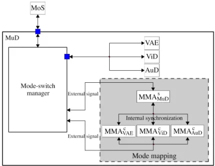
Our focus is on the software architecture of the Monitoring Subsystem (MoS), which is composed by multi-mode components. The component structure of the system is modeled and illustrated in Fig. 1 where its com-ponent hierarchy is presented on the left and comcom-ponent connections are depicted on the right. The system is represented by Component MoS at the top level, composed by three subcomponents: DaD for data decryption, the multimedia decoder MuD, and EvA for event analysis. Due to the tree structure of the component hierarchy, DaD, MuD, and EvA are also called the children of MoS, which consequently is their parent. The system can run in two different modes: Regular monitoring mode (denoted as Rm) and Attention mode (denoted as Att ).
The system runs in mode Rm if nothing special happens to the healthcare target. This mode has very low requirement on video resolution and there is no need to transmit audio data. Hence it is assumed that only video data is transmitted and a fast video encoding/decoding algorithm is used to provide medium video quality which can be maintained by low CPU and bandwidth usage. Shown in Fig. 1, the video data from the network is first decrypted by DaD and then decoded by MuD, which sends the decoded video data to the display in the health center. Represented by the dimmed color, EvA is deactivated when MoS runs in Rm. Meanwhile, DaD runs in a Regular mode R1, while MuD runs in a Regular decoding mode Rd. The internal structure of MuD for mode Rd is also depicted in Fig. 1. MuD consists of three subcomponents: VAE for video/audio extraction, a video decoder ViD and an audio decoder AuD. While MuD runs in Rd, ViD is its only activated subcomponent running in a Regular video decoding mode Rvd, since MuD receives only decrypted video data.
Figure 1: The architectural model of a mode system built from multi-mode components
subsystems will switch to an Attention mode Att. This mode intends to raise the attention of the health center. Both video and audio data are expected to be transmitted. Moreover, the video resolution should be higher, thus requiring a different encoding/decoding algorithm. Component EvA is activated, running in a Regular mode R2, to analyze the detected event and may trigger an alarm when necessary. Due to the growing video data size and the additional audio data, the network load will be substantially increased. Depending on the current network condition, MuD may run in an Enhanced decoding mode Ed or a Degraded QoS mode Dq. Under satisfying network conditions, MuD runs in Ed, with all its subcomponents activated. The subcomponent VAE runs in a Regular mode R3, separating decrypted video and audio data and sending them to ViD and AuD, respectively. To produce higher quality video, the video decoder ViD runs in an Enhanced video decoding mode Evd by applying a different video decoding algorithm. This is represented by the grey color of ViD in Fig. 1. The audio decoder AuD runs in a Regular audio decoding mode Rad. However, if the network condition deteriorates to a certain level, it may become unsuitable to transmit both video and audio data. A possible strategy is to skip the transmission of audio data to maintain the video quality which could be more important. As a result, MuD switches to the mode Dq, in which AuD is deactivated to skip audio decoding. When the network condition returns to normal, MuD will automatically switch back to Ed. Note that VAE only receives video
data while MuD runs in Dq. This implies that VAE can be deactivated in the same way as AuD. However, VAE remains activated when MuD runs in Dq to avoid frequent activation and deactivation. Without audio data, VAE simply forwards the video data to ViD.
We distinguish two types of components in the Monitoring Subsystem: primitive components and composite components. DaD, EvA, VAE, ViD, and AuD are primitive components which are directly implemented by code, while MoS and MuD are composite components composed by other com-ponents. What makes this system distinctive compared with traditional component-based systems is its constitution of multi-mode components.
1.2 Contributions
In achieving the component-based software development of multi-mode sys-tems, this report includes the following key contributions:
• A mode mapping mechanism for mapping component modes during the composition of multi-mode components. This mechanism uses Mode Mapping Automata (MMA) to locally map the modes of a com-posite component to the modes of its subcomponents at design time. The mechanism partially builds on the MMA in [5], which are sub-stantially refined, including detailed specification of MMA syntax and execution semantics, as well as formal definition of MMA composition. • A mode transformation technique that transforms component modes to system-wide modes to achieve efficient implementation. This is obtained by flattening the hierarchical structure of component modes mapped at different levels. Mode transformation can be included in the mapping from the design to implementation level (“compilation”), after the mode mappings of all composite components in a system have been specified. An initial version of the mode transformation technique is presented in [6].
• A prototype tool, MCORE—the Multi-mode COmponent Reuse En-vironment, which implements both the mode mapping mechanism and the mode transformation technique for building multi-mode systems with multi-mode components. MCORE is implemented as a prepro-cessor for the commercial component-based development environment Rubus ICE [7], and thus extends Rubus ICE, which supports system level modes only, with the ability to benefit from reusable multi-mode components.
Mode mapping elegantly links modes and software component reuse. The hierarchical composition of multi-mode components easily allows one to build multi-mode systems with multi-mode behaviors at various levels.
A potential drawback of this approach is the runtime overhead due to inter-component communication for coordination of the mode switches of different components. To eliminate this runtime drawback, while still being able to design systems from reusable multi-mode components we introduce mode transformation, which enables efficient centralized mode management of a multi-mode system while preserving the flexible reuse of multi-mode com-ponents.
The rest of this report is structured as follows: Section 2 elaborates on the composition of multi-mode components and the mode mapping mecha-nism. Section 3 presents the mode transformation technique. The prototype tool MCORE is described in Section 4. Related work is reviewed in Section 5. Finally, Section 6 concludes the report and discusses some future work.
2
The composition of multi-mode components
As an essential step in the composition of multi-mode components, mode mapping unambiguously specifies the mode relation between different multi-mode components at design time. This section highlights the essential prop-erties of multi-mode components and the motivation of mode mapping, fol-lowed by a thorough explanation of Mode Mapping Automata (MMA), i.e., a formal description of mode mapping, as well as MMA composition.
2.1 Multi-mode components and mode mapping
In general, a multi-mode component supports multiple modes and has a unique configuration defined for each mode. Fig. 2 illustrates the key prop-erties of a reusable multi-mode component. The configuration for each mode relies on various factors. For instance, a multi-mode primitive compo-nent may have different mode-specific behaviors for different modes; while a multi-mode composite component may have different set of subcomponents activated depending on its mode.
A multi-mode component can switch between certain modes at runtime, either on its own initiative or passively as requested by another component. A mode switch leads to the reconfiguration of the component by changing its configuration in the current mode to a new configuration in the target mode. A local mode-switch manager is used to handle the mode switch of a multi-mode component. By having such a mode-switch manager in each component, a multi-mode component is able to exchange mode information with its parent and subcomponents via dedicated mode-switch ports (the blue ports in Fig. 2) during a mode switch even without knowing the global mode information. We have previously developed distributed mode-switch algorithms [8, 9] running in the mode-switch manager for the cooperative mode switch of different components.
Since we assume that multi-mode components are independently devel-oped, they typically support different number of modes and name them differently. It is necessary to specify the relation between the modes of dif-ferent components at design time without ambiguity. Such a specification is called mode mapping. To ensure reusability, the mode mapping must never violate the following principles:
• A primitive component knows the mode information (supported modes, initial mode and current mode) of itself, but knows nothing about the other components in the system.
• A composite component knows the mode information of itself and its immediate subcomponents, but knows nothing about the other com-ponents in the system.
Hence, it is the responsibility of each composite component to map its own modes to the modes of its subcomponents, whereas mode mapping is not needed for a primitive component. Tables 1 and 2 present the basic mode mappings of composite components MoS and MuD of the example in Fig. 1. Modes in the same column are mapped to each other. For instance, when MoS runs in mode Att, among its subcomponents, DaD runs in R1, MuD can run in either Ed or Dq, and EvA runs in R2. These tables intuitively present a set of mode mapping rules within MoS and MuD. However, there are some other mode mapping rules which are beyond the description of both tables. For example, when MoS switches from Rm to Att, according to Table 1, MuD may switch to either Ed or Dq. To eliminate such non-determinism, one of Ed and Dq must be specified as the default target mode of MuD. To be able to formally specify all types of mode mapping rules, we came up with a more powerful presentation—Mode Mapping Automata.
Before going into the details of the Mode Mapping Automata, we would like to point out that it is not our intention to develop a complete theory for a new type of automata. Rather, our focus is to, based on established
Table 1: The mode mapping table of MoS Component Modes MoS Rm Att DaD R1 MuD Rd Ed Dq EvA Deactivated R2
Table 2: The mode mapping table of MuD
Component Modes
MuD Rd Ed Dq
VAE Deactivated R3
ViD Rvd Evd
AuD Deactivated Rad Deactivated
automata concepts, provide a formalization of mode mapping that suits our specific purposes.
2.2 Mode Mapping Automata
Let c be a composite component with SCc being the set of subcomponents
of c and Pcbeing the parent of c. When c is running in one of its supported
modes, it should always know its current mode and the current modes of all ci ∈ SCc by its mode mapping, which can be presented by mode mapping
tables such as Table 1. Moreover, whenever the mode-switch manager of c notices the mode switch of ci ∈ SCc∪ {c}, it will refer to the mode mapping
which should tell which other components among SCc∪{c}\{ci} should also
switch mode as a consequence, and the new modes of these components. The complete mode mapping of c can be formally presented by a set of MMA, which consist of one Mode Mapping Automaton of c (denoted as MMAsc) and one MMA of each subcomponent ci ∈ SCc(denoted as MMAcci).
Here we call MMAsc a self MMA and MMAcci a child MMA.
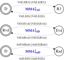
As an example, Fig. 3 presents the set of MMA of the component MuD in Fig. 1, including a self MMA (MMAsMuD) and three child MMA (MMAcVAE, MMAcViD, and MMAcAuD). These MMA are hierarchically organized in the same way as the corresponding components. Each MMA can receive and emit internal or external signals. Internal signals are used to synchronize the pair of the self MMA and its child MMA while external signals interact with its local mode-switch manager for requesting and returning mode mapping results. As shown in Fig. 2, a multi-mode component can exchange mode-related information with its parent and subcomponents via its dedicated
mode-switch ports. Every time MuD receives a mode-switch request from its parent MoS or a subcomponent via a dedicated mode-switch port, its mode-switch manager will send an external signal to the set of MMA to derive the modes of MuD and the modes of its subcomponents.
Figure 3: The role of the mode mapping of MuD at runtime A self or child MMA can be formally defined as follows:
Definition 1. Mode Mapping Automaton (MMA): An MMA is de-fined as a tuple:
hS, s0, SI, T i
where S is a set of states; s0 ∈ S is the initial state; SI = I ∪E (I ∩E = ∅) is a set of signals received or emitted during a state transition, with I as the set of internal signals and E as the set of external signals; T ⊆ S × SI × 2SI× S is a set of transitions of the MMA.
In addition to the formal definition above, an MMA can be graphically represented as a state machine with states and transitions. Each state is represented by a circle, with the initial state being marked by a double circle. If the MMA is a self MMA of c, then each state corresponds to a mode of c. If the MMA is a child MMA of c associated with ci ∈ SCc, then
each state corresponds to a mode of ci or the deactivated status of ci, if ci
can be deactivated, denoted as D. A transition t ∈ T is represented by an arrow from a state s to a state s0, denoted as s−−−−→ sIn/Out 0, where In/Out is
the label of the transition, “In” is the input that triggers the transition and “Out” is the output of the transition.
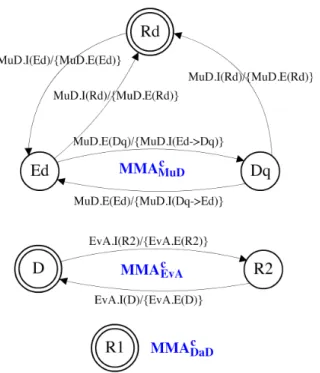
Fig. 4 depicts MMAsMuD, i.e, the self MMA of MuD of the example in Fig. 1. Three states are included in this MMA, implying that MuD can run in three modes. The state transitions of MMAsMuD and the corresponding child MMA MMAcVAE, MMAcViD, and MMAcAuD (later shown in Fig. 5) are manually specified to determine the mode mapping of MuD. Shown in Fig. 4, each transition has a label with input and output separated by “/”. The input and output of a transition are typically internal and external signals. We define two types of internal signals and a single type of external signal denoted as follows:
• x.I(y), an internal signal emitted by a self MMA to the recipient MMAcx, which is asked to change state to y.
• x.I(z → y), an internal signal emitted by MMAcx which requests to change state from z to y.
• x.E(y), an external signal asking MMAx, which is either a self MMA
or a child MMA, to change state to y.
Figure 4: The self Mode Mapping Automaton of MuD
Note that an internal signal emitted from a self MMA to a child MMA is in the form of x.I(y), while an internal signal emitted from a child MMA to a self MMA is in the form x.I(z → y). A self MMA of a composite component a sends an internal signal b.I(mb) to a child MMA MMAcb when
the mode mapping of a wants b to switch to a new mode mb, regardless of
the current mode of b. In contrast, the reason for using x.I(z → y) instead of x.I(y) in the latter case is that both the current mode and the target mode of a component can affect the mode mapping result of its parent.
In order to get a self MMA synchronized properly with the corresponding child MMA, the set of MMA of a composite component c must fulfill several
constraints regarding their transitions. We define the constraints by taking the following principles into account:
• The mode mapping of c is determined by its self MMA, not any child MMA.
• The input of the set of MMA must be an external signal which is either the input of MMAsc (if the mode switch is initiated by c) or the input of a child MMA MMAcci, where ci is a subcomponent of c (if the mode
switch is initiated by ci).
• The output of the set of MMA must be either a set of external signals (if the input external signal implies the mode switch of at least another component in SCc∪ {c}) or an empty set otherwise.
• The internal synchronization between MMAs
c and the child MMA is
based on only internal signals. There is no direct synchronization between child MMA.
• An internal signal from MMAscto a child MMA MMAcci only needs to indicate the new mode of ci, while an internal signal from MMAcci to
MMAsc needs to indicate both the current mode and new mode of ci,
as both parameters affect the mode mapping results of MMAsc. • Usually the starting state and ending state of a transition in an MMA
should be different. However, there is one exception in MMAsc. If the mode switch of a subcomponent ci does not imply the mode switch of
c, this will result in a transition in MMAsc starting and ending in the same state.
The principles above yield the following constraints applied to both self and child MMA:
1. For the self MMA MMAsc, the input of each transition must be either an external signal c.E(mc) or an internal signal ci.I(m1ci → m
2
ci), where
mc is the target mode of c of the transition, ci ∈ SCc, and m1ci and
m2ci are the modes of ci. Then,
(a) If the input is c.E(mc), then the output is either an empty set or
a set of internal signals in the format ci.I(mci), where ci ∈ SCc
and mci is the target mode of ci.
(b) If the input is ci.I(m1ci → m
2
ci), then the output is a set with two
parts. The first part is an external signal c.E(mc) if the starting
state of this transition is different from the ending state mc, or
an empty set otherwise. The second part is either an empty set or a set of internal signals in the format ci.I(mci), where ci∈ SCc
2. For each child MMA MMAcci, where ci is a subcomponent of c, if it
has only one state, then there is no transition in MMAcci. If MMAcci has at least two states, then the starting state and ending state of each transition must be different. For each transition to the state mci,
the input must be either an external signal ci.E(mci) or an internal
signal ci.I(mci). If the input is ci.E(mci), then the output must be an
internal signal ci.I(m0ci → mci) where m
0
ci is the current mode of ci;
if the input is ci.I(mci), then the output must be an external signal
ci.E(mci).
3. For each internal signal ci.I(mci) in the output of a transition of
MMAsc, there must be one and only one transition of MMAcci with the input ci.I(mci), synchronized with this transition of MMA
s
c and
vice versa. For each internal signal ci.I(m0ci → mci) in the output of
a transition of MMAcci, there must be one and only one transition of MMAsc with the input ci.I(m0ci → mci), synchronized with this
transi-tion of MMAcci and vice versa.
Following the constraints above, we specify the MMA synchroniza-tion semantics as follows: Let c be a composite component with SCc =
{c1
i, c2i, · · · , cni} (n ∈ N). Let A = {A0, A1, · · · , An} be the set of MMA of
c, with A0 associated with c and Ak associated with cki (k ∈ [1, n]). Hence
A0 is the self MMA while the others are child MMA. Any external signal from the mode-switch manager of c at runtime can potentially lead to the MMA synchronization of c. An MMA synchronization is an atomic transac-tion which is always performed between A0 and the other child MMA. The
synchronization depends on if the external signal arrives at A0 or at a child
MMA:
1. An external signal arrives at A0 asking c to switch to mode mc. This
triggers a transition t of A0 with the input c.E(mc), giving rise to two
possible subsequent events:
• The mode switch of c under this condition does not imply the mode switch of any subcomponent of c. Then the output of the transition t is an empty set ∅, i.e. there is no internal synchro-nization between the set of MMA of c and no external signals are expected to be emitted from them to the mode-switch manager of c.
• The mode switch of c under this condition implies the mode switch of at least one of its subcomponents. Let G ⊆ SCc be
the set of its subcomponents which also need to switch mode. Then the output of t is a set R such that for each cki ∈ G which is expected to switch to the mode mck
signal cki.I(mck
i) ∈ R, synchronizing t with the transition ti with
the label cki.I(mck i)/c
k
i.E(mck
i) of the child MMA Ai. The output
cki.E(mck
i) of ti is sent from Ai to the mode-switch manager of c
which will inform cki to switch to mode mck i.
2. An external signal arrives at Ak (k ∈ [1, n]) asking cki to switch from
mode m1 to m2. This triggers a transition tk of Ak with the label
ck
i.E(m2)/cki.I(m1 → m2), synchronized with the transition t of A0
with the input cki.I(m1→ m2). The output of t may give rise to four
possible subsequent events: • The mode switch of ck
i under this condition does not imply the
mode switch of any component among c and SCc\ {cki}. Then
the output of t is ∅ and no further synchronization and external signal are expected.
• The mode switch of ck
i under this condition implies the mode
switch of c but not the mode switch of any other subcomponent of c. Let mc be the new mode of c. Then the output of t is
c.E(mc).
• The mode switch of ck
i under this condition implies the mode
switch of at least another subcomponent of c but not the mode switch of c. Then the subsequent event will be the same as the second case under Condition (1). Hence the output of t is the set R.
• The mode switch of ck
i under this condition implies the mode
switches of both c and at least another subcomponent of c. Let mc
be the new mode of c. Then the output of t will be {c.E(mc)}∪R,
where c.E(mc) is an external signal emitted from A0.
Our MMA synchronization semantics is partially illustrated by Fig. 4 and Fig. 5 which provide the graphical presentations for MMAsMuD and the corresponding child MMA.
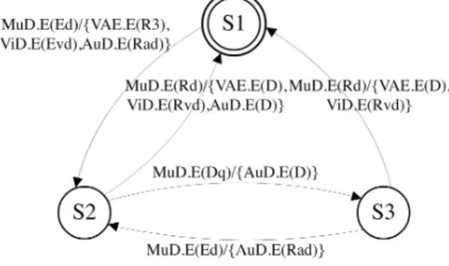
We assume that MoS can initiate a mode switch between Rm and Att, while MuD can initiate another mode switch between Ed and Dq. Let’s use one scenario to demonstrate the synchronization between MMAsMuD and the child MMA. Suppose that MoS initiates a mode switch from Rm to Att due to the detection of a dangerous situation reported to the health center, leading to the mode switch of MuD from Rd to Ed as a consequence. Then the mode-switch manager of MuD is sup-posed to send an external signal MuD .E(Ed ) to MMAsMuD, triggering the transition Rd −−−−−−−−−−−−−−−−−−−−−−−−−−−−−−−−→ Ed of MMAMuD .E(Ed )/{VAE .I(R3 ),ViD .I(Evd ),AuD .I(Rad )} s
MuD,
MMAcVAE, Rvd −−−−−−−−−−−−−−−−−→ Evd of MMAViD .I(Evd )/{ViD .E(Evd )} c
ViD, and the
transi-tion D −−−−−−−−−−−−−−−−−−→ Rad of MMAAuD .I(Rad )/{AuD .E(Rad )} cAuD. The external signals VAE .E(R3 ), ViD .E(Evd ), and AuD .E(Rad ) will be sent to the mode-switch manager of MuD, which will inform VAE, ViD, AuD to mode-switch mode to R3, Evd, and Rad, respectively.
Figure 5: The child Mode Mapping Automata of MuD
Similarly, Fig. 6 and Fig. 7 display the set of MMA of MoS which replace Table 1, including MMAsMoS, MMAcDaD, MMAcMuD, and MMAcEvA. To sim-plify the graphical presentation of a self MMA, if multiple transitions share the same output, starting and ending states, we combine them into one tran-sition where their different inputs are separated by the notation “||”. For instance, MMAsMoS in Fig. 6 has two transitions Att −−−−−−−−−−−−→ AttMuD .I(Ed →Dq)/∅ and Att −−−−−−−−−−−−→ Att , which are combined into one transitionMuD .I(Dq→Ed )/∅ Att−−−−−−−−−−−−−−−−−−−−−−−−→ Att .MuD .I(Ed →Dq) || MuD .I(Dq→Ed )/∅
An interesting phenomenon that deserves particular attention is the dis-tinction between MMAsMuD in Fig. 4 and MMAcMuD in Fig. 7. The former is a self MMA included in the mode mapping of MuD, while the latter is a child MMA included in the mode mapping of MoS.
Figure 7: The child Mode Mapping Automata MMAcMuD, MMAcEvA, and MMAcDaD
2.3 MMA composition
The internal synchronization between a set of MMA of a composite com-ponent is actually invisible to the mode-switch manager of this composite component. What the mode-switch manager sees is the composition of these MMA. For each composite component, the basic idea of deriving its MMA composition is to analyze the possible outputs of a set of MMA for each possible input from the mode-switch manager. According to the MMA syn-chronization semantics, an external signal from the mode-switch manager of a composite component may give rise to six possible subsequent events with respect to the internal MMA synchronization and the output of the set of MMA. All these six cases must be taken into account in defining the MMA composition.
Also, note that the MMA composition will be defined to suit our purposes only, i.e., it is not a general composition that can be used to compose any set of MMA. Instead, it is only applicable for composition of a single self MMA with a non-empty finite set of child MMA, where these MMA are required to satisfy all the constraints we impose on these types of MMA. As a consequence the composition cannot be further composed using our composition.
el-ements of sets are indexed such that we by the indexing can identify the MMA that a specific element is related to, and x[i] will be used to denote the element of x indexed with i.
Definition 2. MMA composition: For a set A = {A0, A1, · · · , An}(n ∈
N) of MMA, where A0 = hS0, s00, SI0, T0i corresponds to a self MMA and
∀k ∈ [1, n], Ak = hSk, s0k, SIk, Tki correspond to the child MMA
synchro-nized with A0, the MMA composition of A is an MMA defined by the tuple
hS, s0, SI, T i where S ⊆ S0× S1× · · · × Sn s0 = (s00, s01, · · · , s0n) SI = S i∈[0,n] Ei
S and T are the least sets satisfying: (1) s0 ∈ S
(2) If
∃s = (s0, s1, · · · , sn) ∈ S ∧ s0 e0/O0
−−−−→ s00∈ T0 [An external signal e0 ∈ E0 arrives at A0.]
then
s−−−→ se0/O 0 ∈ T ∧ s0 = (s00, s01, · · · , s0n) ∈ S where O and s0k(k ∈ [1, n]) are defined by the following
• O = S k∈[1,n] Ok • ∀k ∈ [1, n], if ∃sk O0[k]/O 0 k −−−−−−→ s00 k ∈ Tk, then Ok = O0k ∧ s0k = s00k; else Ok= ∅ ∧ s0k = sk. (3) If ∃s = (s0, s1, · · · , sn) ∈ S ∧ si ei/Oi −−−→ s0i ∈ Ti ∧ s0 −−−−→ sOi/O0 00 ∈ T0 [An external signal ei∈ Ei(i ∈ [1, n]) arrives at Ai.]
then
s−−−→ sei/O 0 ∈ T ∧ s0 = (s00, s01, · · · , s0n) ∈ S where O and s0k(k ∈ [1, n], k 6= i) are defined by the following:
• If s0= s00, then O =[ k∈[1,n], k6=i Ok • Else (s0 6= s00), O = {O0[0]} ∪[ k∈[1,n], k6=i Ok • ∀k ∈ [1, n], if ∃sk O0[k]/O 0 k −−−−−−→ s00 k ∈ Tk, then Ok = O0k ∧ s0k = s00k; else Ok= ∅ ∧ s0k = sk.
By Definition 2, a set of MMA is closed under composition. This means that the MMA after composition itself is also an MMA. However, note that the MMA resulting from a composition cannot be further composed by our composition, as it does not qualify as a self or child MMA. Also, the in-tention is obviously that the composed MMA behaves the same as the set of MMA being composed from the perspective of the corresponding mode-switch manager, i.e., for each input external signal from the mode-mode-switch manager, the same set of external signals are output by the composed MMA as by the set of MMA being composed. By Definition 2, for each input ex-ternal signal arriving at either the self MMA or a child MMA, MMA compo-sition merges all the intermediate steps for the internal synchronization and emits all the possible external signals as the output in a single transition. This means that the mode-switch manager receives the same set of external signals before and after MMA composition.
Based on Definition 2, let’s revisit the six cases mentioned by the MMA synchronization semantics:
1. An external signal arrives at A0 and O0 = ∅, when the mode switch
of a composite component implies no mode switch among its subcom-ponents.
2. An external signal arrives at A0 and O0 6= ∅, when the mode switch
of a composite component implies the mode switch of at least one of its subcomponents.
3. An external signal arrives at Ai (i ∈ [1, n]) and O0 = ∅, when the
mode switch of a component c implies no mode switch among its parent and its siblings, i.e. components with the same parent as c.
4. An external signal arrives at Ai (i ∈ [1, n]) and O0 only contains an
external signal e0, when the mode switch of a component only implies
the mode switch of its parent but not its siblings.
5. An external signal arrives at Ai (i ∈ [1, n]) and O0 only contains a set
of internal signals ik(k ∈ [1, n]), when the mode switch of a component
only implies the mode switch of at least one of its siblings but not its parent.
6. An external signal arrives at Ai (i ∈ [1, n]) and O0 contains both e0
and ik(k ∈ [1, n]), when the mode switch of a component implies the
mode switch of both of its parent and at least one sibling.
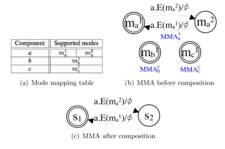
As an example, Fig. 8 demonstrates Case 1 by showing the MMA compo-sition between a composite component a and its two subcomponents b and c. Fig. 8(a) shows the mode mapping table of a, while Fig. 8(b) shows the set of MMA within a. The MMA after composition is shown in Fig. 8(c). Suppose an external signal a.E(m2a) arrives at MMAsa(the self MMA), triggering the transition m1a a.E(m
2 a)/∅
−−−−−−−→ m2
a. Since this external signal does not imply the
mode switch of b or c, no state transition will occur in MMAcb or MMAcc. Let A be the MMA after composition, with two states s1 = (m1a, m1b, m1c) and s2 = (m2a, m1b, m1c). According to Definition 2, A will undergo the transition
s1
a.E(m2 a)/∅
−−−−−−−→ s2.
(a) Mode mapping table (b) MMA before composition
(c) MMA after composition
Figure 8: MMA composition—Case 1
As a more concrete example, consider the MMA composition of MMAsMuD in Fig. 4, MMAcVAE and MMAcViD, and MMAcAuD in Fig. 5. Case 2 is involved in the MMA composition. The composition result is
illus-trated in Fig. 9, where s1 = (Rd , D , Rvd , D ), s2 = (Ed , R3 , Evd , Rad ), and
s3 = (Dq, R3 , Evd , D ).
Figure 9: MMA composition for MuD
2.4 Mode mapping verification
The mode mapping of a composite component specified by MMA can be eas-ily verified by model checking. We use the model checker UPPAAL [10] for mode mapping verification. Since UPPAAL is a convenient tool for modeling and verifying concurrent state transition systems, it is fairly straightforward to graphically model a set of MMA in UPPAAL.
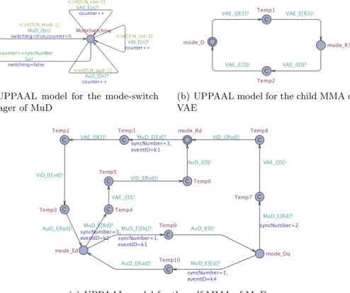
Using UPPAAL, we have modeled1 the mode mapping of MuD specified by the set of MMA in Fig. 4 and Fig. 5. The behavior of the local mode-switch manager of MuD, the self MMA of MuD, and the child MMA of its subcomponents are modeled as separate automata in UPPAAL. For in-stance, Fig. 10 showcases three typical UPPAAL models for the mode-switch manager of MuD, MMAcVAE, and MMAsMuD. Each mode of a component is represented by a state in these UPPAAL models (e.g., mode R3 repre-sents mode R3 in Fig. 10(b)). These models also contain committed states marked with “C” in a circle, which are intermediate states during a mode switch. External and internal signals are simulated as channels synchronized between multiple UPPAAL models. For example, VAE I[R3]! denotes the internal signal VAE.I(R3) emitted by MMAsMuD, while VAE I[R3]? denotes the same signal VAE.I(R3) received by MMAcVAE. The UPPAAL model of MMAsMuD in Fig. 10(c) is consistent with MMAsMuD in Fig. 4. The reason why the UPPAAL model contains one or more intermediate states for each mode switch is that receiving and sending each signal needs to be modeled sequentially in UPPAAL. This essentially does not change the execution se-mantics, as all intermediate states are committed states, whose incoming and outgoing transitions are performed as a single atomic transaction. In
1
The complete UPPAAL model is available at http://www.cse.chalmers.se/~yhang/ JUCS/
addition, shown in Fig. 10(a), the mode-switch manager of MuD consists of two states. InitialS is the initial state, where the mode-switch manager can send an external signal to MMAsMuD and switch to the state ModeSwitch-ing. Meanwhile, a boolean variable switching is set to true, indicating an ongoing mode switch. Depending on the current mode of MuD and the new mode indicated by the external signal from the mode-switch manager, there are four possible events, leading to different transitions among these components: (1) k1: MuD requests to switch from Rd to Ed ; (2) k2: MuD
requests to switch from Ed to Rd ; (3) k3: MuD requests to switch from Ed
to Dq; (4) k4: MuD requests to switch from Dq to Ed. Each event ID is
assigned to a variable eventID as shown in Fig. 10(c).
(a) UPPAAL model for the mode-switch manager of MuD
(b) UPPAAL model for the child MMA of VAE
(c) UPPAAL model for the self MMA of MuD
Figure 10: UPPAAL models of the mode mapping of MuD
Based on the UPPAAL models, we can verify that the set of MMA of MuD satisfy the expected constraints by checking properties formulated in the UPPAAL query language which is a subset of Timed Computation Tree Logic [11]. The following are four types of properties addressing different constraints:
P1. A[] not deadlock : The complete set of UPPAAL models are deadlock-free. This is not directly related to mode mapping, but it is a funda-mental property that we expect the model to satisfy.
P2. E<> sMMA MuD.mode Ed : It is possible for MuD to run in mode Ed. This property should be verified for all the modes of MuD and its subcomponents.
P3. A[] (sMMA MuD.mode Rd and !ModeSwitchManager.switching) imply (cMMA VAE.mode D and cMMA ViD.mode Rvd and cMMA AuD.mode D): When MuD runs in Rd, its subcomponents VAE and AuD must be deactivated while the other subcomponent ViD must run in Rvd. This property should be verified for all possible mode combinations between MuD and its subcomponents according to the mode mapping table in Table 2.
P4. (ModeSwitchManager.switching and eventID==k1)– >(sMMA MuD.mode Ed and cMMA VAE.mode R3 and cMMA ViD.mode Evd and cMMA AuD.mode Rad): An external signal requesting MuD to switch from Rd to Ed will make VAE, ViD, AuD switch to R3, Evd, and Rad, respectively. This property should be verified for all possible events from k1 to k4.
All these properties are satisfied with verification time less than 4ms. Also, our UPPAAL models can be used as a common template for mod-eling any other mode mapping specified by MMA. Due to the graphical resemblance between an MMA and the corresponding UPPAAL model, it is possible to generate UPPAAL models from MMA described by a graphical or textual domain-specific language.
3
Mode transformation
Our previous research results [9] show that the mode switch of a multi-mode component may lead to mode switches of other multi-mode components in the same system and it is not trivial to coordinate the mode switches of different components at runtime. The local mode-switch manager of each component needs to run delicate algorithms to communicate with the parent and subcomponents of the component via dedicated mode-switch ports to switch mode cooperatively. Such inter-component communication incurs runtime computation overhead and mode-switch latency. For instance, when MoS in the healthcare monitoring system triggers a mode switch from Rm to Att, the mode-switch event is first propagated from MoS to MuD and EvA, and MuD subsequently propagates the mode-switch event to VAE, ViD, and AuD. Further, more handshake messages are exchanged between these components to keep mode consistency. The communication overhead grows as the component hierarchy becomes more complex.
The purpose of mode transformation is to eliminate the need for the mode-switch coordination among different multi-mode components by a
centralized mode management, and thereby achieve better runtime perfor-mance, provided that (1) all components are deployed on the same hardware platform, and (2) the mode information of each component is globally acces-sible. lllustrated in Fig. 11, mode transformation transfers the responsibility of mode-switch handling from the local mode-switch manager of each com-ponent to a single global mode-switch manager of the system in the system modeling phase. As a result of mode transformation, each multi-mode com-ponent becomes unaware of modes. Instead, a global mode transition graph is generated for the global mode-switch manager to handle mode switch at system level.
Figure 11: The overview of mode transformation
Our mode transformation process includes two sequential steps. First, given the mode mappings of all composite components, we construct an intermediate representation, a Mode Combination Tree (MCT) where all the possible system modes are identified. In the second step, based on a list of possible mode-switch events defined in the system, we add transitions between the identified system modes to construct the mode transition graph. The two steps are further explained in the following subsections separately.
3.1 Construction of the mode combination tree
The aim of constructing the MCT is to identify all the system modes. Let Mc denote the set of supported modes of a component c and D denote the
current mode of a deactivated component. Then we define system modes as follows:
Definition 3. System modes based on component modes: For a sys-tem composed by a set of components C = {c1, c2, · · · , cn} (n ∈ N), the set
of system modes is defined as Ms⊆
×
i∈[1,n]{Mci∪ {D}}. Each system mode m ∈ Ms is a mode combination of all components.
By Definition 3, each system mode m = (mc1, mc2, · · · , mcn), where
mci ∈ Mci ∪ {D} for i ∈ [1, n]. In order to more explicitly indicate the
ex-pression to represent a system mode: m = {(ci, mci)|i ∈ [1, n]}, where
mci ∈ Mci∪ {D}. Using the same formalism, an MCT is defined as follows:
Definition 4. Mode Combination Tree: An MCT is a tree with a set of nodes N = {N0, N1, · · · , Nn} (n ∈ N), where N0 = ∅ is the root node,
and each other node Ni = {(cj, mcj)|j ∈ [1, k], k ∈ N} (i ∈ [1, n]), where for
all j, mcj ∈ Mcj ∪ {D} and all cj have the same depth level in the system
component hierarchy.
Definition 4 implies that each node of an MCT, except the root node, provides a mode combination of components with the same depth level. A typical outlook of MCT is displayed in Fig. 12, where the construction of the MCT will be further explained.
Before the formal description of the MCT construction process, we need to introduce a number of additional notations and concepts. First, we intro-duce the valid Local Mode Combination (LMC) of a composite component c, which is a feasible combination of a mode of c and the modes of all its subcomponents as per the local mode mapping of c. To formally define the valid LMC of a composite component, let PC and CC be the set of primitive components and composite components in a system, respectively. Let Top be the component at the top of the component hierarchy in a system. For each c ∈ CC, a valid LMC of c is formally defined as follows:
Definition 5. Valid Local Mode Combination: For c ∈ CC with SCc=
{c1
i, · · · , cni} (n ∈ N), we call the set Vc= {(c, mc), (c1i, mc1
i), · · · , (c
n i, mcn
i)}
a valid LMC of c, where mc ∈ Mc∪ {D} and ∀k ∈ [1, n], mkci ∈ Mcki ∪
{D}, if mc and all mck
i (k ∈ [1, n]) can be simultaneously executed by the
corresponding components, i.e. conforming to the mode mapping of c. Note that each element in Vcis a pair (x, y) where x ∈ SCc∪ {c} and y ∈
Mx∪ {D}. For instance, the mode mapping of MoS in Table 1 implies three
valid LMCs of MoS: (1) {(MoS, Rm), (DaD, R1), (MuD, Rd), (EvA, D)}; (2) {(MoS, Att), (DaD, R1), (MuD, Ed), (EvA, R2)}; (3) {(MoS, Att), (DaD, R1), (MuD, Dq), (EvA, R2)}. Actually, each state after MMA composition represents a valid LMC.
Based on Definition 5, we further introduce the valid LMC concerning a specific mode of a composite component c, which is a feasible combination of the modes of all subcomponents of c as per the local mode mapping of c when c is running in a particular mode. A formal definition is given as follows:
Definition 6. Valid LMC concerning a specific mode: For c ∈ CC with SCc = {c1i, · · · , cni} (n ∈ N), if when c is running in mc, and ∀cki ∈
SCc (k ∈ [1, n]), ∃mck i such that {(c, mc), (c 1 i, mc1 i), · · · , (c n i, mcn i)} is a valid
LMC of c, then the set Vc,mc = {(c
1 i, mc1 i), · · · , (c n i, mcni)} is a valid LMC of c for mc.
Depending on the mode mapping of c, multiple valid LMCs of c may exist for mc. Let Wc,mc be the set of all valid LMCs of c ∈ CC for mc.
Each element in Wc,mc is a set Vc,mc. The total number of all valid LMCs
of c for mc is |Wc,mc|. For instance, according to Table 1, WMoS,Att =
{V1
MoS,Att, VMoS,Att2 }, where VMoS,Att1 = {(DaD, R1), (MuD, Ed), (EvA, R2)}
and VMoS,Att2 = {(DaD, R1), (MuD, Dq), (EvA, R2)}. It is easy to automat-ically generate Wc,mc from the mode mapping of c. On the one hand, the
valid LMCs of c for mc can be easily identified from the mc column of the
mode mapping table of c. On the other hand, after MMA composition, each state of the composed MMA represents a valid LMC of c. Then the valid LMCs of c for mc can be easily found in the states with mc. Next we
introduce an important operator for combining different valid LMCs: Definition 7. Valid LMC operation: Consider two sets of valid LMCs W1 = {V1, V2, · · · , Vm} and W2 = {Vk+1, Vk+2, · · · , Vk+n}, where m, n, k ∈
N and k ≥ m. Let ⊕ be an operator such that W1 ⊕ W2 = {Vi∪ Vk+j|i ∈
[1, m], j ∈ [1, n]}. In addition, for each l ∈ N, W1⊕ W2⊕ · · · ⊕ Wl can be
represented as L
o∈[1,l]
Wo.
For the sake of lucidity, let us clarify the ⊕ operator using a small example. Suppose W1 = {V1, V2} where V1 = {(a, m1a), (b, m1b)} and
V2 = {(a, m2a), (b, m2b)}; and W2 = {V3, V4} where V3 = {(c, m1c), (d, m1d)}
and V4= {(c, m2c), (d, m2d)}. Then, W1⊕ W2 ={V1∪ V3, V1∪ V4, V2∪ V3, V2∪ V4} ={{(a, m1a), (b, m1b), (c, m1c), (d, m1d)}, {(a, m1a), (b, m1b), (c, m2c), (d, m2d)}, {(a, m2 a), (b, m2b), (c, m1c), (d, m1d)}, {(a, m2a), (b, m2b), (c, m2c), (d, m2d)}}
Given the component hierarchy of a system and the mode mappings of all composite components in the system, the MCT of the system can be constructed by creating nodes top-down from the root node. For each node N of an MCT, let dN be its depth level, and λN be the number of new nodes
created from this node. We use Ni Nj to denote that a new node Ni is
created from on old node Nj. Moreover, let MTop = {m1T, m2T, · · · , m |MTop|
T }
be the set of supported modes of Top. The MCT is constructed by the following steps:
1. From N0, create λN0 = |MTop| new nodes, such that for each new
node Ni N0, Ni = {(Top, miT)} (i ∈ [1, |MTop|]).
2. From each Ni = {(Top, miT)} (i ∈ [1, |MTop|]), create λNi =
|WTop,mi
T| new nodes, such that for each N
0 N
i, N0 ∈ WTop,mi T.
Moreover, if λNi > 1, then for each N
0, N00 N
3. For each node N = {(c1, mc1), (c2, mc2), · · · , (cn, mcn)} (n ∈ N) with
dN ≥ 2, if ∀i ∈ [1, n], ci ∈ PC, then N is marked as a leaf node and
no new node is created from N . Otherwise, if ∃i ∈ [1, n] such that ci ∈ CC, then create λN = Q
i∈[1,n], ci∈CC
|Wci,mci| new nodes, such that for
each N0 N , N0 ∈ L
i∈[1,n], ci∈CC
Wci,mci. Moreover, if λN > 1, then for each
N0, N00 N , we have N06= N00.
4. Repeat Step 3 until all branches of the MCT have reached the leaf node.
The MCT construction process is implemented as Algorithm 1, which is a recursive function constructMCT (N , dN) that has two input parameters: N
is the node currently being explored and dN is the depth level of N . Initially,
N = ∅ and dN = 0. We assume that Top must have subcomponents.
Otherwise, Top itself will be the entire system and mode transformation will be meaningless. Moreover, for each component c running in mode m, we assume that Wc,m is an indexed set such that Wc,m[i] represents the ith
element of Wc,m.
The complexity of Algorithm 1 depends on the structure of the com-ponent hierarchy, the number of modes of each comcom-ponent, and the mode mappings in the involved components. Since all these contributing factors are bounded, this algorithm will terminate. We have implemented the mode transformation and measured the transformation time (including both steps: deriving the MCT and mode transition graph) for the healthcare monitor-ing system2. The transformation took 2.9-3.9ms. The computation over-head of the algorithm does not affect runtime performance, as the MCT is constructed at design time. The worst-case combination of factors such as number of components and the number of component modes may lead to a huge number of system modes, increasing the overhead exponentially. How-ever, in practice, the expected number of system modes should be limited. If mode transformation becomes intractable due to extreme computation overhead, this would imply that the system is too complex to adopt central-ized mode management. Then it may be more suitable to go for distributed mode management without mode transformation, although especially if the component hierarchy is deep, then the runtime overhead for the required message exchange may be substantial. Alternatively, a better solution could be partial mode transformation, i.e. performing mode transformation within a composite component instead of the entire system. Our mode transforma-tion technique is flexible enough to support partial mode transformatransforma-tion at any component level.
2
Algorithm 1 constructMCT (N , dN) 1: if dN = 0 then 2: λN := |MTop|; 3: for i from 1 to λN do 4: Ni:= {(Top, miT)}; 5: constructMCT (Ni, 1); 6: end for 7: end if 8: if dN = 1 then 9: {(Top, m)} := N ; 10: Derive WTop,m; 11: λN := |WTop,m|; 12: for i from 1 to λN do
13: constructMCT (WTop,m[i], 2);
14: end for 15: end if 16: if dN ≥ 2 then 17: {(c1, mc1), (c2, mc2), · · · , (cn, mcn)} := N ; 18: if ∀i ∈ [1, n] : ci∈ PC then 19: return ; 20: else 21: Derive W := L i∈[1,n], ci∈CC Wci,mci; 22: λN := Q i∈[1,n], ci∈CC |Wci,mci|; 23: for i from 1 to λN do 24: constructMCT (W[i], dN + 1); 25: end for 26: end if 27: end if
As an example, Fig. 12 illustrates the MCT of the monitoring subsystem introduced in Section 1. The MCT consists of 9 nodes N0–N8 with four
depth levels. Represented by the respective paths of the MCT, the three identified system modes are:
m1=N0∪ N1∪ N3∪ N6
={(MoS, Rm), (DaD, R1), (MuD, Rd), (EvA, D), (VAE, D), (ViD, Rvd), (AuD, D)} m2=N0∪ N2∪ N4∪ N7
={(MoS, Att), (DaD, R1), (MuD, Ed), (EvA, R2), (VAE, R3), (ViD, Evd), (AuD, Rad)} m3=N0∪ N2∪ N5∪ N8
={(MoS, Att), (DaD, R1), (MuD, Dq), (EvA, R2), (VAE, R3), (ViD, Evd), (AuD, D)}
Figure 12: The mode combination tree of the monitoring subsystem Since we assume that the Monitoring Subsystem initially runs in mode Rm, m1 is the initial system mode after mode transformation. Fig. 13
shows the configurations of the three system modes based on the component connections in Fig. 1.
An interesting property can be observed from an MCT, formulated as the following theorem:
Definition 8. A non-root node N of an MCT is represented by a valid mode combination of components with depth level dN − 1.
Proof. Since N cannot be the root node, dN ≥ 1. When dN = 1, N =
{(Top, m)|m ∈ MTop} and dTop = dN − 1 = 0. When dN = 2, according
to Step 2 of the MCT construction procedure, N ∈ WTop,m (m ∈ MTop).
The definition of W implies that N is represented by a valid LMC of the subcomponents of Top, while each subcomponent of Top has a depth level dN − 1 = 1. Note that for dN ≥ 3, N is created by the same rule (Step
Figure 13: The configurations of different system modes after mode trans-formation
3). Hence Theorem 8 can be proved by induction for dN ≥ 3. Suppose
N = {(c1, mc1), · · · , (cn, mcn)} (n ∈ N).
Basis: When dN = 3, according to Step 3 of the MCT construction
procedure, the definition of W, and the definition of the operator L, N ∈ L
dci=1 ci∈CC
Wci,mci. Then for all (cj, mcj) ∈ N , dcj = dN − 1 = 2.
Inductive step: Suppose that when dN = k, for all (cj, mcj) ∈ N , we
have dcj = k − 1. Then we need to prove that for another node N
0 = {(c01, mc0 1), · · · , (c 0 o, mc0 o)} (o ∈ N) with dN0 = k + 1, we have dc0i = k (i ∈
[1, o]) for all (c0i, mc0 i) ∈ N
0. The node N0 can be created either from N or
from another node N00with dN00= dN. Since N and N00include the same set
of components with depth level k − 1, we always have N0 ∈ L
dcj=k−1, cj∈CC
Wcj,mcj.
By the definition of W and the operator L, all c0
i included in N0 have a
depth level equal to k, i.e. dN0− 1.
The induction above together with our analysis for dN = 1 and dN = 2
proves Theorem 8.
Theorem 8 further implies the following corollary:
Definition 9. All leaf nodes of an MCT have the same depth level.
Proof. Let N1 and N2 be two leaf nodes of the same MCT. By Theorem 8,
both N1 and N2 include the same set of primitive components with the
of these primitive components. Then d = dN1 − 1 = dN2 − 1. Therefore,
dN1 = dN2, thus proving the corollary.
Once the MCT is constructed, the system modes can be derived as the set of paths from the root node to the leaf nodes of the MCT. Let Nk be the set of nodes of an MCT with depth level k. Then,
Theorem 1. Given an MCT, a system mode m is represented by a valid mode combination
δ
S
i=0
Ni where Ni ∈ Ni is a node representing a valid mode
combination of components with depth level i − 1, Ni+1 is a node created
from Ni, and δ is the maximum depth level of the MCT, i.e. Nδ is a leaf
node. The total number of system modes is equal to the total number of leaf nodes of the MCT.
Proof. Let C = {c1, c2, · · · , cn} (n ∈ N) be the set of components of a system.
First we prove that
δ
S
i=0
Ni includes the modes of all components. Then we
prove that each component is included in m only once. Finally, we prove the valid mode combination as a result of
δ
S
i=0
Ni.
By Theorem 8, each N 6= N0with dN = k is represented by a valid mode
combination of components with depth level k − 1. Since the maximum depth level of the MCT is δ, the maximum depth level of a component in the system is δ − 1. Each path of the MCT is a union
δ
S
i=0
Ni that includes the mode combination of components with depth levels from 0 to δ − 1. Since the depth level of any component is within [0, δ − 1], the mode of the component must be included in
δ
S
i=0
Ni, i.e., a path of the MCT.
Next consider any two pairs (ci, mci) ∈ m and (cj, mcj) ∈ m (i, j ∈ [1, n]).
If dci 6= dcj, then apparently ci 6= cj. If dci = dcj = k, then (ci, mci) and
(cj, mcj) must be both included in any node N ∈ N
k+1 by Theorem 8.
Components ciand cjmay or may not share the same parent. If their parents
are different, then apparently ci 6= cj. If they share the same parent, by
Definition 6, we also have ci6= cj. Therefore, ci6= cj always holds regardless
of the depth levels of ciand cj. Stated otherwise, each component is included
in m only once.
This theorem states that for each i in
δ
S
i=0
Ni, Ni+1 is a node created
from Ni. By Theorem 8 and the MCT construction process, this implies
that Ni ∪ Ni+1 represents a valid mode combination of components with
depth level i − 1 and i. Likewise, at one level down, Ni+1∪ Ni+2represents
a valid mode combination of components with depth level i and i + 1. Hence Ni∪ Ni+1∪ Ni+2 represents a valid mode combination of components with
depth level i, i + 1 and i + 2. By this induction from i = 0 to i = δ,
δ
S
i=0
Ni represents a valid mode combination of all components, i.e., a system mode m.
Furthermore, we know that each path of an MCT includes a leaf node. Since all leaf nodes are different, all paths are also different. The number of paths, i.e. the number of system modes, equals the number of leaf nodes.
Among the system modes, the initial system mode can be recognized based on the specification of the initial modes of all components.
3.2 Deriving the mode transition graph
Once the system modes are identified from the constructed MCT, the next step is to derive the mode transition graph on top of these system modes based on the definition of switch events. We assume that a mode-switch event is triggered by a component c requesting to mode-switch mode m1c to a new mode m2c, denoted as c : m1c → m2
c. The triggering of each
mode-switch event k may lead to the mode mode-switches of some other components in the same system. For a system with a set of identified system modes M = {m1, m2, · · · , mn} (n ∈ N), a mode switch is a transition from moldto mnew,
where mold, mnew ∈ M and mold6= mnew. A mode transition graph contains
all the possible transitions between these system modes and associates each transition with the corresponding mode-switch event. Similar to an MMA, each state of a mode transition graph can be graphically represented by a circle, with the initial state being marked by a double circle. A graphical illustration of mode transition graph can be found in Fig. 14.
The key issue of deriving the mode transition graph is to identify the system modes moldand mnew for each mode-switch event for which a system
mode switch is possible. Consider a mode-switch event k identified as c : m1c → m2
c. The only condition satisfying the triggering of k is that the
triggering source c is currently running in mode m1
c. For each k, mold can
be easily identified as long as (c, m1c) ∈ mold. Note that more than one
system mode could be identified as mold. Depending on the current system
mode, a mode-switch event may enable different transitions.
In contrast to mold, only one system mode can be the mnew for each
mode-switch event k. The identification of mnew for k is more difficult
because it depends not only on m2
c, but also on the target modes of the
other components. We identify the mnew for each mode-switch event with
the assistance of a Component Target Mode (CTM) table. A CTM table is a table with n1rows and n2columns, where n1is the number of components of
a system and n2is the number of mode-switch events. An example of a CTM
table can be found above the mode transition graph in Fig. 14. In the CTM table, each row is associated with a component, each column is associated
with a mode-switch event, and each cell contains the target mode mc of the
corresponding component c for the corresponding mode-switch event k. The cell with X indicates that mc is independent of k.
A CTM table can be automatically constructed offline based on the list of mode-switch events and the mode mapping of each composite component. Let mkcbe the target mode of c for k in a CTM table. Taking advantage of the CTM table, the new system mode mnewfor each mode-switch event k can be
identified as follows: For each system mode m = {(ci, mci)|i ∈ [1, n], n ∈ N},
if ∀i where mkci 6= X in the CTM table (i.e., k leads to the mode switch of ci to a new mode mkci), we have mci = m
k
ci, then m is the mnew for k.
Algorithm 2 describes the process of building the mode transition graph, with a search space of O(|M| · |K|).
Algorithm 2 constructMTG(C, M, K)
1: C = {c1, · · · , co} (o ∈ N); {The set of all components}
2: M = {m1, · · · , mn} (n ∈ N); {The set of identified system modes}
3: K = {k1, · · · , kl} (l ∈ N); {The set of all mode-switch events}
4: for all ki∈ K where k ∈ [1, l] and ki= c : m1c → m2c do
5: if ∃mj∈ M s.t. (∀cp∈ C and mkcpi 6= X, (cp, m ki cp) ∈ mj) then 6: mnew= mj; 7: for all mj∈ M do 8: if (c, m1c) ∈ mj then
9: addTransition(mj, mnew, ki); {Add a transition from mjto mnewlabeled with ki}
10: end if
11: end for
12: end if 13: end for
Fig. 14 presents the workflow for deriving the mode transition graph of the monitoring subsystem. The CTM table is derived based on two inputs: (1) the mode mapping of composite components MoS and MuD specified by MMA, and (2) the possible mode-switch events. For this example, four mode-switch events, from k1 to k4, are specified at design time. k1 and k2
are triggered by MoS for switching between modes Rm and Att, while k3
and k4 are triggered by MuD for switching between modes Ed and Dq. The
target modes of all components in the monitoring subsystem for all mode-switch events are listed in the CTM table. Previously the MCT in Fig. 12 has identified three system modes m1(the initial mode), m2, m3. The CTM
table additionally adds transitions between the system modes based on each possible mode-switch event, thereby yielding the mode transition graph in Fig. 14. The mode transition graph helps the global mode-switch manager to keep track of the current system mode and makes the system switch to the right target mode when a mode switch is triggered.
Using mode transformation, the number of identified system modes is sensitive to the number of modes of each single component and the mode
Figure 14: Deriving the mode transition graph of the monitoring subsystem
mapping of each composite component. As a consequence, mode transfor-mation may end up with a huge number of system modes. Nonetheless, it only makes sense to distinguish one mode from another mode when the system behaviors are noticeably different in these modes. Depending on the application, it could be more efficient to merge several modes with similar global configurations into one mode. For instance, the two system modes m2
and m3 in Fig. 13 are fairly similar to each other, since the only difference
is the activation/deactivation of component AuD. Therefore, it would be more efficient to merge these modes and toggle the status of AuD whenever necessary without mode switch. The criteria for merging system modes are application-dependent and out of the scope of the report. Nevertheless, we believe that it is possible to partially automate the merging of system modes in a later optimization phase by certain application-independent merging rules.
Finally, a potential drawback of mode transformation is the loss of po-tential concurrency between local mode managers. If multiple mode-switch events are triggered concurrently and affect disjoint sets of components, dis-tributed mode management before mode transformation allows that these switch events can be handled concurrently, whereas different mode-switch events have to be sequentially handled by the global mode-mode-switch manager. Nonetheless, the centralized mode management after mode trans-formation eliminates inter-component communication, which is a complex process [9]. Hence mode transformation is still more likely to yield faster mode switch.
3.3 Mode transformation verification
In this section, we verify two key properties of our mode transformation tech-nique in terms of correctness and completeness. First, we need to guarantee that the system modes identified from the MCT are correct and complete. An identified system mode is correct if it is a valid mode combination of the modes of all components as per the mode mapping. The set of identified system modes is complete if it includes all possible system modes as per the mode mapping.
Theorem 2. The system modes identified from the MCT are correct and complete, and each identified system mode is unique.
Proof. Correctness: The correctness is already proven by Theorem 1. Completeness: The completeness of system modes depends on the com-pleteness of the nodes of an MCT. By the MCT construction process, particularly Line 10 and Line 21 of Algorithm 1, whenever we create new nodes from a node N = {(ci, mci)|i ∈ [1, n], n ∈ N}, we consider all the
possible valid LMCs of each ci for mci and all the possible combinations
of their valid LMCs. Hence an MCT has a complete set of nodes which further guarantee a complete set of identified system modes.
Uniqueness: Let m1 and m2 be two different system modes. By Theorem 1,
m1 and m2 correspond to two different paths of the same MCT. Then there
must exist a node N where the two paths diverge. Let N1 and N2 be the
two nodes created from N such that the path of m1 follows N1 and the path
of m2 follows N2. Then N1 and N2 must be different because all new nodes
created from N must be different. Therefore, N1 ∈ m1 and N1 ∈ m/ 2 while
N2 ∈ m2 and N2 ∈ m/ 1, implying that m1 and m2 are unique.
Next we verify the correctness of the mode transition graph, formulated as follows:
Theorem 3. The transitions of a mode transition graph are correct and complete.
Proof. We divide the proof into two parts. First we prove the correctness of the transitions of a mode transition graph. Then we prove the completeness of the transitions of a mode transition graph. Both parts can be proved by contradiction. Let M = {m1, · · · , mn} (n ∈ N) be the set of identified
system modes, where mi, mj ∈ M and k = co: m1co → m
2 co.
To prove the correctness, suppose a mode transition graph contains a wrong transition L = mi
k
−
→ mj (i.e. a transition from mi to mj for k) where
either mi fails to satisfy the triggering condition of k or mj is the wrong
target system mode for k. By Algorithm 2, we know that (co, m1co) ∈ mi.