Image Classification, Deep Learning and Convolutional Neural Networks

(1)

Image Classification, Deep Learning

and Convolutional Neural Networks

A Comparative Study of Machine Learning Frameworks

Rasmus Airola

Kristoffer Hager

Faculty of Health, Science and Technology Computer Science

C-level thesis 15 hp

Supervisor: Kerstin Andersson Examiner: Stefan Alfredsson

(2)

Image Classification, Deep Learning and

Convolutional Neural Networks

A Comparative Study of Machine Learning Frameworks

(3)

Abstract

The use of machine learning and specifically neural networks is a growing trend in software development, and has grown immensely in the last couple of years in the light of an increasing need to handle big data and large information flows. Machine learning has a broad area of ap-plication, such as human-computer interaction, predicting stock prices, real-time translation, and self driving vehicles. Large companies such as Microsoft and Google have already imple-mented machine learning in some of their commercial products such as their search engines, and their intelligent personal assistants Cortana and Google Assistant.

The main goal of this project was to evaluate the two deep learning frameworks Google TensorFlow and Microsoft CNTK, primarily based on their performance in the training time of neural networks. We chose to use the third-party API Keras instead of TensorFlow’s own API when working with TensorFlow. CNTK was found to perform better in regards of training time compared to TensorFlow with Keras as frontend. Even though CNTK performed better on the benchmarking tests, we found Keras with TensorFlow as backend to be much easier and more intuitive to work with. In addition, CNTKs underlying implementation of the machine learning algorithms and functions differ from that of the literature and of other frameworks. Therefore, if we had to choose a framework to continue working in, we would choose Keras with TensorFlow as backend, even though the performance is less compared to CNTK.

(4)

We would like to thank our supervisor from Karlstad University, Kerstin Andersson, for her valuable input and guidance throughout the project. We also would like to thank our super-visors at ÅF Karlstad, Mikael Arvidsson and Daniel Andersson, as well as ÅF Karlstad for giving us this opportunity to learn more about an exciting field of study.

(5)

List of Figures

2.1 Overfitting during training. . . 8

2.2 An artificial neuron. . . 10

2.3 A (simple) artificial neural network. . . 11

2.4 Plot of the sigmoid function. . . 12

2.5 Plot of the rectified linear unit (ReLU) function. . . 13

2.6 A hidden layer of neurons with locally receptive fields. . . 17

2.7 A simple convolutional neural network. . . 19

2.8 An Inception V1 module. . . 21

2.9 A residual block with an ordinary skip connection. . . 22

5.1 Plot of the accuracy for the first run. . . 48

5.2 Plot of the loss for the first run. . . 49

5.3 Plot of the accuracy for the second run. . . 50

5.4 Plot of the loss for the second run. . . 51

5.5 Plot of the accuracy for the third run. . . 52

(8)

List of Tables

5.1 Results CNTK MNIST . . . 47

5.2 Results Keras/TensorFlow MNIST . . . 47

5.3 Results CNTK CIFAR-10 . . . 48

(9)

1 Introduction

This project consisted of roughly 20 weeks of part-time work (three days a week) for the company that gave us the assignment, ÅF Karlstad, more precisely the section for industrial IT. ÅF as a whole is an engineering and consulting company with over 9000 employees which works primarily within the energy, industrial and infrastructure sectors of the economy. The section for industrial IT in Karlstad works primarily with projects concerning production systems in a number of different factories and paper mills.

The primary goal of the project was to evaluate two frameworks for developing and implement-ing machine learnimplement-ing models usimplement-ing deep learnimplement-ing and neural networks, Google TensorFlow and Microsoft Cognitive Toolkit (CNTK). A secondary goal that followed from the first was to explore and learn about deep learning, both the theory and the practice, through the imple-mentation of an image classifier. The evaluation was supposed to consist of as many relevant factors as possible (for more detail see chapters 3 and 4), with the greatest emphasis on the performance of the frameworks in terms of speed and hardware usage. The company’s moti-vation behind the project was to explore the possibility of using machine learning in the work that is being done today regarding production systems and industrial automation, and that led into a need to look into possible tools for development and implementation.

The project thus became a comparative study of the frameworks, a study broken down into parts where different parts were evaluated according to a set of criteria, combined with an exploratory part consisting of learning about deep learning and neural networks through the implementation of an image classifier.

1.1 Project Results

Below a summary of the project results is provided.

At the time of this writing, the frameworks are equal in terms of ease of installation. Regarding setting up the computations on GPU (Graphics Processing Unit), we think the frameworks

(10)

are equal in this regard as well, seeing as they required the same amount of steps and de-pendencies to be installed. When it comes to system requirements and support, the decision which framework is better in this regard largely comes down to which operating system and programming language one is going to use; seeing as CNTK and TensorFlow both support languages the other does not, and that TensorFlow supports Mac OS X and CNTK does not.

We found that the frameworks provide an equivalent set of features and functionalities, and the frameworks are more than capable of constructing neural networks. The frameworks’ documentation were both found to be lacking in both quality and quantity, however Keras has the slight advantage of having its documentation gathered in one place, whereas CNTK has its documentation distributed on different sites. Keras was found to be more beginner friendly and easier to work with, as compared to CNTK. It was found that CNTK does not conform to the literature, having instead its own implementation, which in turn requires relearning if one has studied the literature, it also requires recalculating the parameters in order to function according to the literature; Keras on the other hand, requires no such readjusting, which is a big plus in our view.

CNTK was found to give a shorter training time of the networks compared to Keras with TensorFlow as backend, see tables 5.1-5.4, given the uncertainties listed in chapter 5.3 and the experimental setup presented in chapter 4.3. GPU was found to be so superior over CPU (Central Processing Unit) in terms of training speed, that if one has a GPU available one should use it instead of the CPU. GPU and VRAM (Video RAM) usage were both similar in both CNTK and Keras with TensorFlow as backend.

Regarding the implementation of an image classifier; the model was found to quite rapidly overfit on the training set, a learning rate schedule was found to be beneficial, and the number of epochs seems to have been detrimental to the performance of the model. A number of possible improvements were found and discussed as follows: more regularization, a learning rate schedule with more steps, early stopping, and higher spatial resolution in the latter parts

(11)

of the network.

1.2 Disposition

Chapter 2 will introduce the rationale behind this study and its scope, as well as providing the necessary theoretical background for someone completely new to machine learning to understand the project’s implementation. The deep learning frameworks used in this study will be presented and introduced as well.

Chapter 3 will present an overview of the different parts of the project and the evaluation method used for the different parts. Chapter 3.1 covers the installation and the system re-quirements of the two frameworks and their dependencies; as well as the frameworks’ support of programming languages. Chapter 3.2 covers the frameworks’ features, functionalities and documentation; as well as their support for third-party application programming interfaces, or API:s. Chapter 3.3 covers the frameworks’ performance using two widely used data sets for benchmarking machine learning models; Mixed National Institute of Standards and Tech-nology [1] dataset of handwritten numbers (MNIST) and Canadian Institute for Advanced Research’s dataset of tiny images in color (CIFAR-10) [2]. Chapter 3.4 presents the design of a custom built image classifier.

Chapter 4 will describe the actual implementation of the project’s parts described in chapter 3.

Chapter 5 will present and discuss the results from each part of the evaluation as described in chapter 3 and 4.

Chapter 6 will provide and motivate the conclusion of the evaluation of the frameworks, as well as suggestions for future work, and finally some concluding remarks by the authors.

(12)

2 Background

This chapter will introduce the rationale behind this study and its scope, as well as providing the necessary theoretical background for someone completely new to machine learning to understand the project’s implementation. The deep learning frameworks used in this study will be presented and introduced as well.

Chapter 2.1 will introduce the rationale behind this study and its scope. Chapter 2.2 will provide the necessary theoretical background, where chapter 2.2.1 will focus on deep learning and neural networks, chapter 2.2.2 will focus on convolutional networks, and lastly chapter 2.2.3 will present and discuss different neural network designs and architectures. Chapter 2.3 will present and introduce the deep learning frameworks used in this study. At the end of the chapter a summary is provided.

2.1 Rationale and Scope

In this study the two deep learning frameworks Google TensorFlow and Microsoft Cognitive Toolkit (CNTK) will be evaluated based on their performance and user friendliness. The rationale behind this study is that the company that gave us the assignment wants to integrate machine learning in their work. The company therefore wants to explore the potential of machine learning and to find the best framework to work with (more on such frameworks in chapter 2.3). The motivations for the authors are that machine learning is a very interesting field, in which a lot of possible future breakthroughs in IT can be made, and this study provides a great opportunity to learn more about this field.

Machine learning is a vast field and in order for this study to be completed within the given time span, the scope of the study needs to be limited to some subset of machine learning. The theoretical scope of the study is therefore limited to neural networks, with a focus on convolutional neural networks. The practical scope will be limited to creating and training three equivalent neural networks in both TensorFlow and CNTK for three already prepared and well known datasets in order to evaluate the frameworks’ performance on the same neural

(13)

network. Gathering and preparing training data is therefore beyond the scope of this study. See chapter 3 for further details on the study.

2.2 Machine Learning

Machine learning as a field of research is somewhat hard to describe succinctly, due to the breadth of the field, the amount of ongoing research, the interdisciplinary aspects of the field and a multitude of other factors. For the purposes of this report the following definition will be used as a starting point, as it is sufficiently precise:

"A computer program is said to learn from experience E with respect to some class of tasks T and performance measure P, if its performance at tasks in T, as measured by P, improves with experience E." [3]

From a mathematical standpoint the problem can be formulated as applying a machine learn-ing algorithm to find an unknown mathematical function with a known domain, that of the input, and a known co-domain, that of the output. In more informal terms the program is supposed to find a mathematical connection between the data and the target input. The connection depends on the task at hand. [4] A relevant example of the aforementioned classes of tasks is to find a connection between a vectorized representation of the input to an output consisting of a set of discrete categories or a probability distribution. Concrete examples of such a task can consist of developing a program for image classification and object detection, e.g. recognizing faces in pictures and finding bounding boxes for them. Other examples of types of tasks are anomaly detection, e.g. spotting credit fraud and machine translation, e.g. translation software. [4]

The performance of an implementation of a machine learning algorithm is usually either expressed in the accuracy of the implementation, e.g what percentage of the examples were classified correctly, or in the error rate, e.g what the ratio of incorrectly to correctly classified

(14)

examples is. The difficult part here is not so much the choice of measure rather than which aspect(s) of the output that should be measured in the first place. Should one, for example, choose the percentage of correctly transcribed whole sequences as the only measure or take the correctly transcribed parts of sequences into account when measuring the performance? [4] Another complicating factor is that it can be hard to measure the chosen quantity due to practical difficulties, and in those cases another measure must be chosen.

There are basically two kinds of learning, or experiences, a machine learning algorithm can have during a learning or training process; unsupervised and supervised learning. [4] A training process is based upon a dataset consisting of a given amount of examples or data points. Unsupervised learning is based upon datasets containing features where the goal is to learn useful properties about of the structure of the dataset or, more precisely, to find the underlying probability distribution of the dataset. Supervised learning, in contrast, is based upon datasets consisting of many features but with labels attached to each example. [4] The goal in supervised learning is to learn to predict the label, the associated value, from an arbitrary example in the dataset after the training session is over. The terms supervised and unsupervised comes from the fact that the learning algorithm has a teacher that shows the algorithm what to do in the former case, but is supposed to learn from the data without a guide in the latter case.

The most challenging part of machine learning, regardless of the algorithm(s) applied in the learning process, is to make programs that generalize well; that is, programs that perform as well or almost as well on unobserved inputs as those observed during training. The main thing that separates machine learning from optimization is that the goal consists of minimizing both the training error and the test error. [4] The aforementioned datasets are split in two predetermined sets to be used in the training process, one for training and one for testing. The goal of machine learning can now be defined more precisely; to minimize the training error and to minimize the gap between the training error and the test error. [4] In attempting to achieve the aforementioned goal two more challenges appear; underfitting and overfitting on the training set.

(15)

Underfitting occurs when the model cannot reach a sufficiently low training error and overfit-ting (see figure 2.1) occurs when the gap between the training error and the test error is too large. [4] The former problem is caused by a model with low representational capacity that cannot fit the training set properly, the latter can be caused by a model with high capacity that memorizes properties from the training set too well to perform sufficiently on the test set. [4] Overfitting can also be caused by a training set that is too small to generalize properly from. Underfitting can be fixed rather easily with a model with sufficient capacity, but overfit-ting can be harder to fix due to the fact that acquiring greater amounts of data is not always feasible. A prominent example of a technique that can be introduced during the training is regularization, which is used to limit the space of potential functions (since the goal is to find the best one). [4] There is not much more space to go into detail here, and the problems that can occur and their corresponding solutions will be discussed in later sections.

The parameters of the machine learning algorithm that are not adapted or changed by the algorithm itself during training are called hyperparameters, parameters that can be tuned to change the behavior of the learning algorithm. [4] It is fitting to introduce a further partition of the dataset here, that of the original training data into a training set and a validation set. The training set is used purely for adjusting the internal parameters, e.g weights and biases (see chapter 2.2.1), during the training and the validation set is used to measure the current generalization error and to adjust the hyperparameters accordingly. The validation set is not used to tune the internal parameters. [4] The important distinction between the validation set and the test set is that the latter is not used during the training process at all and does not give any input to the training process - it is simply used to measure performance.

As a final observation in this chapter; there are a lot of machine learning algorithms to choose from, far to many to describe in detail here or even to give a cursory oversight. Since the frameworks in the study are implementations of the components, the functionality and the algorithms necessary to train neural networks and implement deep learning there is no need

(16)

Figure 2.1: Overfitting during training.

As seen in the image the training loss (blue) steadily decreases while the test loss (red) starts to increase after a while.

Author: Gringer

Source: https://commons.wikimedia.org/wiki/File:Overfitting_svg.svg License: cb

(17)

2.2.1 Deep Learning and Neural Networks

Although the very first step towards neural networks was taken in 1943 with the work of Warren McCulloch and Walter Pitts, the first practical application using artificial neurons came with Frank Rosenblatt’s invention, the perceptron. A perceptron is the simplest possible version of an artificial neuron (see figure 2.2), and it has the basic essential attributes as follows [5]:

• One or more numeric inputs with corresponding weights, positive or negative, for each input.

• A bias that can be either positive or negative. Can informally be described as the neurons resistance to "firing off".

• An activation function (in the case of the perceptron, the unit step function).

• A single output value, the activation function applied to the sum of the weighted inputs and the bias.

More informally stated the perceptron outputs 1 if the sum of the weighted inputs and the bias is bigger than 0, and 0 if not. Even though perceptrons are not used in practice they led to the next logical step, the multilayer perceptron (MLP) or the feedforward neural network (see figure 2.3). A feedforward neural network is simply artificial neurons in layers, with all the outputs from each neuron in the preceding layer fed forward, not backwards, into each neuron in the following layer, the exceptions being the input layer (consisting of passive neurons that do not transform the input) and the output layer. [5] The layers between the first and last are called the hidden layers, which gives the network depth and therefore leads to the first part of the name of this chapter, deep learning, which is also a common name for the use of deep neural networks as a whole and associated techniques. Since each hidden layer, and the output layer, consist of neurons who individually are connected with the output from each neuron in the previous layer, those layers in a feedforward network are called fully connected

(18)

layers. [5] All neurons in the network have a unique set of weights and the activation functions are non-linear functions. That latter part will be expounded upon later in the chapter.

Figure 2.2: An artificial neuron. Author: Michael Nielsen

Source: http://neuralnetworksanddeeplearning.com/chap1.html#perceptrons License: cbn

Before the more technical details of feedforward neural networks are dealt with, a more funda-mental property of feedforward neural networks needs to be introduced first; that feedforward neural networks work as universal function approximators. [4] [5] An single perceptron or any other artificial neuron is not of much use, but a network with at least one hidden layer can approximate any continuous function, which in practice means that any discontinuous func-tion can be approximated as well. [5] A descripfunc-tion of the formal proof is outside of the scope of this report, but conceptually an artificial neuron can be compared to a NAND or NOR logic gate in that it works as an universal building block. [5] The main difference is that an artificial neuron has parameters that can be tuned and can therefore be trained.

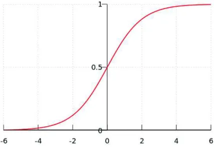
While speaking of parameters it is fitting to introduce the activation functions that are being used in practice. The unit step function mentioned above is not used in practice due to the fact that a small change in input can lead to a big change in output (0 to 1), an unwanted property since a continuous change in the output is preferable. [5] The sigmoid function (see figure 2.4) and the hyperbolic tangent function, smoother versions of the unit step function, have been used in practice but the activation function of choice today is the rectified linear unit function (ReLU), which is defined by returning only positive values, and variants of that function (see figure 2.5). [4] The output layer, or the classification layer, uses the softmax

(19)

Figure 2.3: A (simple) artificial neural network. Author: Michael Nielsen

Source: http://neuralnetworksanddeeplearning.com/chap1.html#the_architecture_of_ neural_networks

License: cbn

function, which outputs a probability distribution over all the categories. More informally the softmax function outputs the most likely category, the classification that the network found most probable.

To train a neural network we need some other kind of measure of how big the current error is outside of the training error, some kind of measure of how well off the weights and biases in the network are as whole. To solve this a cost or objective function is introduced, a function that measures the total current error. The two important properties such an objective function must have is that it is non-negative for all inputs, and that it is zero or close to zero if the error is small. [5] The direct goal of the training is thus to minimize the objective function. A simple approach here would be to choose the mean squared error as the cost to minimize, but in practice the cross entropy function is used instead due to a intrinsically better performance. [5]

Neural networks can contain millions, tens of millions and even billions of parameters and there is no feasible way to find the minimum with methods from ordinary calculus. Instead

(20)

Figure 2.4: Plot of the sigmoid function.

a algorithm called gradient descent, more precisely stochastic gradient descent, is used to minimize the objective function. [5] The method uses the gradient or derivative in a random starting point to find the current "slope" of the objective function, and decreases the value of the objective function with a fixed multiple of the absolute value of the gradient, which in more informal terms means that the algorithm moved down the "slope" a fixed amount towards the minimum. Applying gradient descent to a neural network means that each weight and each bias in the network is adjusted with a fixed multiple of the partial derivative of the objective function with regards to that specific weight or bias during each pass of the algorithm. The fixed multiples mentioned so far are multiplied with the learning rate, a hyperparameter of the network that can be tuned to boost performance. [5] Calculating the gradient over the whole training set would take too much time and isn’t used in practice. Instead the gradient is calculated for a randomly chosen subset of the training set, a so called minibatch, and used to update the network. This process is repeated for each minibatch in the training set until all minibatches have been processed. The time taken to process the entire training set is called an epoch, and training sessions are usually defined by the number of epochs. The fact that the training set is shuffled also explains the full name of the algorithm, stochastic gradient descent. [5]

(21)

Figure 2.5: Plot of the rectified linear unit (ReLU) function.

Even though stochastic gradient descent, as described above, is an algorithmic solution to a mathematically unsolvable problem it still needs further work to be useful in practice. Once again, neural networks have a huge amount of parameters and computing each partial deriva-tive of the objecderiva-tive function as in the naive implementation above is numerically unfeasible. The solution to the problem that makes stochastic gradient descent useful in practice is back-propagation, an algorithm that, simply put, calculates the error of one layer based upon the error of the preceding layer and updates its parameters accordingly. [5] The name of the al-gorithm comes from that property, that the error, and the correction of the error, propagates backwards through the entire network from the output layer and backwards. The elegance of the algorithm is that it mirrors the path the activations took forward in the network and car-ries roughly the same computational cost. As a final note on gradient descent there are more advanced variants in use today that builds upon the standard version with backpropagation, variants that adds additional elements such as dynamic learning rates and other tweaks. [4] Explaining those algorithms in detail are outside of the scope of this report, but it is worth mentioning that they exist.

(22)

As mentioned in the previous section there are inbuilt challenges connected to the machine learning process, and neural networks are no exception. The two problems that will be explored here are overfitting in the case of neural networks and the unstable gradient problem, a problem specific to the stochastic gradient descent algorithm applied to the training of neural networks. [5] Overfitting in this context is remedied by methods such as gathering more and better data, something that has been mentioned earlier in this chapter, and regularization. It has been mentioned in the former section, but it is worth repeating that regularization can be described as limiting the amount of functions the machine learning algorithm can generate. In the case of neural networks there are many kinds of regularization but the discussion here will restrict itself to these following methods: L1 regularization, L2 regularization, dropout and data augmentation. [5]

L1 and L2 regularization are two variants of the same theme and are built upon adding an extra term to the cost function, a term consisting of an weighted average of the sum of all the weights in the network. [5] The difference between the two lies in that the sum is of the absolute values of the weights in the former case and of the squares of the weights in the latter case. The reason why this term is added is to penalize networks with too large weights, a penalty whose effect, informally stated, is to make the network generalize better by forcing it to choose less complex functions linking input to output. [5] Dropout is a technique that is based upon dropping a random number of neurons in the hidden layers during each round of minibatches with a final adjustment of the weights in the end of a training run. The intended effect is, as with L1 and L2, to enforce better generalization. The last method, data augmentation, is built upon artificially expanding the available data by introducing random changes in the examples, e.g flipping an image horizontally, shifting it slightly in a direction or rotating it slightly. [5] Since the best cure for overfitting is more data this technique works in that direction to make the network generalize better.

The unstable gradient problem occurs due to the fact that the gradient, or the parameters’ rate of change, in a layer is a product of the rate change of all the layers before it. [5] This

(23)

can cause the rate of change to vanish entirely, the vanishing gradient problem, or go up drastically, the exploding gradient problem. The unwanted effects accumulate more rapidly the earlier in the network the layer in question is. This problem was, historically at least, a major hindrance to training networks beyond a certain depth. Luckily the problem seems to have been partially solved, partly due to the fact that the aforementioned rectified linear function and variants thereof have become the standard activation functions. A major cause of the problem was the use of saturating activation functions like the sigmoid and hyperbolic tangent functions, saturating in this context meaning the rate of change or derivative of the function goes to zero as the input becomes too large of a positive or negative number. [5] In contrast the ReLU function has a derivative that is either 0 or 1, which means that it does not saturate in its positive region and always propagate the gradient backwards. There have been other breakthroughs in this area, breakthroughs that will be discussed later.

During this exposition the terms neural networks and feedforward neural networks have been used synonymously, which is not surprising since it is the latter that has been discussed and explained during the majority of this chapter. The terms are not entirely synonymous though, since there are neural networks with loops and feedback connections. That subclass of neural networks is called recurrent neural networks, and makes use of more complex layers than the ones mentioned so far, layers such as long short-term memory units (LSTMs). [4] How recurrent neural networks work in detail is outside the scope of this report, but they are important and worth mentioning due to the fact that they are behind some of the latest breakthroughs in text and speech processing. There are other kinds of neural networks, but the focus of this work lies upon feedforward neural networks and their derivatives.

2.2.2 Convolutional Neural Networks

One of the weaknesses of an ordinary feedforward neural network with fully connected layers is that it has no prior inbuilt assumption about the data it is supposed to learn from. It is agnostic about the structure of the data and treats all data the same. [5] This can easily

(24)

become a problem partly due to the resulting redundant parameters, partly due to the size of the resulting redundancy since a neural network can, as mentioned several times before, grow very large. It is also counterintuitive to use this approach in the case of, for example, data consisting of images since it would mean that the spatial structure of the image would be ignored and the training would begin with the assumption that all pixels are equally related. [5] Another approach is clearly needed, which is why this sub-chapter deals with a special kind of feedforward neural networks, convolutional neural networks. Convolutional neural networks are designed with certain assumptions about the data, assumptions that fit image data but also other data with a similar internal structure.

The most fundamental operations of convolutional neural networks is, perhaps not surprisingly, convolutions. The concept of convolutions in the context of neural networks begins with the idea of layers consisting of neurons with a local receptive field, i.e. neurons which are connected to a limited region of the input data and not the whole. [5] In the case of image data that means that each neuron is connected to only a limited region of pixels, e.g. a square of 3 x 3 pixels in the upper left corner of an image. The receptive fields of the neurons are also overlapping to a certain degree, in that (continuing the example from the sentence before) two adjacent neurons have receptive fields that are shifted by one or more pixels horizontally or vertically in relation to each other. One can visualize a sliding window of a given size, sliding from left to right and top to bottom (the data can be assumed to have a two-dimensional structure from now on), connecting the output of the window in each pass to a neuron. The result will be a two-dimensional structure of its own, a map or image of the activations from each neuron. The "sliding window" in this context is more properly called a kernel, a set of weights and a bias. That means that each neuron in such a layer or map shares the same parameters and thus could be said to learn the same feature, which leads to the proper name for such structures, feature maps. The operation described above, applying a kernel to an input map and generating a feature map, is a convolution. [5] The usage of convolutions is, intuitively, highly fitting for highly spatially correlated data since one can argue that, for example, two pixels in and around the eye in picture of a face has a more meaningful relationship than two

(25)

pixels chosen at random from the picture.

Figure 2.6: A hidden layer of neurons with locally receptive fields. Author: Michael Nielsen

Source: http://neuralnetworksanddeeplearning.com/chap6.html#introducing_ convolutional_networks

License: cbn

The convolutional layers in convolutional neural networks consists of multiple, stacked feature maps with associated neurons. This is also why the kernels associated with the feature maps are also called filters or channels. [6] Convolutional layers can also be stacked upon other convolutional layers, which in more informal terms can be described as building feature maps upon feature maps or learning higher-level features. One other important aspect of convolu-tional neural networks is that the parameter sharing involved decreases the absolute number of parameters needed, in addition to a major relative decrease of parameters in comparison to a network using only fully connected layers to do the same task. In general, the formula for the number of parameters in a convolutional layer performing two dimensional convolutions is (M ∗ X ∗ Y + 1) ∗ N, where M is the number of feature maps in the input (counting the red-green-blue channels in colored images), X and Y the height and the width of the convolution (3 x 3, 5 x 5, etc.) and N the number of feature maps in the output, the one added to account for the bias. [7] The two final aspects of convolutions to be discussed in this section are stride and padding. In the previous paragraph it was implicit that the size of the step, or stride, during the convolution was one, but higher strides can be used as well. Padding of the input

(26)

is used to preserve the spatial resolution during the convolution, since it shrinks without it by a constant factor in both dimensions depending on the size of the convolution. [5]

Another kind of important layer in convolutional neural networks are pooling layers which apply the pooling operation. Pooling in general consists of transforming feature maps to smaller, more aggregated feature maps. [5] The most common kind of pooling is max-pooling, which takes non-overlapping regions of a given size and outputs the largest activation in that region, e.g. splitting the input map into sections of size 2 x 2, choosing the maximum value and creating an output map consisting of those values, but only a fourth of the original size. A pooling layer thus pools the input from a preceding convolutional layer, preserving the number of feature maps. The rationale behind pooling is to shrink the spatial dimensionality in the network while preserving spatial information, using the strong correlation between data points that are close to each other. [4] As with convolutions, pooling layers can use stride to achieve even greater aggregation.

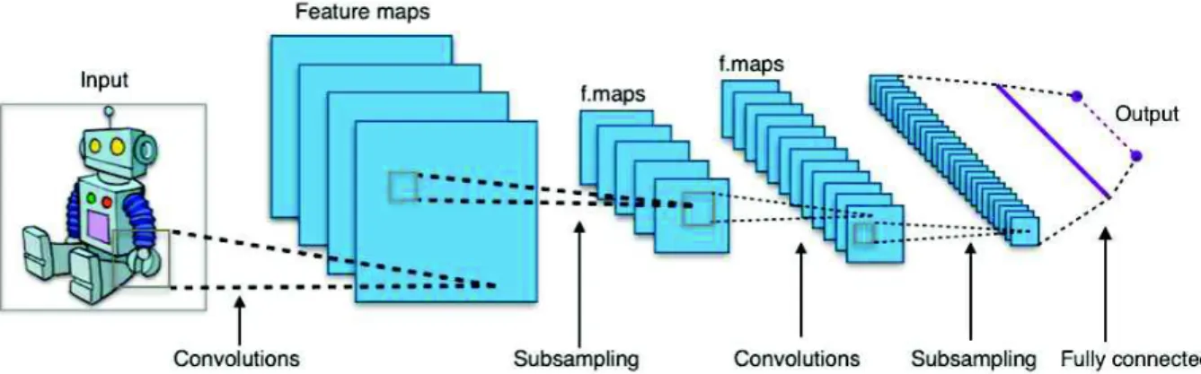
With pooling layers introduced, the structure of a convolutional neural network can be made clearer. The overarching goal of a convolutional neural network is to transform the spatial representation of the input to a representation rich in features, a large feature space from which to classify. The basic structure of a convolutional neural network is thus convolutional layers alternated as fitting with pooling layers, combined with using the techniques discussed in the previous section, and usually a couple of fully connected layers with a classifier at the end. [5] This structure has been around for years, at least since Yann LeCuns LeNet5 architecture in 1998 [8], but the same ideas are still useful today. It merits to mention that the basic approach still works, especially since the research around convolutional neural networks is intense and that many major breakthroughs have been made and are being made, especially in the areas of image classification and object detection.

(27)

Figure 2.7: A simple convolutional neural network. Author: Aphex34

Source: https://commons.wikimedia.org/wiki/File:Typical_cnn.png License: cba

2.2.3 Neural Network Designs and Architectures

In this section some of the more significant neural network designs and architectures, more particularly those of convolutional neural networks, will be introduced in appropriate detail. The common task all of the following architectures are geared towards is image classification, to be able to classify images as correctly as possible into a number of predetermined categories.

The first major breakthrough after the LeNet5 model mentioned in the previous section was Alex Krizhevsky’s AlexNet in 2012 [9], a contribution to the ImageNet competition. ImageNet is a database consisting of a million images sorted into a thousand categories being used for research into image recognition and object detection. [10] AlexNet built upon the approach of LeNet5, used rectified linear units and ran on two GPU:s. [9] This approach was refined further with the VGG (Visual Geometry Group) networks, networks with a much greater depth and accuracy. [11] The main innovation was the use of smaller convolutions of size 3x3 and 5x5 instead of the much larger convolutions used in AlexNet, and the stacking of layers using these smaller convolutions upon each other. [6] The networks grew quite large, however, and the training had to be done in parts due to the sheer difficulty of it. [6] The run-time performance

(28)

of the VGG networks during inference, or classification after training is done, was also quite costly. [12]

The approach mentioned above has, as mentioned, some obvious drawbacks, especially regard-ing the computational burden of trainregard-ing and servregard-ing the model. A research team at Google took another approach with those considerations in mind, an approach that resulted in the 2014 winner of the ImageNet competition, GoogleNet, a network design based upon Inception modules and the first network to use the Inception architecture. [13] The basic idea behind an Inception module is to have layers working on input in parallel, both convolutional layers and pooling layers, layers with different sizes of kernels, and then concatenating the outputs into a single layer. GoogleNet began with an ordinary stack of layers as those in the aforementioned AlexNet and VGG models, a large middle part of Inception modules stacked upon each other and finally a global averaging layer with a softmax classifier, the last part inspired by the Network In Network paper. [14] Another important aspect of the Inception architecture is the use of 1x1 convolutions. 1x1 convolutions serves two useful purposes in convolutional neural networks; they can be used to cheaply, computationally speaking, add nonlinearity via extra activations and to reduce the number of features in the outgoing layer cheaply. [6] These convo-lutions are used to build so called bottleneck layers, constructs consisting of a layer using 1x1 convolutions to downsample the outgoing features by usually a factor of four, a second layer using a larger kernel on the smaller number of features and a final layer of 1x1 convolutions to upsample the features again. These bottlenecks can reduce the numbers of computations needed by nearly a factor of ten. [6] The combination of bottlenecks and Inception modules has led to the success of the architecture and the following network designs, Inception V2 [15] and V3 [16]. The Inception networks has, in comparison to the VGG networks and the approach behind them, increased the accuracy in the ImageNet Challenge while decreasing the number of parameters and the number of operations significantly. [6] [12]

The final approach to be introduced here is that of the Microsoft team behind ResNet, the winner of the ImageNet competition 2015 and an architectural approach that achieved an

(29)

Figure 2.8: An Inception V1 module. Recreation of an image from: [6]

unprecedented network depth by using a new technique: residual blocks consisting of several layers, and networks consisting of those blocks, residual neural networks. [17] The basic idea of residual blocks is to run the input through two or more layers and then, crucially, adding the initial input to the output of the second layer, neuron for neuron, and applying the activation function to get the output of the block. The block can be said to consist of an residual connection, the layers the input is run through, and a skip connection, the bypassing of the initial input. [18] The residual connection is usually a bottleneck layer, and the skip connection is usually only the input, but other variants exist, primarily to cut down the spatial dimensionality. [17] The team behind ResNet managed to use the residual blocks to design and train a convolutional neural network with over a thousand layers, a record in deep learning. [6]

(30)

Figure 2.9: A residual block with an ordinary skip connection. Recreation of an image from: [6]

Research concerning new designs and new architectural approaches is being published con-tinuously and rapidly, and we have not prioritized presenting the most current designs here. What has been presented here is some of the more significant approaches in later years. There are of course a plethora of other interesting designs that could be mentioned, such as a design with the same performance as AlexNet but with 50 times less parameters [19], a design with the alternating pooling layers replaced with convolutional layers [20] and a design which uses a variant of ResNet to achieve state of the art performance on certain problems. [21].

2.3 Deep Learning Frameworks

This chapter introduces the reader to the deep learning frameworks used in this study, as well as some other other deep learning frameworks, but firstly: a short introduction to the

(31)

purposes and functions of deep learning frameworks in general.

The algorithms and functions used in machine learning, and especially deep learning, involves a lot of mathematics; it can therefore be difficult and time consuming to implement the neural network from the ground up. Deep learning frameworks provide a high level API in order to make the implementation of neural networks simpler and more efficient. The frameworks make the implementation simpler and more efficient by abstracting away the underlying mathematics and by providing premade modules and code. By abstracting away the mathematical implementation the frameworks remove the requirement for the programmer to have an extensive mathematical background, thus making deep learning easier to work with and more available.

2.3.1 The Frameworks Used in This Study

The frameworks used in this study are: Google TensorFlow [22] and The Microsoft Cognitive Toolkit (CNTK) [23]. A third party API called Keras was used for TensorFlow. Keras provides a higher level, and more user friendly API, and is capable of running both TensorFlow and another deep learning framework called Theano [24], as backend. [25] There are also plans to develop a CNTK Keras backend. [26]

Google TensorFlow is an open source deep learning and machine learning framework developed by Google and was initially released on November 9, 2015; the stable version was released on February 15, 2017. TensorFlow is written i C++ and Python, and provides interfaces for Python, C++, Java, Haskell, and Go. [27] TensorFlow was originally developed for the purpose of conducting machine learning and deep neural networks research. TensorFlow supports computation over multiple GPUs or CPUs, both locally and distributed. [22] [28]

Microsoft CNTK is an open source deep learning framework developed by Microsoft and was initially released January 25, 2016; and has, as of this writing, not had a stable re-lease. CNTK is written in C++ [29], and provides interfaces for Python, C++, C# [30], and Microsoft’s own scripting language for deep learning: BrainScript. [31] CNTK was initially

(32)

developed for Microsoft themselves for fast training on large datasets. [32] Many of Microsoft’s own products uses CNTK, e.g. Cortana, Bing, and Skype. [23] CNTK supports computation on CPU [33] and multiple GPUs, both locally and distributed [34], as well as training and hosting models on Azure. [35] [36]

There are a lot of other frameworks to choose from including: Theano [24], Torch [37], Caffe [38], and Deeplearning4j [39]

2.4 Summary

In this chapter the project has been introduced as well as the rationale behind it and its scope, to compare and evaluate deep learning frameworks. The general concepts behind machine learning, the goal of training a program to generalize well, the difference between optimization and machine learning as well as some of the challenges have been introduced to an appropriate degree. The machine learning algorithm this project is based upon, neu-ral networks, and a major derivative, convolutional neuneu-ral networks, have been introduced, explained and illustrated. Some of the more noteworthy designs and architectural choices have also been covered. The frameworks that we will be using in the project have also been introduced as well as other deep learning frameworks.

The project as a whole is partly based upon evaluating two deep learning frameworks, Google TensorFlow and Microsoft CNTK, and partly based upon learning about and applying ma-chine learning in the form of neural networks, more specifically convolutional neural networks. Neural networks is one of the most prominent machine learning algorithms in use today, es-pecially in the context of training networks with many layers, deep learning. The focus lies in particular upon convolutional neural networks, a variant of neural networks adapted for data with prominent spatial relations, the type of data related to problems as image classification and object detection. The designs of and the architectural approaches to convolutional neural networks have been rapidly developing in later years, and the results have been

(33)

groundbreak-ing. The tools to implement deep learning have also been rapidly developing in later years, and there are a lot of frameworks and libraries to choose from.

(34)

3 Project Design

The purpose of this project is to evaluate two frameworks for machine learning: Microsoft CNTK and Google TensorFlow. This chapter will present an overview of the different parts of the evaluation and the evaluation method used for the different parts. Chapter 3.1 covers the installation and the system requirements of the two frameworks and their dependencies; as well as the frameworks’ support of programming languages. Chapter 3.2 covers the frameworks’ features, functionalities and documentation; as well as their support for third-party API:s. Chapter 3.3 covers the frameworks’ performance using two widely used data sets for bench-marking machine learning models; Mixed National Institute of Standards and Technology [1] dataset of handwritten numbers (MNIST) and Canadian Institute for Advanced Research’s dataset of tiny images in color (CIFAR-10) [2]. Chapter 3.4 presents the design of a custom built image classifier; its development process and performance will be used in the evaluation of the frameworks’ performance and user friendliness. At the end of the chapter a summary is provided.

3.1 Installation and System Requirements

In this part of the evaluation the system requirements of Microsoft CNTK and Google Tensor-Flow will be compared, including their dependencies. In the evaluation the following is taken into consideration: ease and speed of installation, system requirements, software and hard-ware support, and programming language support. Additionally, the system requirements to be able to perform the necessary calculations on GPU instead of CPU, as well as the ease of setting that up, will be evaluated. A development environment with the necessary tools will be set up as well.

3.2 Features, Functionalities and Documentation

In this part of the project CNTK:s and TensorFlow’s features, functionalities, and documen-tation will be evaluated and set against each other. The evaluation will begin by studying the frameworks’ documentation to ascertain the following: which machine learning algorithms

(35)

the frameworks provide, how intuitive the frameworks’ API:s are; how well documented the frameworks are, and other features and functionalities the frameworks provide; as well as their support for third party API:s. The results of the evaluation will be used in comparing the frameworks.

3.3 Benchmarking Tests

In a comparative study of software frameworks such as TensorFlow and CNTK one may make a distinction between the softer criteria, e.g. personal experiences and perceived ease of use, from the harder criteria, e.g. numerical benchmarking data and the objective failure of a program developed with these frameworks as aid to perform a task in a given time span. The distinction is not always easy to make in practice, nor always relevant for the task at hand. Data must be interpreted and put into proper context and other subjective factors almost always come into play to muddy the picture. It is nonetheless, in our opinion, a fruitful approach to identify as many objective, or "hard", aspects of our study as possible, with results that mostly speak on their own.

The part of the project that is to be designed here is the laboratory environment where we to the best of our ability remove, or turn into constants, as many variables and parameters as possible in all aspects of the process, from the software to the hardware, in order to reliably benchmark the performance in terms of time taken, GPU/CPU usage, memory usage and other relevant factors. Part of that design consists of developing the same exact model, down to each individual layer and each parameter, in the API:s of both frameworks. Another part is making sure that the data sets in question are preprocessed identically in the pairs of models that are learning from them, and that the data sets in question are well chosen concerning quality and availability.

The datasets that will be used to benchmark the frameworks are the MNIST database of 70000 images, and the CIFAR-10 database of 60000 images. The MNIST database consists of 70000 black and white images of handwritten numbers, 0 to 9 and 28x28 pixels large, and the

(36)

task the corresponding model is supposed to learn is to classify the images into ten classes, one for each number. The CIFAR-10 database consists of 60000 images in color, 32x32 pixels large, and the task the corresponding model is supposed to learn is to classify the images into ten classes as follows: airplane, automobile, bird, cat, deer, dog, frog, horse, ship and truck.

A large part of the work in this chapter of the project will consist of learning to pick apart and redesigning existing models. Since the datasets mentioned above, MNIST and CIFAR-10, are common academic benchmarks for performance there already are examples shipped with the frameworks, examples that are ready to run with a single command. The substantial work that is to be done here is the refactoring of the examples, identifying what each part of the code does and rewriting each model until the architecture, the parameters and all other design factors are the same. The work that is to be done here is, firstly, to create two designs and, secondly, to implement each design in each of the two frameworks.

The final part; the actual benchmarking and gathering of measurement data, will be done with a combination of system monitoring tools to monitor GPU/CPU usage and memory usage. What tools to be used during the actual benchmarking will be decided during the implementation. The data that is the most important for the purpose of benchmarking are the following:

• The time it takes to finish a complete training run with a given model on a dataset.

• The GPU usage and, in special cases, the CPU usage in operations per second and in the percentage of the total capacity over time.

• The memory usage, again measured both in gigabytes and in the percentage of the total capacity over time.

The data above needs to be averaged over multiple training runs; e.g. five training runs per benchmarking session and model. Visualizing the data in the form of diagrams will be

(37)

necessary in due course, but the type of diagrams and the software that will be used for the drawing lies outside of the scope of the project design.

3.4 Implementing an Image Classifier

Since the project specification did not specify a concrete problem to solve; a problem first needs to be found and decided on. The problem needs to be not too complex, while still not being too trivial. We know that we want to implement some kind of image classifier; what kind of images however, and how specific the image classification; e.g. classifying different objects or more specifically classifying different types of the same object, that remains a part of the implementation. A sufficient amount of data of sufficient quality is also needed to be able to train and test the image classifier; what sufficient means in numerical terms and in practice; may fall on the implementation chapter as well.

The first task in this part of the project is therefore to find and look at different sources of data sets; decide on a problem of reasonable complexity, where a sufficient amount of data can be acquired for training and testing the image classifier. After that the data of course needs to be downloaded.

The second task is to begin implementing the image classifier. The image classifier will be implemented in both Microsoft CNTK and Google TensorFlow, using TensorFlow as back end with Keras, a third party API for deep learning, as front end. Keras is usable as front end to TensorFlow today, the process to add Keras to the TensorFlow core is ongoing as of this January [40] and will probably be able to use CNTK as back end at some point in the future as well [26]. All the different models of the image classifier in the different frameworks will be implemented and developed in the same programming language and development environment, to make the models more comparable. The programming language that will be used for the implementation is Python 3 [41] and the development environment that will be used is Microsoft Visual Studio 2015 Enterprise [42] with the Python Tools for Visual Studio plug-in [43] installed. In addition to using the same programming language and IDE

(38)

(Integrated Development Environment), we will also strive to make the models as similar as possible code wise; i.e. as similar as the frameworks allow; again, to make the models as comparable as possible.

The third and final task is to start training and testing the different models developed in the two frameworks, Microsoft CNTK and Google TensorFlow with Keras as front end. In the end the models development process, performance and their test accuracy will be used as part of the evaluation and comparison of the frameworks’ performance and user friendliness. In this part of the project, the more softer aspects of the frameworks are of more interest, since the frameworks’ raw performance will be tested in the benchmarking tests, see chapter 3.3. The more softer aspects that will be considered are: how intuitive the frameworks API:s are, ease of development, and speed of development. The previously mentioned criteria are of course of a more subjective nature, but we will strive to motivate our conclusions with as well grounded arguments as possible. In addition to the comparative aspect described above this part of the projects also contains an exploratory aspect in the form of designing and implementing the models themselves, choosing and evaluating different techniques and analyzing the performance of the models.

3.5 Summary

In this chapter the general design of the project has been laid out. The project as a whole is a larger evaluation and comparison of the two machine learning frameworks Microsoft CNTK and Google TensorFlow. In the evaluation both softer and harder aspects are considered, such as: ease of installation, system requirements, programming language support, user friendli-ness; performance, test accuracy, as well as ease and speed of development. The frameworks’ documentation will be studied and evaluated.

As a part of the evaluation, a number of tests will be performed in order to evaluate the more harder aspects, such as the frameworks’ performance and test accuracy. These tests include training and testing models developed in each framework on two well known machine

(39)

learning benchmarking tests: MNIST and CIFAR-10. Finally, a custom image classifier will be developed in each framework in order for the authors to get a first hand grip of the frameworks’ user friendliness, the ease and speed of development in each framework and the process of designing the models and evaluating their performance.

(40)

4 Project Implementation

In this chapter the actual implementation of the project’s parts described in chapter 3 will be described. The sub-chapters are mirrored after chapter 3’s ditto, for ease of reference.

4.1 Installation and System Requirements

In order to gather the necessary information to evaluate the system requirements, software and hardware support, and programming language support; TensorFlow’s and Keras’, and CNTKs documentation was studied. In order to evaluate the ease and speed of installation, the frameworks were downloaded and installed. This is the more subjective part of this part of the evaluation. The aspects that the conclusions are based on are: the amount of steps required to be able to use the framework, and the perceived ease to follow the aforementioned steps. Written below are the steps the authors used to install each respective framework.

Firstly, the development environment needed to be set up. Since the development is to be done in Python, Python 3.5.3 was downloaded and installed from Python’s homepage https:// www.python.org/. The IDE used was Microsoft Visual Studio 2015 Enterprise [42], which was already installed on the computers used in this study. To be able to use Python in Visual Studio the Python Tools for Visual Studio (PTVS) extension [43] needed to be installed. To install PTVS, the Visual Studio installation was modified through the Windows Control Panel with the added PTVS extension.

Google TensorFlow was downloaded and installed through Visual Studio, with PTVS, using the built-in tool pip. To be able to use the GPU, TensorFlow’s GPU version 0.12.1 was installed, pip handles and installs all python related dependencies. When using TensorFlow’s GPU version two additional downloads were required: the NVIDIA CUDA Toolkit 8.0, and the NVIDIA cuDNN v5.1 (CUDA Deep Neural Network) library, which were downloaded from https://developer.nvidia.com/cuda-downloads, and https://developer.nvidia.com/cudnn respectively. The cuDNN’s dll-file was placed in the CUDA-folder created after installing the CUDA Toolkit.

(41)

Keras was downloaded and installed through Visual Studio, with PTVS, using the built-in tool pip. The version installed was 1.2.2. Pip handles and installs all python related dependencies, however the scipy and numpy versions installed through pip were wrong, and needed to be downloaded and installed manually. The correct versions of scipy and numpy needed by Keras were downloaded from this site: http://www.lfd.uci.edu/~gohlke/pythonlibs/. The downloaded whl-files of the correct versions of scipy and numpy were installed using pip through the Windows Command Prompt.

Microsoft CNTK was downloaded from https://github.com/Microsoft/CNTK/wiki/Setup-Windows-Binary-and installed manually. The version installed was the Beta GPU version 10 using the binary

installation with scripts. Installation using pip was not available at the time of installation, but has since been added. The CNTK binary installation with scripts includes all dependen-cies, including NVIDIA CUDA Toolkit 8.0 and NVIDIA cuDNN v5.1, which were installed along with CNTK itself; the installation also included an Anaconda environment [44], in which CNTK is supposed to run.

4.2 Features, Functionalities and Documentation

The work that was done to compare the two frameworks, CNTK and TensorFlow, according to the criteria in the corresponding sub-chapter of the project design, consisted of an in-depth reading of the documentation (in the case of TensorFlow primarily that of Keras’) to understand the workings of the frameworks, notes taken during the development and testing process and a final evaluation of the gathered information based upon a refined set of criteria. The following four criteria were chosen: features and functionalities, quantity and quality of documentation, extensibility and interoperability and cognitive load. The criteria the authors chose and the evaluation process will be elaborated upon below.

(42)

evaluation process followed from the rationale of the project. Features and functionalities in this context means, more precisely, the tools available in the frameworks to implement neural networks and deep learning. Another aspect evaluated in relation to this criteria was also how the tools are implemented in the form of classes, methods and functions, but not in specific detail.

Since proper documentation is a necessary tool in the development process the frameworks were evaluated on the quantity and quality of the documentation available. The steps needed to find the desired information in the documentation, the amount of information available, the ease of access to tutorials, the frequency of updates to the documentation and the ease of navigating the source code were all aspects of the documentation that the frameworks were evaluated by in the process. The amount of missing and incomplete information in the documentation of the frameworks were also considered in the context of this criteria.

The extensibility and interoperability of the frameworks was not a criteria that was tested directly in either the benchmarking process, nor in the process to design and implement the image classifier. It was, however, found prudent to include it as a criteria since the details of actually deploying the model in application is important. The aspects that were evaluated here were how the deployment process might work and how the frameworks integrate with other languages, libraries and frameworks. The information acquired here were taken from the documentation of the frameworks since, once again, the criteria did not come up in the other work done within the project.

Cognitive load is a concept originated in cognitive psychology, referring to the total amount of mental effort being used in the working memory. [45] In the context of this report the term is referring to the amount of mental effort it took to learn, use and develop in the frameworks. The motivation behind the criteria is that it in general, all other things being equal, is better with a framework that is easy to use than a framework that demands a lot from the developer. Other aspects grouped under this criteria that was used during the evaluation

(43)

process are how much the frameworks conformed to the principle of least astonishment [46], how much boilerplate that was required and how well the implementations in the frameworks conformed to the literature.

4.3 Benchmarking Tests

The System used in this part of the project Operating system: 64-bit Windows 8.1

CPU: Intel Core i7-4800MQ @ 2.80GHz

RAM: 32GB

GPU: NVIDIA Quadro K2100M 2GB

Other: TensorFlow-gpu 1.0.1, Keras 2.0.2, CNTK 2.0.beta15.0, Numpy 1.12.1 + mkl, Scipy 0.19.0, PyYaml 3.12, NVIDIA graphics driver version 376.51, NVIDIA CUDA Toolkit 8.0, NVIDIA cuDNN v5.1

We had updated TensorFlow, Keras, and CNTK since we first installed them before run-ning the benchmarking tests. The frameworks’ versions during this part of the project were: TensorFlow GPU 1.0.1, Keras 2.0.2, CNTK GPU beta 15. Both Keras and CNTK provided premade code examples for training neural networks on the MNIST and CIFAR-10 datasets. We used the given code examples for each respective dataset to get started and tried to make them as similar as possible in both frameworks, given our knowledge of the frameworks’ under-lying implementation and the theoretical background. We started working with the given code examples for the MNIST dataset, followed by CIFAR-10s ditto once the MNIST ones were complete. We followed the same working procedure during the implementation of the neural networks for both MNIST and CIFAR-10. The working procedure was as follows: studying the code and the documentation to understand each step in the code, finding where the code examples differ, and studying the documentation to find a substitute solution which can be made as similar as possible in both frameworks.

(44)

The prime factor in this part of the project is not the models’ testing accuracy but evaluating the frameworks’ performance, especially training time. The system was monitored during the training process using ASUS GPU Tweak. The training time for each epoch was printed to standard output using built-in functions in the frameworks. We ran five separate training and testing runs for each model in each framework, totaling four models and twenty runs. The models trained on MNIST went through twenty training epochs in each run. The models trained on CIFAR-10 went through forty training epochs in each run.

4.4 Implementing an Image Classifier The System used in this part of the project Operating system: 64-bit Windows 10

CPU: Intel Core i7-4790k @ 4.4GHz

RAM: 16GB

GPU: NVIDIA GTX 970 4GB

Other: TensorFlow-gpu 1.1.0, Keras 2.0.3, Numpy 1.12.1 + mkl, Scipy 0.19.0, PyYaml 3.12, Matplotlib 2.0.0, NVIDIA graphics driver version 376.51, NVIDIA CUDA Toolkit 8.0, NVIDIA cuDNN v5.1

The main difference between the approach set out in the corresponding chapter of the project design and the work that was actually done is that the resulting image classifier was written in Keras, with TensorFlow as backend, but not in CNTK. The problems encountered while working with CNTK, as outlined in chapter 5.2, combined with the time constraints made it impossible to implement the classifier in both frameworks. This means that the comparative aspect in this part of the project had to be left out, with only the exploratory aspect left. The rest of the process followed the project design and consisted of two parts, finding and deciding upon a dataset and then implementing the image classifier, through coding and training the resulting network.

(45)

The dataset we decided upon using was a variant of the CIFAR dataset, the same dataset we used during the benchmarking process as documented in the previous chapter, but with a different labeling. The CIFAR-100 dataset has 100 classes, classes that are grouped into 20 superclasses. Each example in the dataset is labeled with both the class it belongs and the superclass it belongs to. The motivation behind the choice of using CIFAR-100 as the dataset to train an image classifier on can be divided into several reasons. The first and foremost reason is that the dataset is widely used in research and development, which means that the quality of the data was not an unknown and could be counted upon. Another reason is that the use of an existing, easily available dataset saved considerable time and effort by eliminating the work that it takes to gather, prepare och preprocess the data needed to train the image classifier. The third and final reason is that the design and implementation of the network could make use of the work done in the benchmarking part of the project, since related problems had been worked through and tested there.

The network was designed and implemented using a variety of different techniques as follows: exponential linear units, residual blocks, global average pooling, dropout and data augmenta-tion. The choice of activation function, the exponential linear unit (ELU) function, is a variant of the ReLU function that allows a small gradient to flow through if the input is negative, a property of the function that is purported to have a normalizing effect on output by making the activations closer to the mean. [47] The residual blocks that we used as the main tool in the design have been introduced in chapter 2.2, and two variants were used, the first consist-ing of an unaltered skip connection and an ordinary bottleneck layer and a second one usconsist-ing 1x1 convolutions with stride 2 to shrink the spatial dimensionality. The reason why residual blocks were chosen is partly due to the impressive results achieved by the use of networks using residual connections, partly due to the relative ease of understanding och implementing them in the classifier. Alternatives such as the Inception architecture were found both too complex and too inflexible in terms of flexibility and scalability.