A study of calculation models for fatigue life prediction

(1)

A study of calculation models for

fatigue life prediction

A thesis accomplished together with GKN Aerospace

En undersökning av beräkningsmodeller för utmattningslivslängd

Rebecca Aikio Englund

Faculty: Health, Science & Technology

Subject: Bachelor of science in mechanical engineering Points: 15 HP

Supervisor: Henrik Jackman Examinator: Anders Gåård Date: 2018-06-12

(2)

Abstract

GKN Aerospace in Trollhättan don’t use the latest ANSYS version and need to upgrade their life analysis models. The aim with this thesis is to do a study of the new models and

investigate the times required for the calculations. A flight mission were chosen and this mission together with different life analysis models were run in the GKN in house program Life Analysis System. The results were analyzed and depending on the results additional runs were made or the problem were sent to the life management group at GKN Aerospace. Strain levels versus time were also plotted for the runs with the new models to get a perception where any problems occurs. The results from the model 4.10.149 had no variations between equal runs for the high pressure turbine and the low pressure turbine but there was a variation between the results when equal runs was made with the high pressure compressor. The results from model 4.10.157 and 4.10.124 and 4.10.160 and 4.10.173 had variations in the fatigue life for equal runs. The variations can depend on that the calculations converges to different solutions, the reason for this can depend on the non-linear contact elements. The variation in the results between equal runs occurs when the model uses two or more cores. The time required for the calculation becomes faster with the use of more cores. The longest duration had model 4.10.173 because of the many requirements for the calculations in this model. The problem with the variation in the results is sent to ANSYS.

(3)

Sammanfattning

GKN Aerospace i Trollhättan använder inte den senaste versionen av ANSYS och behöver uppdatera deras livsanalys beräkningsmodeller. Syftet med denna rapport är att göra en undersökning av de nya modellerna och av tiderna som krävs för beräkningarna. Ett flygpass valdes slumpmässigt och dessa flygpass tillsammans med olika beräkningsmodeller testades i GKN´s egna program Life Tracking System (LTS). Resultaten analyserades och fler tester utfördes eller så var eventuella problem skickade till hållfasthetsavdelningen på GKN Aerospace. Töjningen mot tid plottades även för de nya modellerna för att få en uppfattning av var eventuella problem inträffade. Resultaten från 4.10.149 var bra för högtrycksturbinen (HPT) och lågtrycksturbinen (LPT) men innehöll variation i resultaten då likadana test utfördes för högtryckskompressorn (HPC). Resultaten från modell 4.10.157, 4.10.124, 4.10.160 och 4.10.173 innehöll också variationer i utmattningslivslängd mellan likadana tester. Dessa variationer kan bero på att beräkningarna konvergerar till olika lösningar som kan bero på att problemet innehåller olinjära kontaktelement. Detta händer då modellerna använder fler än en kärna för sina beräkningar. Den modell som krävde längst tid för sina beräkningar var modell 4.10.173 på grund av många krav på beräkningarna med denna modell. Problemet med variationer har skickats till ANSYS för hjälp.

(4)

3. Methods ... 12 3.1 Old models ... 12 3.2 New Models ... 12 3.2.2 Strain levels ... 13 4. Results ... 14 4.1 Old Models ... 14 4.1.1 Model 4.10.149 ... 14 4.1.2 Model 4.10.167... 15 4.1.3 Model 4.10.157... 16 4.2 New models ... 18 4.2.1 Model 4.10.124... 18 4.2.2 Model 4.10.160... 21 4.2.2.1 Strain Analysis ... 23 4.2.3 Model 4.10.173... 24 4.3 Time aspect ... 25

(5)

5 Discussion ... 27 5.1 Old models ... 27 5.2 New models ... 27 5.3 Time aspect ... 28 5.4 Method ... 29 5.5 Future work ... 29 6 Conclusions ... 30 7 Acknowledgements ... 31 8 References ... 32 APPENDIX 1. Runs from model 4.10.149

APPENDIX 2. Runs from Model 4.10.167 APPENDIX 3. Runs from model 4.10.157 APPENDIX 4. Runs from model 4.10.124 APPENDIX 5. Runs from model 4.10.160 APPENDIX 6. Runs from model 4.10.173

(6)

1

1. Introduction

This bachelor thesis will provide information about the GKN Aerospace in house program called Life Tracking System. The report will obtain an analysis about life analysis calculating models and a new computer cluster at GKN Aerospace in Trollhättan. The supervisor at GKN Aerospace for this study is Magnus Andersson.

1.1 Background

Calculating life limits and life consumptions for different engines is an important way to maintain safety and reduce maintenance costs. It’s in GKN Aerospace interests to do

improvements through more accurate life analysis models and less uncertainties, in this way the engines may be used for longer times which reduces the costs or the engine may be used for shorter times which maintain flight safety. In which way there’s a positive outcome but there’s also a big responsibility to calculate this type of calculations and a lot of validations that insures that the calculations works correctly needs to be done before the calculations can be used in the real life. GKN Aerospace Sweden AB has developed a system for more precise life consumption calculation called Life Tracking System (LTS).

GKN Aerospace has a life management group who works with Life Analysis System (LAS) and LTS. They don’t use the latest version in ANSYS and has a plan to upgrade the ANSYS version this year. ANSYS is an engineering simulation software. With a new ANSYS version they need to upgrade the models used for their life calculations. In the past there has been difficulties with upgrading the models, the problem has been variations for the fatigue life when a flight mission is tested several times even though the tests are equal. They will also upgrade their computer cluster in hope that it will shorten the calculation times. Before the new models and cluster can be used in production they need to be tested.

1.1.2 GKN AEROSPACE

The GKN group has over 59000 employees across 30 countries. GKN Aerospace Sweden is a part of GKN group and has itself over 2400 employees across 4 countries, Sweden

(Trollhättan), Norway (Kongsberg), Mexico and the USA. The head office is placed in Trollhättan, Sweden. GKN Aerospace Sweden works with aeroengines, components to aeroengines and space rockets. They are also responsible for the maintenance of aircraft engines both commercial and military. They are specialized for about 10 advanced component in the civil aeroengines and these components is today located in 90% of all new bigger

(7)

2

passenger aircrafts. They have also been manufacturing and been responsible for the engines in the Swedish Air force since 1930. The Swedish air force JAS 39 Gripen can be seen in figure 1. [1-3]

Figure 1. The JAS 39 GRIPEN C/D. Permission to use picture by GKN Aerospace. [4]

1.2 Nomenclature

ELCF- Equivalent low cycle fatigue HPC- High pressure compressor HPT- High pressure turbine LAS- Life Analysis System LPT-Low pressure turbine LTS – Life Tracking System

RM12- Engine in the Gripen C/D fighter

1.3 Problem

The fatigue life calculations requires a lot of capacity from the computer like CPU-power, memory, disk and network speed and are also time consuming. Therefore, there is always a need to upgrade parts of the systems. In this work, tests with old and new models from the

(8)

3

GKN life management group will be compared, both results and times will be compared to look after improvements or any problems with the models. A new cluster at GKN Aerospace will also be investigated to see if the cluster gave improvements in the results and the times required for the calculations.

1.4 Aims and goal

The aims with this project are to do a study of different models used for calculating fatigue life and to investigate if updated models and the new cluster will perform the calculations faster.

The goal is to do a documentation of the study for different models used for calculating life consumptions and for a new computer cluster. A report will be provided about LTS and give an update about the work with the testing of models used in LTS and a new computer cluster.

1.5 Restrictions

Exact figures and results are not included in this public version of the thesis. APPENDIX 1-7 are not included in this public thesis. Neither is information about the specific flight mission used for this public thesis.

1.6 Delimitations

In this report will look at three different modules of the RM12 engine used for Gripen C/D fighter, the high pressure turbine (HPT), the low pressure turbine (LPT) and the high pressure compressor (HPC). These are critical modules in the RM12 engine. The priorities will be in the same order, HPT, LPT, HPC. This is because the project has a time limit.

(9)

4

2. Theory

2.1 RM12

GKN Aerospace is the original equipment manufacturer for the RM12 engine. GKN’s responsibility covers different areas in the RM12 engine used in all the Gripen C/D fighters such as the complete design, development, assembly, manufacturing, certification and technical support. The RM12 engine is used by air forces in Sweden, South Africa, Czech Republic, Hungary and Thailand. [5]

The RM12 engine is developed for the JAS 39 Gripen. The engine is based upon General Electric F404 with adaptations for a single engine installation. [6]

The Swedish Gripen fighter only has one engine. The RM12 engine has over 250000 operational hours without critical accidents. The RM12 engine can be seen in figure 2. [3]

Figure 2. RM12 engine. Permission to use picture by GKN Aerospace. [7]

2.2 Fatigue Life

When there are repeating loads, thermal and/or mechanical, on a construction it could lead to a crack and then the crack can grow and eventually lead to a fracture even if the load itself would not cause a fracture. This is called fatigue life and it is a hot topic for engineers and have been a hot topic since the middle of 19:th century. [8]

(10)

5

What is generally done to predict life consumption for a component in a machine is to count the number of cycles of a predefined or, conventional load session. [9]

The traditional way for calculating life consumptions for the RM12 engine is based on equivalent low cycle fatigue (ELCF) cycles. Only one parameter is recorded and used from the engine, the NH (High pressure rotor speed). When NH goes from below 165 rps to above 258 and then back to below 165 rps it’s calculated as one 𝑁𝐻𝑓𝑢𝑙𝑙 cycle. If NH goes from

below 213 to above 258 and back below 213 rps again it’s called one 𝑁𝐻𝑝𝑎𝑟𝑡𝑖𝑎𝑙 cycle, look at

figure 3. With this information and two damage factors 𝑘_{𝑓𝑢𝑙𝑙} and 𝑘_{𝑝𝑎𝑟𝑡𝑖𝑎𝑙} the ELCF can be calculated. The two damage factors are based on the operational profile.[9]

𝐸𝐿𝐶𝐹 = 𝑘_{𝑓𝑢𝑙𝑙}∗ 𝑁𝐻_{𝑓𝑢𝑙𝑙}+ 𝑘_{𝑝𝑎𝑟𝑡𝑖𝑎𝑙} ∗ (𝑁𝐻_{𝑝𝑎𝑟𝑡𝑖𝑎𝑙} − 𝑁𝐻_{𝑓𝑢𝑙𝑙}) (EQ 1)

Figure 3. An example of how a NH-graph can look like, the blue marked area counts as one 𝑁𝐻𝑓𝑢𝑙𝑙 cycle and the yellow marked area counts

as one 𝑁𝐻𝑝𝑎𝑟𝑡𝑖𝑎𝑙 cycle. Permission to use picture by GKN Aerospace [9]

If the engine usage differ greatly from what the predefined operational profile says there is a problem and this is why GKN developed LTS. [10]

The LTS calculates fatigue life consumptions based on registered loads from flight missions, look below heading 2.3.

2.3 LTS & LAS

Life Tracking System (LTS) is a software developed at GKN Aerospace to calculate more accurate life consumptions. The system calculates fatigue life consumptions based on registered loads from the engine during actual missions. The engine in the Gripen fighter

(11)

6

record different parameters called mission data. Figure 4 represents a cross section of a jet-engine with different life limited components 202. [9]

Figure 4. A cross section of a jet engine 200 with different life limited components 202. Permission to use picture by GKN Aerospace. [9]

The jet-engine is exposed to forces that can cause failure. Different parameters as time, power level angle, altitude, speed of the aircraft, ambient temperature, high pressure rotor speed, turbine outlet pressure, low pressure rotor speed, combustor, inlet temperature, turbine outlet temperature and control mode of the aircraft is measured during a load session. This data is saved on a computer medium available on the fighter aircraft. This data is then saved in a database and is now referred to as load data. [9]

This load data is then used by LTS to predict life consumption of the component. LTS process the data by a steady state condition unit. The measured parameters may be verified with predefined tolerance ranges, if the values are not between these ranges they are removed for manual treatment of corresponding machine state or is triggering an alert. A machine state is a state of the machine at a specific time defined by some specific values of the measured data. In this steady state unit the machine state is matched with steady state conditions. The steady state conditions are based on storing machine conditions parameters that’s already calculated from machine states in operation. By this procedure the resulting steady state condition is found by matching measured data with predefined sets of parameter values instead of doing calculations for every machine state. This matching procedure is more time efficient than performing calculations. It´s also avoiding that some calculations end up with non converging solutions. The predicted life consumption may be sent to the maintenance system and after an indication it’s may seen that the component starts to approach the end of its useful life. The maintenance unit needs to do an action, for example do a service of the component or replace it. This information is, of course, sent back to the LTS system so it can calculate based on the current life consumption state of the component. Machine condition parameters comprise

(12)

7

calculated pressure, mass flows, temperatures et cetera for different components in the engine. To do an accurate life consumption calculation for a specific component thousands of

parameters are required. LTS is then ready to calculate a load history and to apply the load history to a selected life consumption model. [9] To read more about life consumptions models look below heading 2.4 Life consumption models

Then a task is sent to the Life Engine to calculate life consumptions for the identified part. This result is sent back to LTS-system and are saved in a database linked with the mission data. Initially there’s only the ELCF-based consumptions in the user maintenance system but it’s then upgraded with this new more accurate life consumption, see equation 2. If some mission data for an individual part is missing the old ELCF-based life consumption remains. [9,10]. At figure 5 an overview of this procedure can be seen.

𝐸𝐿𝐶𝐹 = 𝑘𝑓𝑢𝑙𝑙∗ 𝑁𝐻𝑓𝑢𝑙𝑙+ 𝑘𝑝𝑎𝑟𝑡𝑖𝑎𝑙 ∗ (𝑁𝐻𝑝𝑎𝑟𝑡𝑖𝑎𝑙− 𝑁𝐻𝑓𝑢𝑙𝑙) + 𝐿𝑇𝑆𝑐𝑜𝑟𝑟 (EQ 2)

(13)

8

With this system it is possible to keep track on different parts and configuration relating to the usage of the part. This allows transferring a specific mechanical part between different

engines which allows further optimizations [9].

Life analysis system (LAS) are used by the stress engineers at the life management group at GKN. With the use of different models the fatigue life for a specific mission can be

calculated. In LAS you can see an overview where in the analysis chain the system is

currently processing. For an example at the Mission DATA Assembler, FE Analysis (thermal or stress) or crack initiation.

Because LTS calculates more accurate life consumptions based on actual registered loads the safety factor can be reduced due to less uncertainties, see figure 6. This will enable longer usage before the part need to be substituted which will reduce spare part costs. More benefits can be found below heading 2.3.2 [10].

Figure 6. Differences with and without LTS. The safety factor is reduced because of less uncertainties and therefore the usable life is longer with LTS. Permission to use picture by GKN Aerospace [10].

2.3.2 Benefits with the Life Tracking System

The benefits with the life tracking system is:

• LTS increases the flight safety.

• LTS reduces the maintenance cost because of a reduced safety factor.

• LTS makes it easier to reduce the maintenance cost because of an understanding in how the use of the RM12 engine will affect the life consumptions.

(14)

9

• LTS enables pooling of components in different operations because of the accurate life consumptions for every part in the engine.

The LTS system has, since its introduction, resulted in considerable savings for the operators. [11]. The difference with and without LTS can be seen in figure 7.

Figure 7. The difference with and without LTS. With LTS there are updated corrections for the consumed life. Permission to use picture by GKN Aerospace [11].

2.4 Life analysis models/Life consumption models

Life consumption models calculate the life consumptions with the calculation engine for synthetic missions. Then the synthetic models can be developed further for actual loads. The actual load can be determined by actual flight sessions in a test environment. Reliability limits and a safety factor is determined for the model. The model is validated to see if it actually works properly and then the model is ready to be used in operation [9].

New improvements will periodically update the models to new ones. LTS is capable to recalculate the life consumption for all flown missions in an acceptable time frame for the new model. [10]

(15)

10

2.4.2 Old models

4.10.149 is the name of the model which is used at GKN right now. There’s is a need to

upgrade this version due to new ANSYS versions. There is also a need to shorten calculating times. 4.10.149 is run with one core for HPT and LPT but with two cores for HPC.

4.10.167 is the same model as 4.10.149 but runs with one core for HPC. 4.10.157 is the same as 4.10.149 but runs with two cores HPT, LPC and HPC.

2.4.3 New models

4.10.124 is a new version of model 4.10.149 and is run with two cores. This version has some

improvements from model 4.10.149 with expectation to do the calculations faster and to decrease the variation with help of converging criteria’s for force and displacements.

4.10.160 was developed by an ANSYS expert because there was a need to upgrade ANSYS

versions at GKN Aerospace. The model runs with four cores. The model was only upgraded for HPT because of time limits. In this model there are some new individual contact stiffness settings.

4.10.173 was also developed by an ANSYS expert. This model is run with four cores. This

model is so far only upgraded for HPT. Some improvements in this model is new converging requirements to make it converge to the same solution every time.

2.5 Finite element method

2.5.1 Linear versus non-linear analysis

In a linear static analysis, the stiffness matrix is constant and the calculations are relatively short compared to the non-linear problem. For a non-linear analysis the stiffness matrix is not constant. The calculations for a non-linear analysis has a different solver strategy than for the linear problem. With modern analysis software a non-linear problem can be solved with experienced skills [12]. The non-linearity source can be:

• Geometry non-linearity • Material non-linearity

• Constraint and contact non-linearity [12]. For this study the contact elements are non-linear.

(16)

11

2.5.2 Contact element convergence

The many behavior options and inputs for contact elements in ANSYS can be daunting. A problem with the contact elements is the convergence. “An estimated 75% of the internal support calls at my company are related to difficulty with contact elements convergence” [13, p.3], does Metrisin J write in his powerpoint at ANSYS conference 2008. He works at Florida Turbine Technologies, Inc. [13]

The problem with contact element convergence can depend on a failure to detect contact resulting in a rigid body or/and that the contact is achieved but it is a failure to reduce the out of balance residual forces below convergence criteria. [13]

(17)

12

3. Methods

First, a meeting to discuss the problem with the different models and the need to upgrade this was held with the manager for the life management group and the supervisor at GKN. Then a literature study was done about the system LTS and some tests in LAS was made together with the supervisor at the company to learn how LAS works and get a perception of how the results will look like.

An actual flown mission was picked randomly to be tested, this flight mission were kept over the whole method. This mission was run in LAS for 10 times for HPC, HPT and LPT. To do this there are a several models who can be picked for help. After a model is picked you submit the calculations in LAS.

After the calculations were done the results was summarized in an Excel file where the

average fatigue life and standard deviations are calculated for each model. All the results were rounded to two decimals to avoid confusion. This analysis is common for all models below.

In the result files from LAS the time required for the runs is obtained. These time values were collected and analyzed for every component and model.

3.1 Old models

The model that is used at GKN right now, 4.10.149 was picked first to have some control values. Then the results from all 30 runs were analyzed and depending on the result some additional runs were made.

The same runs and analysis were made for several models that already exist at GKN Aerospace.

Old models tested for this study was 4.10.149 and 4.10.157. These two models were used for all three components, HPT, HPC and LPT. Another model, 4.10.167, was also tested but only for the part HPC, this is because 4.10.149 runs with one core for HPT and LPT but with two cores for HPC. The model 4.10.167 is the same as 4.10.149 but runs with one core for HPC.

3.2 New Models

The model 4.10.124 was tested as described above for all three components.

The model, 4.10.160, which was developed by an ANSYS expert was tested as described above but only for HPT because of delimitations for this project and the results were analyzed. Depending on the results more runs were made or the problems was sent to GKN

(18)

13

Life management group to discuss changes in the model to improve it, these changes leads to new models who were tested.

The model 4.10.173, also developed by an ANSYS expert, was tested for only HPT because of delimitations and the results were analyzed and depending on the results further actions were done.

After these new models had been tested the result were analyzed from a holistic view about how tests went and what the next steps will be.

3.2.2 Strain levels

The strain levels versus time was plotted for a part in HPT with the model 4.10.160 and compared for two runs with the same mission to see where the plots differ from each other and get a perception were any problems occur.

(19)

14

4. Results

All the fatigue life values for the ten runs with all the different models can be found in appendix 1-6 where life 1, life 2 et cetera is the fatigue life values for different locations for the ten runs. These ten values for each location should be identical to each other because the tests are equal between the ten runs.

The tables in this section containing the different areas for the specific module. Because of secrecy the specific areas has been renamed with the modules name followed by a value to keep the different areas apart. The tables are also containing average value of the ten fatigue life’s and standard deviation. The fatigue life has the unit missions, it is a measure on how many more mission the component has left before a predicted failure.

4.1 Old Models

4.1.1 Model 4.10.149

After the first run with model 4.10.149 a variation between the results when the same mission was tested ten times was found for HPC. This variation is not negligible and most palpable for area hpc1. To see average value of the ten fatigue life values and standard deviation for the fatigue life look at table 1. To see all ten fatigue life values look at appendix 1. For HPT and LPT the results were identical with each other for all 10 runs, look at appendix 1.

(20)

15

Table 1, Average value and standard deviation for fatigue life. Model 4.10.149 for HPC

Area Average (missions) STDEV (Missions) STDEV % hpc1 7694 15,13 0,20 hpc2 7507,07 0,40 0,01 hpc3 9285,16 1,00 0,01 hpc4 13235 0 0 hpc5 13635 0 0 hpc6 4916,93 1,30 0,03 hpc7 4357,16 0,07 0 hpc8 20391,3 1,16 0,01 hpc9 13295 0 0 hpc10 8349,9 0 0

4.1.2 Model 4.10.167

When the same mission was tested with model 4.10.167 that is the same model as 4.10.149 but runs with one core instead of two (just for HPC) the result was identical, the standard deviation is equal to zero, for all 10 runs.

(21)

16

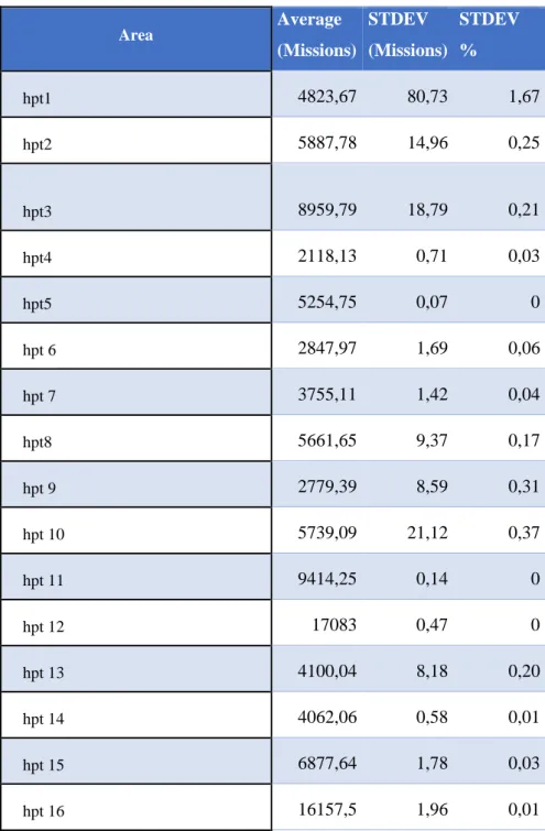
4.1.3 Model 4.10.157

The results from the model 4.10.157 had variations between ten equal runs, see table 2, 3 and 4.

Table 2. Average value and standard deviation for fatigue life. Model 4.10.157 for HPC.

Area Average (Missions) STDEV (Missions) STDEV (%) hpc1 7699,46 13,80 0,18 hpc2 7507,17 0,34 0,01 hpc3 9284,94 0,92 0,01 hpc4 13235 0 0 hpc5 13635 0 0 hpc6 4917,39 1,17 0,02 hpc7 4357,2 0,08 0 hpc8 20391,5 1,35 0,01 hpc9 13295 0 0 hpc10 8349,9 0 0

(22)

17

Table 3. Average value and standard deviation for fatigue life. Model 4.10.157 for HPT.

Area Average (Missions) STDEV (Missions) STDEV % hpt1 4823,67 80,73 1,67 hpt2 5887,78 14,96 0,25 hpt3 8959,79 18,79 0,21 hpt4 2118,13 0,71 0,03 hpt5 5254,75 0,07 0 hpt 6 2847,97 1,69 0,06 hpt 7 3755,11 1,42 0,04 hpt8 5661,65 9,37 0,17 hpt 9 2779,39 8,59 0,31 hpt 10 5739,09 21,12 0,37 hpt 11 9414,25 0,14 0 hpt 12 17083 0,47 0 hpt 13 4100,04 8,18 0,20 hpt 14 4062,06 0,58 0,01 hpt 15 6877,64 1,78 0,03 hpt 16 16157,5 1,96 0,01

(23)

18

Table 4. Average and standard deviation for fatigue life. Model 4.10.157 for LPT.

Area AVERAGE (Missions) STDEV (Missions) STDEV % lpt 1 14903,7 6,17 0,04 lpt 2 6279,41 80,57 1,28 lpt 3 9389,9 8,98 0,10 lpt 4 12551,4 8,28 0,07 lpt 5 15005,1 64,46 0,43 lpt 6 23494,7 20,57 0,09 lpt 7 7046,84 11,82 0,17 lpt 8 8502,02 34,80 0,41 lpt 9 8787,02 32,58 0,37

4.2 New models

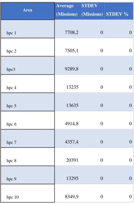
4.2.1 Model 4.10.124

The results from model 4.10.124 had small variations between the 10 runs. Look at table 5, 6 and 7.

(24)

19

Table 5. Average value and standard deviation for fatigue life. Model 4.10.124 for HPC.

Area Average (Missions) STDEV (Missions) STDEV % hpc 1 7708,2 0 0 hpc 2 7505,1 0 0 hpc3 9289,8 0 0 hpc 4 13235 0 0 hpc 5 13635 0 0 hpc 6 4914,8 0 0 hpc 7 4357,4 0 0 hpc 8 20391 0 0 hpc 9 13295 0 0 hpc 10 8349,9 0 0

(25)

20

Table 6. Average value and standard deviation for fatigue life. Model 4.10.124 for HPT

Area AVERAGE (Missions) STDEV (Missions) STDEV % hpt1 4863,06 0,07 0 hpt 2 6547,07 0,07 0 hpt 3 9623,54 0,13 0 hpt 4 2284,91 0,03 0 hpt 5 5258,1 0 0 hpt 6 3011,93 0,05 0 hpt 7 3760,31 0,09 0 hpt 8 6118,8 0 0 hpt 9 2705,42 0,06 0 hpt 10 6438,6 0 0 hpt 11 9420,9 0 0 hpt 12 17076 0 0 hpt 13 4093,75 0,09 0 hpt 14 4070,4 0 0 hpt 15 6888,1 0 0 hpt 16 16179 0 0

(26)

21

Table 7. Average value and standard deviation for fatigue life. Model 4.10.124 for LPT

Area AVERAGE (Missions) STDEV (Missions) STDEV % lpt 1 14899,6 0,70 0,01 lpt 2 5333,66 6,69 0,13 lpt 3 9343,95 0,05 0 lpt 4 12549,4 0,70 0 lpt 5 14693,8 0,79 0,01 lpt 6 23468 0 0 lpt 7 7008,98 0,06 0 lpt8 8483,17 0,11 0 lpt 9 8578,09 0,07 0

4.2.2 Model 4.10.160

The results from the run with model 4.10.160 had variations when the same mission was run in LAS ten times. By looking at area hpt10 there is a value who’s very big in comparison to other values from other models for this area and by looking closely at the results from all ten runs, see APPENDIX 4, a result for this area is marked as unreliable. If the standard deviation was calculated for area hpt10 but without this unreliable value it was equal to 56,33092 missions and the standard deviation in percent became 0,86%.

(27)

22

Table 8. Average value and standard deviation for fatigue life. Model 4.10.160 for HPT

Area Average (Missions) STDEV (Missions) STDEV % hpt1 3244,28 96,12 2,96 hpt 2 6519 34,03 0,52 hpt 3 10069,5 3,63 0,04 hpt 4 1939,52 0,56 0,03 hpt 5 6183,86 0,45 0,01 hpt 6 2983,93 1,41 0,05 hpt 7 3518,78 29,88 0,85 hpt 8 5710,61 34,69 0,61 hpt 9 2823,26 14,34 0,51 hpt 10 8,403E+26 2,66E+27 316,23 hpt 11 12050,2 2,62 0,02 hpt 12 18017 0 0 hpt 13 4061,38 27,36 0,67 hpt 14 3789,97 1,57 0,04 hpt15 7219,06 6,19 0,09 hpt 16 62088,5 74,61 0,12

The value from the test with model 4.10.160 that were marked unreliable were dramatically big and to see if this phenomenon occurs often the tests were made again several times. The same mission was run for a total of 50 times but this phenomenon only happened once.

(28)

23

4.2.2.1 Strain Analysis

A strain versus time diagram for area hpt10 was plotted for the run with an unreliable value (model 4.10.160). The results can be seen in figure 8. By looking at the y-axis there are negative values which means negative strain, that is a compressive force. At the time 1.4E03 seconds the negative strain is doing a jump from 3E-03 to about 7E-03 and is then decreasing until, again, a jump is seen from 6E-03 to about 2E-03. A new plot was made for this area but for another run with a reliable value for the fatigue life, see figure 9. In this plot there are positive strains that are increasing with time until it starts to approach the end then it’s decreasing. The phenomenon as occur in figure 8 only happened once out of 50 runs.

Figure 8. Run 8 for the area hpt10. The strain is doing a big jump in magnitude.

-8,00E-03 -7,00E-03 -6,00E-03 -5,00E-03 -4,00E-03 -3,00E-03 -2,00E-03 -1,00E-03 0,00E+00

0,00E+00 1,00E+03 2,00E+03 3,00E+03 4,00E+03 5,00E+03 6,00E+03

Str

ai

n

Time (Seconds)

(29)

24

Figure 9. Run 5 for area hpt10.

4.2.3 Model 4.10.173

For the tests with model 4.10.173 there were 3 runs that failed due to computer setup errors. The result is based on the seven runs that did succeed. The results contained variations between the equal runs.

0,00E+00 1,00E-03 2,00E-03 3,00E-03 4,00E-03 5,00E-03 6,00E-03 7,00E-03 8,00E-03 9,00E-03

0,00E+00 1,00E+03 2,00E+03 3,00E+03 4,00E+03 5,00E+03 6,00E+03

Str

ai

n

Time (Seconds)

(30)

25

Table 9. Average and standard deviation for fatigue life. Model 4.10.173 for HPT.

Area Average (Missions) STDEV (Missions) STDEV % hpt1 _2446,20 _20,73 _0,85 hpt2 3390,56 21,59 0,64 hpt3 _7658,30 _89,74 _1,17 hpt4 768,18 4,20 0,55 hpt5 6090,33 0,64 0,01 hpt6 3442,73 19,49 0,57 hpt7 _3908,84 _129,44 _3,31 hpt8 _4374,20 _17,64 _0,40 hpt9 4754,71 42,92 0,90 hpt10 9293,17 53,01 0,57 hpt11 _22766,14 _8,75 _0,04 hpt12 16424,29 6,73 0,04 hpt13 4298,66 14,43 0,34 hpt14 3887,13 2,52 0,06 hpt15 _7291,43 _6,23 _0,09 hpt16 40420,43 30,62 0,08

4.3 Time aspect

The time required for the calculations for the different components and models can be viewed in table 10,11 and 12. The time values in these tables are mean values from all runs.

Table 10. The time required for the calculations for HPC with different models.

Model Time (Mean value) 4.10.149 41h,11m,19s 4.10.167 65h,39m,9s 4.10.157 41h,15m,44s 4.10.124 41h,16m,14s

(31)

26

Table 11. The time required for the calculation for HPT with different models

Model Time (Mean

Value) 4.10.149 41h, 35m, 20s 4.10.157 25h, 13m, 26s 4.10.124 20h, 32m, 11s 4.10.160 16h, 9m, 26s 4.10.173 58h, 0m, 3s

Table 12. The time required for the calculation for LPT with different models

Model Time (Mean

Value) 4.10.149 6h, 33m, 32s

4.10.157 4h, 44m, 8s

(32)

27

5 Discussion

The goal is to have zero in standard deviation. It should not be variation in the result when same mission is run 10 times, that’s an uncertainty.

5.1 Old models

There was variations for the result for HPC with model 4.10.149, the results for tests with the same mission should preferably will be the same. There have been similar problems to update the models; the result has a variation that isn’t negligible. As can be seen for HPC with model 4.10.167 the results don’t change between different runs and the only thing that separates 4.10.149 and 4.10.167 is that 4.10.167 only runs with one core instead of two. The problem arises when two cores are used but in the best of worlds the model should use more cores because it shortens the calculation time. This can also be seen in the results. The model 4.10.149 doesn’t run with two cores for HPT and LPT and therefor the fatigue life results did not have any variations in the results between the equal runs.

For the model 4.10.157 there is variations in the results. The results from model 4.10.157 for HPC had less variation compared to HPT and LPT but the time for HPC did not change from model 4.10.149 either, this is because the model 4.10.149 is run with 2 cores for HPC so is 4.10.157.

5.2 New models

The results from the model 4.10.124 had less variations then 4.10.157 but there was still some small variation for the ten fatigue life.

Model 4.10.160 was made by an ANSYS expert. After runs with this model it can be seen that there were variations in the results when this model was used for the same mission several times. The results did still differ between the ten fatigue life values.

There was a value from the test with model 4.10.160 who were marked unreliable, by looking closely at the strain versus time diagram for this area it can be seen that the stress is negative, that is, a compressive force. This force did a jump in magnitude at the time 1,4E03. It’s a strange look for this type of diagram. There’s no explanation for why this happened but the inbuilt limits for reliable and unreliable results in LAS/LTS are important for LTS and its credibility. When a new strain versus time for the same area but in a different run was plotted with a reliable value the result is looking better. This is how this kind of diagram usually look like even though these diagrams always differ because they are based on real flight mission and every mission is different.

(33)

28

The model 4.10.173 that the ANSYS expert did also had variations that can not be neglected. Some of the runs with this model failed because the IT department has not managed to get the right set up of nodes yet for this ANSYS version. Because of that not all runs were succeeded the result files from LAS does not sum up. So to get the results from the seven runs that actually did succeed the files need to be manually treated. A MATLAB script for reading and match files to correct components were provided from the life management group at GKN. The reason why the result has variations can depend on several things and they are not all known. One problem is that the models converges to different solutions, this happens when the model uses more than one core. A theory is that something happens with the

communication when more than one core is used. It is a complex problem because the contact elements are non-linear. There are already converging requirements for the displacement globally but that does not seem to be enough. The problem seem to be on a local level. The problem with variations for the fatigue life between equal runs has been sent to ANSYS.

5.3 Time aspect

The time required for the calculations differed between the different models. For HPC the times are similar for all models except for the model 4.10.167. The model 4.10.167 is the same as 4.10.149 but it only runs with one core instead of two.

For LPT the time for the calculations were shortest for the model 4.10.157 and that’s because it’s run with two cores instead of one and the reason why model 4.10.124 takes as long as 4.10.149 is probably because new convergence requirements in this model.

For the component HPT the fastest model is 4.10.160, the slowest is with model 4.10.173. It can be seen that as more cores the models use the faster the calculations become but this conclusion does not fit with the results from model 4.10.173. Model 4.10.173 runs with four cores but has the longest duration. This is because the aim with the model 4.10.173 was to have a model without variation and because of that it has been built up with many

requirements so that the calculations converges to the right solution. Because of all these requirements, the model is heavier to run which leads to a longer duration for the calculations. The best would be to run with more cores but then the work with the models become harder because of the tendency to give variations in the results between runs for the same mission.

(34)

29

5.4 Method

Unfortunately, the set up and installation of the cluster got delayed and this project has a time limit so it has not been time for an investigation of the new cluster as was planned from the beginning. The expectation was also to find a good model for the latest version in ANSYS but it has been a struggle to come up with one. 4.10.173 is almost there but still a bit more way to go. Because of the struggle to find a good model, the delayed cluster and the problem with the results files for model 4.10.173 the work got a calm period in the middle of the project and more stressed at the end.

It has been hard to find references because of that LTS is a unique system to calculate life fatigue. GKN has five patent applications for LTS.

5.5 Future work

There is a need to continue with this work at GKN Aerospace so that they manage to come up with a model that works with the latest ANSYS version. It would be great if an ANSYS group tried to solve this together with the life management group at GKN.

The LTS-system is now only used for jet engines at GKN Aerospace but could be applied to other engines. In the future we may see LTS in the car industry or other industries. Or as Andersson, M writes in his public article “Life Tracking system (LTS) for RM12 [10]” in nuclear plants. LTS has several advantages as written below heading 2.3.2 Benefits with the Life Tracking System, LTS has a good sustainable impact. The users will be more aware of how the usage of the, in this case, jet engine will affect the life consumptions and of course they want to replace their components as rarely that’s possible because of economic aspects and this is also good in a sustainable aspect. A more kinder way to use the engine, or a cheaper way seen from life consumption aspect is often also better for the environment because of reduced emissions.

The work with a new model has been moving forward for HPT and there is a need to do the same with both HPC and LPT. Then a validation needs to be done for these components too. As mentioned before, the system LTS could be applied to other industries and it would be interesting to do a project about LTS future applications.

(35)

30

6 Conclusions

• The model 4.10.149 has variations when the same mission was run ten times for the component HPC.

• Both the model 4.10.160 and 4.10.173 had variation in the results when the same mission was run for ten times.

• When the tests are run with two or more cores the problem with a variation in the results occurs.

• The time required for the calculations was shorter when the test was made with a model that runs with more cores except for the model 4.10.173 that has many requirements in the calculation model.

(36)

31

7 Acknowledgements

I want to thank Christian Lundh, manager at the life management department at GKN Aerospace who gave me this opportunity to do my bachelor thesis with them. I also want to thank my supervisor at GKN, Magnus Andersson, for all the help he gave me within this project. This help meant a lot to me to finish this thesis, he helped me with the program LAS and provided me with good references to write my report.

I also want to thank the life management group at GKN aerospace for the kind treatment. I also want to thank my supervisor, Henrik Jackman, at Karlstad University for the guidance during this project.

(37)

32

8 References

[1] GKN Aerospace AB. About GKN [Internet]. Redditch:GKN plc;[Date unknown]. Available from: https://www.gkn.com/en/about-gkn/, 2018-04-26.

http://www.gkngroup.com/GKNSweden/aerospace/Pages/default.aspx, 2018-04-25.

http://www.gkngroup.com/GKNSweden/aerospace/produkter/Pages/default.aspx, 2018-04-25.

[4] Alsen G. Gripen [Picture]. Trollhättan. Alsen Geryll; 2018-05-16.

[5] GKN Aerospace AB. GKN Engines [Internet]. Redditch: GKN plc; [Date Unknown] Available from: https://www.gkn.com/en/our-divisions/gkn-aerospace/our-solutions/engines/, 2018-01-18

http://www.gkngroup.com/GKNSweden/aerospace/produkter/Pages/flygmotorer.aspx,

2018-04-25.

(38)

33

[8] Sundström B. Handbok och formelsamling i hållfasthetslära. Ed eight. Stockholm: Instant Book AB;2013

[9] Andersson M, Svensson P, Wänman F. Determining life consumption of a mechanical part. Trollhattan; US 2015/0234951 A1, 2015-08-20.

[10] Andersson M. Life Tracking System (LTS) for RM12[Internet]. Trollhattan: Volvo Aero Corporation;2011.1803

[11] Wänman F. Life Tracking System [Intern material]. Trollhattan: GKN Aerospace Sweden AB; 20160407.

[12] Femto Engineering. In FEA, what is linear and nonlinear analysis? [Internet]. Oude delf: Femto Engineering; [Date unknown]. Available from: https://www.femto.eu/stories/linear-non-linear-analysis-explained/, 2018-05-20.

[13] Metrisin J. Guidelines for obtaining contact convergence [Powerpoint presentation on the Internet]. Pennsylvania; ANSYS, Inc; ©2008 . Avaiable from: https://www.ansys.com/- /media/ansys/corporate/resourcelibrary/conference-paper/2008-int-ansys-conf-guidelines-contact-convergence.pdf, 2018-05-20.

(39)

34

(40)

35

(41)

36

(42)

37

(43)

38

(44)

39

(45)

40

A study of calculation models for fatigue life prediction