Explaining rifle shooting factors through multi-sensor body tracking : Using transformers and attention to mine actionable patterns from skeleton graphs

Explaining rifle shooting

factors through multi-sensor

body tracking

Using transformers and attention

to mine actionable patterns from

skeleton graphs

PAPER WITHIN Product Development AUTHORS: Filip Andersson, Jonatan Flyckt TUTOR: Niklas Lavesson

Examiner: Vladimir Tarasov Supervisor: Niklas Lavesson

Scope: 30 credits

Date: 2021-06-17

Mailing address: Visiting address: Phone:

Box 1026 Gjuterigatan 5 036-10 10 00

Abstract

There is a lack of data-driven training instructions for sports shooters, as instruction has commonly been based on subjective assessments. Many studies have correlated body posture and balance to shooting performance in rifle shooting tasks, but most of them have focused on single aspects of postural control. This thesis has focused on finding relevant rifle shooting factors by examining the entire body over sequences of time. We performed a data collection with 13 human participants who carried out live rifle shooting scenarios while being recorded with multiple biometric sensors, including several body trackers. An experiment was conducted to identify what aspects of rifle shooting could be predicted and explained using these data. We employed a pre-processing pipeline to produce a novel skeleton sequence representation, and used it to train a transformer model. The predictions from this model could be explained on a per sample basis using the attention mechanism, and visualised in an interactive format for humans to interpret. It was possible to separate the different phases of a shooting scenario from body posture with a high classification accuracy (81%). However, no correlation could be shown between shooting performance and body posture from our data. Future work could focus on novel feature engineering, and on examining alternative machine learning approaches. The dataset and pre-processing pipeline, as well as the techniques for generating explainable predictions presented in this thesis has laid the groundwork for future research in the sports shooting domain.

Keywords

Acknowledgements

We wish to thank Professor Niklas Lavesson for guidance and supervision that helped us shape this thesis project from beginning to end. We also wish to thank Andreas M˚ansson at Saab AB, Training and Simulation for his enthusiasm and support, without which this project would not have been possible. Thank you to our co-students Max Pettersson and Saga Bergdahl, whose collaboration in both ideas and the execution of this thesis was valuable and rewarding. A big thank you to Anders Johanson, Per Lexander, Olof Bengtsson, Robert Andr´en, and everyone else at Saab AB, Training and Simulation who have assisted in the data collection and idea stages of this thesis project. We also wish to express our gratitude to the 13 anonymous participants who took part in our data collection. Thank you also to Dr. Florian Westphal for technical feedback helping our approach in the right direction. This work has been performed within the Mining Actionable Patterns from complex Physical Environments (MAPPE) research project in collaboration with J¨onk¨oping Univeristy and Saab AB, Training and Simulation, and was funded by the Knowledge Foundation.

Contents

1 Introduction 1

1.1 Aim and scope . . . 1

2 Background 3 2.1 Shooting . . . 3

2.2 Transfer learning . . . 3

2.3 Classical machine learning techniques for sequential data . . . 3

2.4 Transformers . . . 4

3 Related work 5 3.1 Postural stability and shooting performance . . . 5

3.2 Kinect and body tracking in scientific research . . . 5

3.3 Action classification . . . 5

4 Scientific Method 7 4.1 Experiment . . . 7

4.2 Validity threats and confounding factors . . . 7

5 Data collection 8 6 Technical approach 12 6.1 Data pre-processing . . . 12

6.2 Feature embedding and ViT adaptation . . . 15

6.3 Shooting pose estimation . . . 15

6.4 Shooting performance estimation . . . 16

7 Results and analysis 18 7.1 Pose estimation . . . 18

7.2 Shooting performance estimation . . . 20

8 Discussion 21 8.1 Future work . . . 22

9 Conclusions 24

References 25

1

Introduction

There are many factors affecting a shooter’s performance in rifle shooting. Important factors are time spent in the aiming process, weapon movement before triggering, and body postural sway as a result of poor balance (Mason, Cowan, & Gonczol, 1990). Because the eyes are focused on the target at the moment of shooting, they can not be used to control postural stability (Aalto, Pyykk¨o, Ilmarinen, K¨ahk¨onen, & Starck, 1990). Several studies correlate poor posture control with poor shooting results for rifle shooting (Ball, Best, & Wrigley, 2003; Era, Konttinen, Mehto, Saarela, & Lyytinen, 1996; Mononen, Konttinen, Viitasalo, & Era, 2007; Sattlecker, Buchecker, M¨uller, & Lindinger, 2014). These studies mainly define posture control as body sway calculated from the force exerted by each foot on the ground measured with force plates. Because only balance in the legs are measured, these force plate sensors may not produce the full picture for the entire body’s postural control. The force plates also restrict the subject to a stationary position. Therefore, it is interesting to examine other approaches that could be taken to gain a more comprehensive understanding of how postural stability affects shooting performance. Bio-mechanic pose estimation has been researched for almost half a century, often by using physical markers placed on human participants to build 3D body representations from visual sensors (Johansson, 1973). New techniques developed during the the last decade allow for the tracking of joints by using image processing and machine learning. These technologies can build accurate 3D depth maps, producing so called skeletons of interconnected body joints. A relatively low-cost commercial sensor in this area is the Kinect body tracking sensor (Shotton et al., 2013), which uses image and depth data with machine learning to build robust, view invariant skeleton models that measure 3D trajectories of human skeleton joints over time (Shotton et al., 2013). The latest version: Azure Kinect, is available since 2019.

As a result of these accurate low-cost technologies, the use of skeleton data together with machine learning is studied more actively, especially in the area of action recognition (Du, Wang, & Wang, 2015; Ke, Bennamoun, An, Sohel, & Boussaid, 2017; Tang, Tian, Lu, Li, & Zhou, 2018; Xia, Chen, & Aggarwal, 2012; Yan, Xiong, & Lin, 2018). Skeleton data can also successfully measure motor functions (Otte et al., 2016), postural stability (Clark et al., 2015; Dehbandi et al., 2017; Leightley et al., 2016), as well as to some extent assess skill level in sports, e.g. handball (Elaoud, Barhoumi, Zagrouba, & Agrebi, 2020). There is a scientific consensus that postural balance is an important factor for rifle shooting performance (Aalto et al., 1990; Ball et al., 2003; Era et al., 1996; Ko, Han, & Newell, 2018; Mononen et al., 2007). Therefore, it is interesting to examine whether there are other postural factors besides postural sway that affect shooting performance, as such knowledge could be of assistance during the training of novice shooters.

1.1

Aim and scope

There is a research gap in machine learning approaches for skeleton data that explain their reasoning, as well as in using machine learning for decision support within the sports shooting domain. We design a fully encompassing workflow ranging from data collection in live shooting tasks, to sensor merging, data processing, and the construction of explainable machine learning models. The attention mechanism in the deep learning transformer architecture is used to gain insights into what the model focuses on when it makes certain predictions (Vaswani et al., 2017). This thesis will attempt to answer the research question:

Can relevant factors for rifle shooting tasks be determined through posture and body movements? It is expected that, as a result of the proposed work, an increased understanding is gained of how to model experiments for shooting scenarios that use multiple biometric sensors. The thesis will identify the possibilities and limitations with the gathered skeleton data, as well as give an initial insight into how skeleton data from live shooting scenarios can be modelled to generate explainable and relevant factors.

This thesis is performed in collaboration with Saab AB, Training and Simulation, who is an industry partner in the MAPPE research project conducted by J¨onk¨oping University. In this project, Saab is interested in exploring the potential of novel sensor technologies for providing complementary information

about the conditions of live fire exercises and performance of shooters. Saab is also interested in investigating the possible use of intelligent methods and tools (artificial intelligence, machine learning, and data mining) to support analysis of data gathered during exercises to provide decision support and feedback to shooters and instructors.

2

Background

This section will cover the background for the sports shooting domain, as well as the machine learning techniques that are used throughout this thesis. To provide motivation for some of our design choices, we will also discuss some of the relevant machine learning techniques that have led up to the current state-of-the-art.

2.1

Shooting

Sports shooting can be broadly divided into two domains: static shooting and dynamic shooting. This thesis focuses on dynamic shooting, which has a higher level of complexity with movements of both the shooter and targets. Both static and dynamic rifle shooting training is commonly conducted with one or multiple practitioners being instructed by a supervisor. For novices, training is mostly focused on striking static targets at fixed distances, where a supervisor focuses on factors such as stability, aiming, control, and movement (Goldberg, Amburn, Ragusa, & Chen, 2017). Different shooting instructors can be inconsistent in their feedback due to personal biases in the interpretation of data (James & Dyer, 2011). Consequently, there is a need for an objective and consistent data-driven feedback based on statistical analysis of data from real shooting scenarios.

2.2

Transfer learning

Many deep learning tasks suffer from a lack of sufficient training data, often resulting in poor performance and overfitting. To combat this, knowledge can be transferred to the desired domain from pre-trained models from similar domains by using transfer learning. The limited data from the narrow domain is then used to help the model specialise and fine-tune its parameters. There are many different transfer learning approaches, some of the more common ones focus on transferring feature representations or parameters. When transferring parameter weights, the training process that uses the specialised data is given a head start. Because the general knowledge is already represented in the model weights, the training can focus on learning the finer details. (Pan & Yang, 2010)

2.3

Classical machine learning techniques for sequential data

Sequential data in machine learning tasks require either heavy temporal related feature engineering, or the use of techniques capable of dealing with sequences by other means than fixed-length vector representations. A Recurrent Neural Network (RNN) is a deep learning model relying on hidden unit patterns feeding back into themselves through recurrent links, allowing the network to remember previous iterations and to map long temporal relationships (Elman, 1990). Despite their ability to represent temporal contexts, RNNs are limited in their training capabilities, as long-term relations can sometimes cause very large gradient values, resulting in unstable models (Bengio, Frasconi, & Simard, 1993). Long Short-Term Memory(LSTM) networks attempt to overcome these issues by introducing a new type of memory cell called the forget gate, capable of remembering long-term dependencies for as long as is needed (Hochreiter & Schmidhuber, 1997). However, as more parameters are introduced, LSTMs become more prone to overfitting than classical RNNs (Du et al., 2015).

Sequential data that are represented as graphs (e.g. body tracking skeletons) can use Graph Convolutional Networks (GCNs) and connect nodes through both the spatial and temporal domains. GCNs extract relevant information from the graph as a whole by smoothing out connected nodes, and propagating their values throughout the graph either in a directed or an undirected fashion (Wu et al., 2021). This smoothing reduces local noise, but may also remove relevant small-scale features if too many layers are used (Chen et al., 2020).

2.4

Transformers

A Transformer is a non-RNN model for sequential data, which can often remember early information in long sequences of data better than LSTMs (Vaswani et al., 2017). Transformers do not have an internal state, making them easily parallelisable during training. Instead, they rely solely on an attention mechanism which computes the correlation of the input to a desired output. This is accomplished by computing the similarity of a set of query and key vectors using their dot products, producing a set of value vectors. From these value vectors, attention matrices are calculated which map the strength of connection between input feature embeddings throughout the network layers. These attention matrices have the added benefit of being able to explain some of the model’s reasoning. Standard transformers use an encoder-decoder architecture, and are composed of several stacked self-attention layers. During training, the encoder receives an input vector including positional tokens representing each embedding’s position in the sequence, and the decoder receives a target output embedding. This architecture is used for general natural language processing (NLP), e.g. in translation, summarisation, and sentiment analysis tasks. A trained NLP encoder can therefore be seen as a general representation of the natural language, characterising relevant features from sequences of words.

Transformers are not limited to natural language; Vision Transformers (ViTs) are a novel technique specifically designed to handle images (Dosovitskiy et al., 2021). ViTs divide images into equally sized rectangular patches, and embed them into projected one-dimensional vector representations by feeding them through trainable embedding layers. These embeddings are then treated in the same way as positional tokens in a standard transformer. Compared to other state-of-the-art computer vision algorithms such as convolutional neural networks (CNNs), ViTs can focus more on the global aspects of an image, whereas CNNs are restricted, and thus more biased to local neighbourhoods. Similarly to standard transformers, ViTs can explain their predictions by using the attention produced from patch embeddings. ViTs do not use a decoder, and instead opt for using a simple multi-layer perceptron (MLP) tailored for the specific learning task after the encoder layers. Because ViTs need to learn local relations from a global perspective, they often require large amounts of training data compared to CNNs. ViTs also require more computational resources during training and inference. However, this requirement can be reduced by increasing the size of the patches, as the model increases in size quadratically from the number of feature embeddings. We use Vision Transformers in this thesis due to their ability to map long term sequences of data, as well as our goal of explaining what factors affect shooting performance.

3

Related work

3.1

Postural stability and shooting performance

Several studies have used force plate sensors to measure posture control in shooting tasks. However, these force plates are prohibitively expensive and can be impractical in situations outside controlled research studies and clinical environments (Yeung, Cheng, Fong, Lee, & Tong, 2014). The studies that have examined body tracking in shooting tasks have had a delimited approach, mainly focusing on correlating shooting performance to mean sway velocity calculated from joint angles (Sattlecker et al., 2014). Skilled and experienced shooters have generally shown a better postural stability than novices (Aalto et al., 1990; Era et al., 1996; Mononen et al., 2007). Gun barrel stability has also been correlated to postural stability by several studies (Era et al., 1996; Mononen et al., 2007; Sattlecker et al., 2014). Although some studies have correlated posture to shooting performance between individuals (Era et al., 1996), other studies have only shown intra-individual correlations (Ball et al., 2003). These conflicting results, as well as a general lack of studies examining the effects of the posture and movements of the entire body on shooting performance, motivate further study.

3.2

Kinect and body tracking in scientific research

The Azure Kinect sensor (Shotton et al., 2013) is a viable low-cost alternative to classical marker-based motion capture systems (Clark et al., 2015) as well as force plates (Dehbandi et al., 2017) for measuring balance. Compared to motion capture suits, the Kinect has performed moderately to excellently depending on the tasks. The upside is that the participants are not restricted by wearing a motion capture suit. However, poorer tracking of the feet and ankles has been observed (Clark et al., 2015; Otte et al., 2016). The Kinect sensor holds up well as a balance measurement when compared to force plate sensors (Clark et al., 2015; Dehbandi et al., 2017), sometimes even outperforming them, with the upside of not limiting subjects to a stationary position. Downsides are limitations in accurately representing anterior-posterior swaying movements, overestimating large swaying movements, and having a framerate that is limiting for certain tasks (Sgr`o, Nicolosi, Schembri, Pavone, & Lipoma, 2015).

We found very few studies using skeleton data to assess skill levels in humans, despite an exhaustive literature search. Most such studies have focused on isolated aspects of the body, such as angles between key joints in handball throws (Elaoud et al., 2020), or the take-off velocity of jumping motions (Sgr`o et al., 2015).

Because of occluded joints forcing the Kinect sensor to estimate positions, Gao, Yu, Zhou, and Du (2015) found that using two Kinect sensors placed in front of the target at an angle led to higher body tracking accuracy. N´u˜nez, Cabido, Pantrigo, Montemayor, and V´elez (2018) proposed data augmentations on the skeleton data by shifting the graph slightly, because limited amounts of data would cause generalisability issues for machine learning models. Vemulapalli, Arrate, and Chellappa (2014) suggested that model performance could be improved by making the skeletons invariant to the absolute locations of subjects. They did this by transforming the coordinates to a body-centric view with the hip center as the origin, and the x-axis running parallel to the hip.

3.3

Action classification

Action classification tasks use time-series skeleton data, often with deep learning techniques, to classify human actions such as jumping, running, throwing etc. This section provides a brief chronological survey of the area.

Du et al. (2015) used a hierarchically bi-directional RNN approach, and found that it was beneficial to divide the skeleton into five body parts (arms, legs, torso) before fusing them iteratively into one feature representation. Liu, Shahroudy, Xu, and Wang (2016) achieved good results with LSTMs and hierarchical tree traversal techniques, in large part due to the LSTM’s inherent strengths in discarding irrelevant information such as weak sensor data. Adding the attention mechanism to this approach improved the LSTMs global context memory and increased predictive performance (Liu, Wang, Hu,

Duan, & Kot, 2017). Attention has also been able to locate the most discriminative time frames across longer sequences of skeletons, e.g. being able to identify the point at which the arm begins to stretch in a punching motion (Song, Lan, Xing, Zeng, & Liu, 2017).

Ke et al. (2017) used convolutional neural networks (CNNs) to classify actions with skeleton data, arguing that they could remember long time sequences better than LSTMs. They restructured skeleton sequences into three cylindrical coordinate channels, each composed of four frames. Convolutions on graphs have also been used to automatically extract feature maps from joints connected spatially between each other, as well as temporally through time (Yan et al., 2018). Plizzari, Cannici, and Matteucci (2020) combined a high level local feature extracting GCN with transformers and self-attention, allowing for explanations of what features were mutually important for predictions, as well as alleviating the long temporal relation issues of LSTMs (Vaswani et al., 2017). They separated the temporal and spatial skeleton graphs into separate streams, similarly to Song et al. (2017), which allowed the model to attend both to the important time frames and the joints with the most discriminative power.

4

Scientific Method

4.1

Experiment

The research question will be answered with the help of an experiment. The hypotheses for the experiment are:

1. It is possible to separate the different phases of a rifle shooting scenario with body tracking data. 2. There is a correlation between body postures as measured by body tracking sensors, and rifle

shooting performance.

This experiment will rely on data gathered from several human participants. The participants will perform a rifle shooting task, as described in the Data collection section. The experiment is a quasi-experiment, meaning that there will be no random assignment, and that the potentially discovered relations in the data may not be true cause and effect relations (Shadish, Cook, & Campbell, 2002). The experiment will be controlled in the sense that we will have full control over the manipulation of the data, and can perform as many iterations as needed. The dependent variables for the experiment will be the shooting performance of the test participant, expressed as a continuous score variable ranging between zero and one, as well as different identified shooting poses. The score variable will be a combination of shooting accuracy and time taken. The independent variables will be the sequential body tracking data produced by the Azure Kinect sensors.

4.2

Validity threats and confounding factors

The data collection and experiment have several possible confounding factors that may affect the results: External validity threats: Because we will have relatively few participants in the shooting scenario, the data may be skewed to one type of behaviour, and the results may therefore not be statistically relevant. Most of the participants will be males in the 40-55 year age range with a military training background. This means that it may be difficult to generalise the results from outside of these groups.

Internal validity threats: The wearable sensors equipped on the participants and weapon may produce an artificial situation, which can affect the participants’ movement and shooting behaviour.

Statistical validity threats: Our confidence intervals will be based on the computed metrics for each separate cross validation fold (one fold per participant). This means that there may be a bias in the interval, as some participants will have more skeleton sequence samples than others due to taking a longer time to complete the scenario.

Construct validity threats: Poor sensor readings are a potential confounding factor, which is one of the reasons that we will use three Kinect sensors as described in the Data collection section. Our automatic labelling of poses by using shot times is also a validity threat, as some classes will inevitably be incorrectly labelled for training and testing. Our regression target variable will not be an absolutely accurate measure of skill, but rather an estimation based on the available shooting performance data.

5

Data collection

The data collection for this thesis relied on one well-defined scenario, with a focus on identifying the postural effects on shooting performance with a semi-automatic rifle. We performed the data collection together with another thesis, which focused on the effects of eye movements and weapon handling in shooting tasks. The data collection was performed in an indoor shooting range to limit the effects of weather and wind on our participants and sensors. To fulfil the goals of both theses, we designed a scenario that could measure both reaction time and shooting performance when switching between different shooting targets and body postures (Figure 1).

Scenario description:

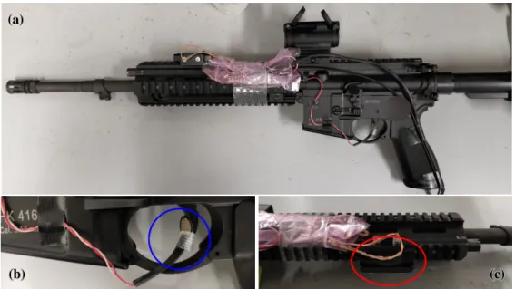
1. The participant is equipped with a semi-automatic rifle (HK416 with a 5.56 mm x 45 calibre) (Figure 2a).

2. Two pop-up targets are placed 20 metres away from the shooter, with roughly 1.5 metres between each other (Figure 3a).

3. The participant starts in a standing, shooting ready position.

4. The left target pops up, the participant aims at the target and fires a set of three shots. 5. The participants switches back to a shooting ready position.

6. 15 seconds after the left target popped up, the right target pops up. The participant switches targets and fires a set of three shots at the right target.

7. The participant switches to a kneeling position.

8. The participant fires another set of three shots at the right target.

9. The participant switches targets and fires a final set of three shots at the left target. 10. The participant secures and unloads the weapon.

1

2

4

5

6

3

Figure 1. Scenario illustration. Sequential illustration of the shooting scenario for the data collection. Source: Pettersson (2021).

Figure 3b shows the shooting target that was used in the data collection scenario. The participants were instructed to hit as close to the centre as possible while still maintaining a high speed of execution. The zone scores communicated to the shooters were: five points for hitting the inner zone, three points for the middle zone, one point for the outer zone, and -10 points for missing the target. It was also communicated that this score would be divided by time of completion in seconds.

(a) (a) (a) (a) (a) (a) (a) (a) (a) (a) (a) (a) (a) (a) (a) (a) (a) (a) (a) (a) (a) (a) (a)(a)(a)(a)(a)(a)(a)(a)(a)(a)(a)(a)(a)(a)(a)(a)(a)(a)(a)(a)(a)(a)(a)(a)(a)(a)(a)(a)(a)(a)(a)(a)(a)(a)(a)(a)(a)(a)(a)(a)(a)(a)(a)(a)(a)(a)(a)(a)(a)(a)(a)(a)(a)(a)(a)(a)(a)(a)(a)(a)(a)(a)(a)(a)(a)(a)(a)(a)(a)(a)(a)(a)(a)(a)(a)(a)(a)(a)(a)(a)(a)(a)(a)(a) (a) (a) (a) (a) (a) (a) (a) (a) (a) (a) (a) (a) (a) (a) (a) (a) (a) (a) (a) (a) (a) (a) (a) (a) (a) (a) (a) (a) (a) (a) (a) (a) (a) (a) (a) (a) (a) (a) (a) (a) (a) (a) (a) (a) (a) (a) (a) (a) (a) (a) (a) (a) (a) (a) (a) (a) (a) (a) (a) (a) (a) (a) (a) (a) (a) (a) (a) (a) (a) (a) (a) (a) (a) (a) (a) (a) (a) (a) (a) (a) (a) (a) (a) (a) (a) (a) (a) (a) (a) (a) (a) (a) (a) (a) (a) (a) (a) (a) (a) (a) (a) (a) (a) (a) (a) (a) (a) (a) (a) (a) (a) (a) (a) (a) (a) (a) (a) (a) (a) (a) (a) (a) (a) (a) (a) (a) (a) (a) (a) (a) (a) (a) (a) (a) (a) (a) (a) (a) (a) (a) (a) (a) (a) (a) (a) (a) (a) (a) (a) (a) (a) (b) (b) (b) (b) (b) (b) (b) (b) (b) (b) (b) (b) (b) (b) (b) (b) (b) (b) (b) (b) (b) (b) (b) (b) (b) (b) (b) (b) (b) (b)(b)(b)(b)(b)(b)(b)(b)(b)(b)(b)(b)(b)(b)(b)(b)(b)(b)(b)(b)(b)(b)(b)(b)(b)(b)(b)(b)(b)(b)(b)(b)(b)(b)(b)(b)(b)(b)(b)(b)(b)(b)(b)(b)(b)(b)(b)(b)(b)(b)(b)(b)(b)(b)(b)(b)(b)(b)(b)(b)(b)(b)(b)(b)(b)(b)(b)(b)(b)(b) (b) (b) (b) (b) (b) (b) (b) (b) (b) (b) (b) (b) (b) (b) (b) (b) (b) (b) (b) (b) (b) (b) (b) (b) (b) (b) (b) (b) (b) (b) (b) (b) (b) (b) (b) (b) (b) (b) (b) (b) (b) (b) (b) (b) (b) (b) (b) (b) (b) (b) (b) (b) (b) (b) (b) (b) (b) (b) (b) (b) (b) (b) (b) (b) (b) (b) (b) (b) (b) (b) (b) (b) (b) (b) (b) (b) (b) (b) (b) (b) (b) (b) (b) (b) (b) (b) (b) (b) (b) (b) (b) (b) (b) (b) (b) (b) (b) (b) (b) (b) (b) (b) (b) (b) (b) (b) (b) (b) (b) (b) (b) (b) (b) (b) (b) (b) (b) (b) (b) (b) (b) (b) (b) (b) (b) (b) (b) (b) (b) (b) (b) (b) (b) (b) (b) (b) (b) (b) (b) (b) (b) (b) (b) (b) (b) (b) (b) (b) (b) (b) (b) (b) (b) (b) (b) (b) (b) (b) (c)(c)(c)(c)(c)(c)(c)(c)(c)(c)(c)(c)(c)(c)(c)(c)(c)(c)(c)(c)(c)(c)(c)(c)(c)(c)(c)(c)(c)(c)(c)(c)(c)(c)(c)(c)(c)(c)(c)(c)(c)(c)(c)(c)(c)(c)(c)(c)(c)(c)(c)(c)(c)(c)(c)(c)(c)(c)(c)(c)(c)(c)(c)(c)(c)(c)(c)(c)(c)(c)(c)(c)(c)(c)(c)(c)(c)(c)(c)(c)(c)(c)(c)(c)(c)(c)(c)(c)(c)(c)(c)(c)(c)(c)(c)(c)(c)(c)(c)(c)(c)(c)(c)(c)(c)(c)(c)(c)(c)(c)(c)(c)(c)(c)(c)(c)(c)(c)(c)(c)(c)(c)(c)(c)(c)(c)(c)(c)(c)(c)(c)(c)(c)(c)(c)(c)(c)(c)(c)(c)(c)(c)(c)(c)(c)(c)(c)(c)(c)(c)(c)(c)(c)(c)(c)(c)(c)(c)(c)(c)(c)(c)(c)(c)(c)(c)(c)(c)(c)(c)(c)(c)(c)(c)(c)(c)(c)(c)(c)(c)(c)(c)(c)(c)(c)(c)(c)(c)(c)(c)(c)(c)(c)(c)(c)(c)(c)(c)(c)(c)(c)(c)(c)(c)(c)(c)(c)(c)(c)(c)(c)(c)(c)(c)(c)(c)(c)(c)(c)(c)(c)(c)(c)(c)(c)(c)(c)(c)(c)(c)(c)(c)(c)(c)(c)(c)(c)(c)(c)(c)(c)(c)(c)(c)(c)(c)(c)(c)(c)(c)(c)(c)(c)(c)(c)(c)(c) Figure 2. HK416.

(a): The HK416 semi-automatic rifle (5.56 mm x 45 calibre) used in the data collection scenario. (b): Trigger pull force sensor placement.

(c): Weapon accelerometer placement.

(a) (a) (a) (a) (a) (a) (a) (a) (a) (a) (a)(a)(a)(a)(a)(a)(a)(a)(a)(a)(a)(a)(a)(a)(a)(a)(a)(a)(a)(a)(a)(a)(a)(a)(a)(a)(a)(a)(a)(a)(a)(a)(a)(a)(a)(a)(a)(a)(a)(a)(a)(a)(a)(a)(a)(a)(a)(a)(a)(a)(a)(a)(a)(a)(a)(a)(a)(a)(a)(a)(a)(a)(a)(a)(a)(a)(a)(a)(a)(a)(a)(a)(a)(a)(a)(a)(a)(a)(a)(a)(a)(a)(a)(a)(a)(a)(a)(a)(a)(a)(a)(a)(a)(a)(a)(a)(a)(a)(a)(a)(a)(a)(a)(a)(a)(a)(a)(a) (a) (a) (a) (a) (a) (a) (a) (a) (a) (a) (a) (a) (a) (a) (a) (a) (a) (a) (a) (a) (a) (a) (a) (a) (a) (a) (a) (a) (a) (a) (a) (a) (a) (a) (a) (a) (a) (a) (a) (a) (a) (a) (a) (a) (a) (a) (a) (a) (a) (a) (a) (a) (a) (a) (a) (a) (a) (a) (a) (a) (a) (a) (a) (a) (a) (a) (a) (a) (a) (a) (a) (a) (a) (a) (a) (a) (a) (a) (a) (a) (a) (a) (a) (a) (a) (a) (a) (a) (a) (a) (a) (a) (a) (a) (a) (a) (a) (a) (a) (a) (a) (a) (a) (a) (a) (a) (a) (a) (a) (a) (a) (a) (a) (a) (a) (a) (a) (a) (a) (a) (a) (a) (a) (a) (a) (a) (a) (a) (a) (a) (a) (a) (a) (a) (a) (a) (a) (a) (a) (b)(b)(b)(b)(b)(b)(b)(b)(b)(b)(b)(b)(b)(b)(b)(b)(b)(b)(b)(b)(b)(b)(b)(b)(b)(b)(b)(b)(b)(b)(b)(b)(b)(b)(b)(b)(b)(b)(b)(b)(b)(b)(b)(b)(b)(b)(b)(b)(b)(b)(b)(b)(b)(b)(b)(b)(b)(b)(b)(b)(b)(b)(b)(b)(b)(b)(b)(b)(b)(b)(b)(b)(b)(b)(b)(b)(b)(b)(b)(b)(b)(b)(b)(b)(b)(b)(b)(b)(b)(b)(b)(b)(b)(b)(b)(b)(b)(b)(b)(b)(b)(b)(b)(b)(b)(b)(b)(b)(b)(b)(b)(b)(b)(b)(b)(b)(b)(b)(b)(b)(b)(b)(b)(b)(b)(b)(b)(b)(b)(b)(b)(b)(b)(b)(b)(b)(b)(b)(b)(b)(b)(b)(b)(b)(b)(b)(b)(b)(b)(b)(b)(b)(b)(b)(b)(b)(b)(b)(b)(b)(b)(b)(b)(b)(b)(b)(b)(b)(b)(b)(b)(b)(b)(b)(b)(b)(b)(b)(b)(b)(b)(b)(b)(b)(b)(b)(b)(b)(b)(b)(b)(b)(b)(b)(b)(b)(b)(b)(b)(b)(b)(b)(b)(b)(b)(b)(b)(b)(b)(b)(b)(b)(b)(b)(b)(b)(b)(b)(b)(b)(b)(b)(b)(b)(b)(b)(b)(b)(b)(b)(b)(b)(b)(b)(b)(b)(b)(b)(b)(b)(b)(b)(b)(b)(b)(b)(b)(b)(b)(b)(b)(b)(b)(b)(b)(b)(b)

Figure 3. Targets and shot detection system.

(a): The yellow and red squares show the left and right pop-up targets used in the data collection. The blue square shows the LOMAH system (“Saab AB, Training and Simulation”, 2019), responsible for detecting shot positions. (b): The International Practical Shooting Confederation (IPSC) target plate with scoring zones that was used in the data collection, the size of an A4 paper sheet.

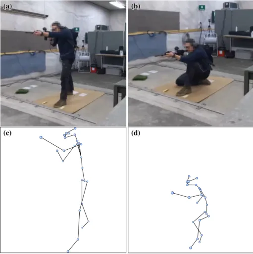
For a robust and diverse dataset, it would have been ideal to have shooting participants of different experience levels. However, due to safety constraints, only experienced shooters with official weapons training could participate. We used 13 shooters in the data collection, 12 of whom had a military background, three of whom had a sports shooting background, and three of whom had a background in hunting. All participants were male, and ranged from the age of 31 to 62, with an average age of 48. To preserve anonymity, each shooter was assigned a random identification letter (A-M). Due to the importance of a diverse dataset when training machine learning models, we attempted to simulate poor posture by having the participants perform half of the scenarios with their non-dominant hand. Each participant performed the scenario six times, resulting in a total number of 78 recorded shooting scenarios. Figure 4(a,b) shows a participant performing the scenario.

The Azure Kinect body tracking sensor (Shotton et al., 2013) was used to capture the body movements of the participants during the scenario. The accuracy of the Kinect sensor can be affected by several factors such as occlusion of body parts, e.g. a hand behind the body from the view of the camera. Other factors include poor lighting conditions, or disruption of the sensors’ infrared signals from e.g. sunlight or

infrared heaters. To mitigate the effects of poor sensor readings, we used three Kinect sensors: one behind the participant, and two to the front on either side of the participant at roughly a 45◦angle, as suggested by Gao et al. (2015). The sensor behind the participant was placed slightly to the right, because when placed straight behind the participant, the sensor would have difficulties with determining in which direction the participant was facing. To ensure a consistent and coordinated trigger timing of 30 frames per second on all three devices, the Kinect sensors were connected together with a synchronisation wire signalling when to capture new frames.

(a) (a) (a) (a) (a) (a) (a) (a) (a) (a) (a) (a) (a) (a) (a) (a) (a) (a) (a) (a) (a) (a) (a) (a) (a) (a) (a) (a) (a) (a) (a) (a) (a) (a) (a) (a) (a) (a) (a) (a) (a) (a) (a) (a) (a) (a) (a) (a) (a) (a) (a) (a) (a) (a) (a) (a) (a) (a) (a) (a) (a) (a) (a) (a) (a) (a) (a) (a) (a) (a) (a) (a) (a) (a) (a) (a) (a) (a) (a) (a) (a) (a) (a) (a) (a) (a) (a) (a) (a) (a) (a) (a) (a) (a) (a) (a) (a) (a) (a) (a) (a) (a) (a) (a) (a) (a) (a) (a) (a) (a) (a) (a) (a) (a) (a) (a) (a) (a) (a) (a) (a) (a) (a) (a) (a) (a) (a) (a) (a) (a) (a) (a) (a) (a) (a) (a) (a) (a) (a) (a) (a) (a) (a) (a) (a) (a) (a) (a) (a) (a) (a) (a) (a) (a) (a) (a) (a) (a) (a) (a) (a) (a) (a) (a) (a) (a) (a) (a) (a) (a) (a) (a) (a) (a) (a) (a) (a) (a) (a) (a) (a) (a) (a) (a) (a) (a) (a) (a) (a) (a) (a) (a) (a) (a) (a) (a) (a) (a) (a) (a) (a) (a) (a) (a) (a) (a) (a) (a) (a) (a) (a) (a) (a) (a) (a) (a) (a) (a) (a) (a) (a) (a) (a) (a) (a) (a) (a) (a) (a) (a) (a) (a)

(a)(a)(a)(a)(a)(a)(a)(a)(a)(a)(a)(a)(a)(a)(a)(a)(a)(a)(a)(a)(a)(a)(a)(a)(a) (b)(b)(b)(b)(b)(b)(b)(b)(b)(b)(b)(b)(b)(b)(b)(b)(b)(b)(b)(b)(b)(b)(b)(b)(b)(b)(b)(b)(b)(b)(b)(b)(b)(b)(b)(b)(b)(b)(b)(b)(b)(b)(b)(b)(b)(b)(b)(b)(b)(b)(b)(b)(b)(b)(b)(b)(b)(b)(b)(b)(b)(b)(b)(b)(b)(b)(b)(b)(b)(b)(b)(b)(b)(b)(b)(b)(b)(b)(b)(b)(b)(b)(b)(b)(b)(b)(b)(b)(b)(b)(b)(b)(b)(b)(b)(b)(b)(b)(b)(b)(b)(b)(b)(b)(b)(b)(b)(b)(b)(b)(b)(b)(b)(b)(b)(b)(b)(b)(b)(b)(b)(b)(b)(b)(b)(b)(b)(b)(b)(b)(b)(b)(b)(b)(b)(b)(b)(b)(b)(b)(b)(b)(b)(b)(b)(b)(b)(b)(b)(b)(b)(b)(b)(b)(b)(b)(b)(b)(b)(b)(b)(b)(b)(b)(b)(b)(b)(b)(b)(b)(b)(b)(b)(b)(b)(b)(b)(b)(b)(b)(b)(b)(b)(b)(b)(b)(b)(b)(b)(b)(b)(b)(b)(b)(b)(b)(b)(b)(b)(b)(b)(b)(b)(b)(b)(b)(b)(b)(b)(b)(b)(b)(b)(b)(b)(b)(b)(b)(b)(b)(b)(b)(b)(b)(b)(b)(b)(b)(b)(b)(b)(b)(b)(b)(b)(b)(b)(b)(b)(b)(b)(b)(b)(b)(b)(b)(b)(b)(b)(b)(b)(b)(b)(b)(b)(b)(b)

(c) (c) (c) (c) (c) (c) (c) (c) (c) (c) (c) (c) (c) (c) (c) (c) (c) (c) (c) (c) (c) (c) (c) (c) (c) (c) (c) (c) (c) (c) (c) (c) (c) (c) (c) (c) (c) (c) (c) (c) (c) (c) (c) (c) (c) (c) (c) (c) (c) (c) (c) (c) (c) (c) (c) (c) (c) (c) (c) (c) (c) (c) (c) (c) (c) (c) (c) (c) (c) (c) (c) (c) (c) (c) (c) (c) (c) (c) (c) (c) (c) (c) (c) (c) (c) (c) (c) (c) (c) (c) (c) (c) (c) (c) (c) (c) (c) (c) (c) (c) (c) (c) (c) (c) (c) (c) (c) (c) (c) (c) (c) (c) (c) (c) (c) (c) (c) (c) (c) (c) (c) (c) (c) (c) (c) (c) (c) (c) (c) (c) (c) (c) (c) (c) (c) (c) (c) (c) (c) (c) (c) (c) (c) (c) (c) (c) (c) (c) (c) (c) (c) (c) (c) (c) (c) (c) (c) (c) (c) (c) (c) (c) (c) (c) (c) (c) (c) (c) (c) (c) (c) (c) (c) (c) (c) (c) (c) (c) (c) (c) (c) (c) (c) (c) (c) (c) (c) (c) (c) (c) (c) (c) (c) (c) (c) (c) (c) (c) (c) (c) (c) (c) (c) (c) (c) (c) (c) (c) (c) (c) (c) (c) (c) (c) (c) (c) (c) (c) (c) (c) (c) (c) (c) (c) (c) (c) (c) (c) (c) (c) (c) (c) (c)(c)(c)(c)(c)(c)(c)(c)(c)(c)(c)(c)(c)(c)(c)(c)(c)(c)(c)(c)(c)(c)(c)(c)(c) (d)(d)(d)(d)(d)(d)(d)(d)(d)(d)(d)(d)(d)(d)(d)(d)(d)(d)(d)(d)(d)(d)(d)(d)(d)(d)(d)(d)(d)(d)(d)(d)(d)(d)(d)(d)(d)(d)(d)(d)(d)(d)(d)(d)(d)(d)(d)(d)(d)(d)(d)(d)(d)(d)(d)(d)(d)(d)(d)(d)(d)(d)(d)(d)(d)(d)(d)(d)(d)(d)(d)(d)(d)(d)(d)(d)(d)(d)(d)(d)(d)(d)(d)(d)(d)(d)(d)(d)(d)(d)(d)(d)(d)(d)(d)(d)(d)(d)(d)(d)(d)(d)(d)(d)(d)(d)(d)(d)(d)(d)(d)(d)(d)(d)(d)(d)(d)(d)(d)(d)(d)(d)(d)(d)(d)(d)(d)(d)(d)(d)(d)(d)(d)(d)(d)(d)(d)(d)(d)(d)(d)(d)(d)(d)(d)(d)(d)(d)(d)(d)(d)(d)(d)(d)(d)(d)(d)(d)(d)(d)(d)(d)(d)(d)(d)(d)(d)(d)(d)(d)(d)(d)(d)(d)(d)(d)(d)(d)(d)(d)(d)(d)(d)(d)(d)(d)(d)(d)(d)(d)(d)(d)(d)(d)(d)(d)(d)(d)(d)(d)(d)(d)(d)(d)(d)(d)(d)(d)(d)(d)(d)(d)(d)(d)(d)(d)(d)(d)(d)(d)(d)(d)(d)(d)(d)(d)(d)(d)(d)(d)(d)(d)(d)(d)(d)(d)(d)(d)(d)(d)(d)(d)(d)(d)(d)(d)(d)(d)(d)(d)(d)(d)(d)(d)(d)(d)(d)

Figure 4. Data collection participant and resulting skeletons.

(a,b): A participant performing the data collection scenario, first standing (a) and then kneeling (b). (c,d): The resulting skeleton representations.

In addition to the three Kinect sensors set up around the participant, several other sensors were equipped on the participant and weapon, and connected to a sensor collection platform housed in a backpack worn by the participant:

• Eye-tracking sensor: Glasses worn by the participant, attached to battery pack and SD card in the backpack.

• Portable sensor collection platform:

– Trigger pull force sensor attached on the weapon trigger (Figure 2b), communicating by wire. – Accelerometer sensor attached on the front part of the weapon (Figure 2c), communicating

by wire.

We used a desktop application for controlling the Kinect sensors and for capturing the wireless streaming sensor data. The Location of Miss and Hit (LOMAH) system (Figure 3a) was used to record the time and position of shots by detecting the sound waves produced by bullets (“Saab AB, Training and Simulation”, 2019). These shot positions were recorded in an external system as horizontal and vertical distance in millimetres from a defined centre of target position. The LOMAH shots were matched after the data collection with the microphone shots recorded with the portable sensor platform.

The large computational resource requirements of the Kinect sensors necessitated the use of two different machines to process the data, in order to retain the highest possible frame rate (30 hertz). This meant that the Kinect sensors were unaware of each other’s time systems, making it difficult to match which frames represented the same movements. Consequently, we instructed each participant to perform a synchronisation movement before each scenario by extending their non-shooting arm upwards and moving it slowly outwards in an arc away from the body and down to the side (Figure 5). Because one of the Kinect device’s data was recorded with the same machine as the streaming sensor data, it could be matched temporally to the recorded microphone shots.

6

Technical approach

6.1

Data pre-processing

The Kinect produced 32 skeleton joints for each person present in each frame (roughly 30 frames per second). The joints broadly represented physical joints in a human body, e.g. hips, shoulders, knees etc. (see Appendix A). Because hand joints received poor estimations when further than 1.5 metres away from the sensor, they were excluded from our data. For each joint the following variables were collected:

• X position in millimetres from the sensor, horizontally from the view of the sensor. • Y position in millimetres from the sensor, vertically from the view of the sensor. • Z positions in millimetres from the sensor, extending straight out from the sensor.

• Confidence level for the joint (specifying whether the joint was in view of, occluded from, or too distant from the sensor).

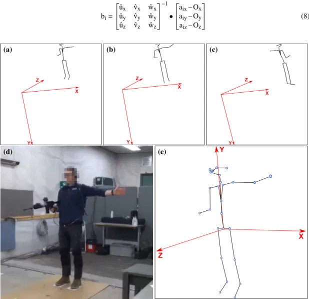
Because the raw data from the three Kinect sensors were expressed in their own absolute cartesian coordinate system with the origin located at the sensor’s position (Figure 5 (a-c)), some pre-processing was required. The first steps involved matching the raw data from the three devices both temporally and spatially, and to isolate the body of interest, i.e. the shooter. We used a body-centric coordinate system, as suggested by Vemulapalli et al. (2014). The synchronisation movement performed by the participant was used to synchronise sensor data temporally, and as a frame of reference for calculating new basis vectors. The synchronisation skeleton frame (S) and the following ten time frames (roughly 0.33 seconds) were used to calculate the new basis vectors, from which transformation matrices were constructed for each sensor device’s skeleton data. The normalised basis vector ˆu (representing the new X axis) was defined as the average vector position between the left and right hip joints during the synchronisation sequence (Equation (1,2)). #»_{u =} S+10

∑

n

n

The normalised basis vector ˆv (representing the new Y axis) was defined as the average position of the vector formed from the spine-navel joint and the pelvis joint during the synchronisation sequence (Equation (3,4)). #»_{v =} S+10

∑

n

n

The basis vector ˆw (representing the new Z axis) was defined as the normalised cross product of the new X and Y axes (Equation (5,6)).

#»

w = #»u × #»v (5) _{w =ˆ} w#»

| #»w| (6)

The origin #»O used to translate coordinates to the new system was defined as the average pelvis joint position during the synchronisation sequence (Equation 7).

#» O = 1 N S+10

∑

n

Each joint vector #»a_ifrom the entire skeleton sequence was then transformed into#»b_iby computing the dot product of the translated joint position and the change-of-basis matrix. The change-of-basis matrix was constructed by appending the columns of the three basis vectors and taking the inverse of the resulting matrix (Equation 8). b_i=   ˆux ˆvx wˆx ˆu_y ˆv_y wˆy ˆu_z ˆv_z wˆz   –1 •   a_ix– Ox a_iy– O_y a_iz– Oz   (8) Z X Y (a) (a) (a) (a) (a) (a) (a) (a) (a) (a) (a) (a) (a) (a) (a) (a) (a) (a) (a) (a) (a) (a) (a) (a) (a) (a) (a) (a) (a) (a) (a) (a) (a) (a) (a) (a) (a) (a) (a) (a) (a) (a) (a) (a) (a) (a) (a) (a) (a) (a) (a) (a) (a) (a) (a) (a) (a) (a) (a) (a) (a) (a) (a) (a) (a) (a) (a) (a) (a) (a) (a) (a) (a) (a) (a) (a) (a) (a) (a) (a) (a) (a) (a) (a) (a) (a) (a) (a) (a) (a) (a) (a) (a) (a) (a) (a) (a) (a) (a) (a) (a) (a) (a) (a) (a) (a) (a) (a) (a) (a) (a) (a) (a) (a) (a) (a) (a) (a) (a) (a) (a) (a) (a) (a) (a) (a) (a) (a) (a) (a) (a) (a) (a) (a) (a) (a) (a) (a) (a) (a) (a) (a) (a) (a) (a) (a) (a) (a) (a) (a) (a) (a) (a) (a) (a) (a) (a) (a) (a) (a) (a) (a) (a) (a) (a) (a) (a) (a) (a) (a) (a) (a) (a) (a) (a) (a) (a) (a) (a) (a) (a) (a) (a) (a) (a) (a) (a) (a) (a) (a) (a) (a) (a) (a) (a) (a) (a) (a) (a) (a) (a) (a) (a) (a) (a) (a) (a) (a) (a) (a) (a) (a) (a) (a) (a) (a) (a) (a) (a) (a) (a) (a) (a) (a) (a) (a) (a) (a) (a)(a)(a)(a)(a)(a)(a)(a)(a)(a)(a)(a)(a)(a)(a)(a)(a)(a)(a)(a)(a)(a)(a)(a)(a)(a)(a)(a)(a)

Y Z X (b) (b) (b) (b) (b) (b)(b)(b)(b)(b)(b)(b)(b)(b)(b)(b)(b)(b)(b)(b)(b)(b)(b)(b)(b)(b)(b)(b)(b)(b)(b)(b)(b)(b)(b)(b)(b)(b)(b)(b)(b)(b)(b)(b)(b)(b)(b)(b)(b)(b)(b)(b)(b)(b)(b)(b)(b)(b)(b)(b)(b)(b)(b)(b)(b)(b)(b)(b)(b)(b)(b)(b)(b)(b)(b)(b)(b)(b)(b)(b)(b)(b)(b)(b)(b)(b)(b)(b)(b)(b)(b)(b)(b)(b)(b)(b)(b)(b)(b)(b)(b)(b)(b)(b)(b)(b)(b)(b)(b)(b)(b)(b)(b)(b)(b)(b)(b)(b)(b)(b)(b)(b)(b) (b) (b) (b) (b) (b) (b) (b) (b) (b) (b) (b) (b) (b) (b) (b) (b) (b) (b) (b) (b) (b) (b) (b) (b) (b) (b) (b) (b) (b) (b) (b) (b) (b) (b) (b) (b) (b) (b) (b) (b) (b) (b) (b) (b) (b) (b) (b) (b) (b) (b) (b) (b) (b) (b) (b) (b) (b) (b) (b) (b) (b) (b) (b) (b) (b) (b) (b) (b) (b) (b) (b) (b) (b) (b) (b) (b) (b) (b) (b) (b) (b) (b) (b) (b) (b) (b) (b) (b) (b) (b) (b) (b) (b) (b) (b) (b) (b) (b) (b) (b) (b) (b) (b) (b) (b) (b) (b) (b) (b) (b) (b) (b) (b) (b) (b) (b) (b) (b) (b) (b) (b) (b) (b) (b) (b) (b) (b) (b) (b) (b) (b) (b) (b) (b) Z X Y (c) (c) (c) (c) (c) (c) (c) (c) (c) (c) (c) (c) (c) (c) (c) (c) (c) (c) (c) (c) (c) (c) (c) (c) (c) (c) (c) (c) (c) (c) (c) (c) (c) (c) (c) (c) (c) (c) (c) (c) (c) (c) (c) (c)(c)(c)(c)(c)(c)(c)(c)(c)(c)(c)(c)(c)(c)(c)(c)(c)(c)(c)(c)(c)(c)(c)(c)(c)(c)(c)(c)(c)(c)(c)(c)(c)(c)(c)(c)(c)(c)(c)(c)(c)(c) (c) (c) (c) (c) (c) (c) (c) (c) (c) (c) (c) (c) (c) (c) (c) (c) (c) (c) (c) (c) (c) (c) (c) (c) (c) (c) (c) (c) (c) (c) (c) (c) (c) (c) (c) (c) (c) (c) (c) (c) (c) (c) (c) (c) (c) (c) (c) (c) (c) (c) (c) (c) (c) (c) (c) (c) (c) (c) (c) (c) (c) (c) (c) (c) (c) (c) (c) (c) (c) (c) (c) (c) (c) (c) (c) (c) (c) (c) (c) (c) (c) (c) (c) (c) (c) (c) (c) (c) (c) (c) (c) (c) (c) (c) (c) (c) (c) (c) (c) (c) (c) (c) (c) (c) (c) (c) (c) (c) (c) (c) (c) (c) (c) (c) (c) (c) (c) (c) (c) (c) (c) (c) (c) (c) (c) (c) (c) (c) (c) (c) (c) (c) (c)(c)(c)(c)(c)(c)(c)(c)(c)(c)(c)(c)(c)(c)(c)(c)(c)(c)(c)(c)(c)(c)(c)(c)(c)(c)(c)(c)(c)(c)(c)(c)(c)(c)(c)(c)(c)(c)(c)(c) (d) (d) (d) (d) (d) (d) (d) (d) (d) (d) (d) (d) (d) (d) (d) (d) (d) (d) (d) (d) (d) (d) (d) (d) (d) (d) (d) (d) (d) (d) (d) (d) (d) (d) (d) (d) (d) (d) (d) (d) (d) (d) (d) (d) (d) (d) (d) (d) (d) (d) (d) (d) (d) (d) (d) (d) (d) (d) (d) (d) (d) (d) (d) (d) (d) (d) (d) (d) (d) (d) (d) (d) (d) (d) (d) (d) (d) (d) (d) (d) (d) (d) (d) (d) (d) (d) (d) (d) (d) (d) (d) (d) (d) (d) (d) (d) (d) (d) (d) (d) (d) (d) (d) (d) (d) (d) (d) (d) (d) (d) (d) (d) (d) (d) (d) (d) (d) (d) (d) (d) (d) (d) (d) (d) (d) (d) (d) (d) (d) (d) (d) (d) (d) (d) (d) (d) (d) (d) (d) (d) (d) (d) (d) (d) (d) (d) (d) (d) (d) (d) (d) (d) (d) (d) (d) (d) (d) (d) (d) (d) (d) (d) (d) (d) (d) (d) (d) (d) (d) (d) (d) (d) (d) (d) (d) (d) (d) (d) (d) (d) (d) (d) (d) (d) (d) (d) (d) (d) (d) (d) (d) (d) (d) (d) (d) (d) (d) (d) (d) (d) (d) (d) (d) (d) (d) (d) (d) (d) (d) (d) (d) (d) (d) (d) (d) (d) (d) (d) (d) (d) (d) (d) (d) (d) (d) (d) (d) (d) (d) (d) (d) (d) (d)(d)(d)(d)(d)(d)(d)(d)(d)(d)(d)(d)(d)(d)(d)(d)(d)(d)(d)(d)(d)(d)(d)(d)(d) Z X Y (e) (e) (e) (e) (e) (e) (e) (e) (e) (e) (e) (e) (e) (e) (e) (e) (e) (e) (e) (e) (e) (e) (e) (e) (e) (e) (e) (e) (e) (e) (e) (e) (e) (e) (e) (e) (e) (e) (e) (e) (e) (e) (e) (e) (e) (e) (e) (e) (e) (e) (e) (e) (e) (e) (e) (e) (e) (e) (e) (e) (e) (e) (e) (e) (e) (e) (e) (e) (e) (e) (e) (e) (e) (e) (e) (e) (e) (e) (e) (e) (e) (e) (e) (e) (e) (e) (e) (e) (e) (e) (e) (e) (e) (e) (e) (e) (e) (e) (e) (e) (e) (e) (e) (e) (e) (e) (e) (e) (e) (e) (e) (e) (e) (e) (e) (e) (e) (e) (e) (e) (e) (e) (e) (e) (e) (e) (e) (e) (e) (e) (e) (e) (e) (e) (e) (e) (e) (e) (e) (e) (e) (e) (e) (e) (e) (e) (e) (e) (e) (e) (e) (e) (e) (e) (e) (e) (e) (e) (e) (e) (e) (e) (e) (e) (e) (e) (e) (e) (e) (e) (e) (e) (e) (e) (e) (e) (e) (e) (e) (e) (e) (e) (e) (e) (e) (e) (e) (e) (e) (e) (e) (e) (e) (e) (e) (e) (e) (e) (e) (e) (e) (e) (e) (e) (e) (e) (e) (e) (e) (e) (e) (e) (e) (e) (e) (e) (e) (e) (e) (e) (e) (e) (e) (e) (e) (e) (e) (e) (e) (e) (e) (e) (e) (e) (e) (e) (e) (e) (e) (e) (e) (e)(e)(e)(e)(e)(e)(e)(e)(e)(e)(e)(e)(e)(e)(e)(e)

Figure 5. Skeleton synchronisation and merging.

(a-c): A participant performing the synchronisation movement from the views of the front left (a), front right (b), and back (c) sensors, with the origins of their coordinate systems at the sensor positions.

(d): A captured frame of the participant from the view of the front left sensor.

(e): The merged version of the sensors, with the coordinate system aligned with the body positions.

Despite the sensor data being transformed into the same coordinate system, the joint estimations and body rotations from the three sensors differed slightly, which made skeleton merging difficult. To overcome this, we used the sensor on the side of the weapon-holding hand as a reference, and attached body-centric joint positions from the other sensors to this sensor’s skeleton. These joint positions were calculated by performing new body-centric transformations on each skeleton frame for each sensor, ensuring that the body orientation was not affected by the differing sensor estimations. We then computed the average position c_i for each joint having a high confidence value (i.e. not occluded by other body parts), and transformed and translated it into d_i, represented in the coordinate system of the sensor on the side of the

weapon-holding hand with the originO and change-of-basis matrix [ˆu, ˆv, ˆ#» w] (Equation 9). d_i=     ˆu_x ˆv_x wˆ_x ˆu_y ˆv_y wˆ_y ˆu_z ˆv_z wˆ_z  •   c_ix c_iy c_iz    +   O_x O_y O_z   (9)

Although we used three sensors to prevent the occlusion of body parts, joints were sometimes out of view from any of the sensors, resulting in outlier positions. To simulate the actual trajectory of these joints, we estimated their positions with a loosely fit 4th degree polynomial regression from the surrounding high confidence frames. To remove twitching joint movements, we performed a median smoothing on each frame from the surrounding five frames, followed by a mean smoothing from the surrounding three frames, resulting in a smooth merged skeleton representation (Figure 5e).

We used the microphone sensor on our portable sensor platform to detect shots. The shot times and hit positions detected by the external LOMAH shot detection system could then be matched to these shots, and in turn to our skeleton and weapon sensor data.

From the merged skeletons, we extracted features based on the angles of bones formed by the vectors between connected joints (e.g. the right femur bone between the right hip and knee [Appendix A]). This representation retained most of the information in the data, but made it invariant of the absolute position of the body in a coordinate system, allowing the model training on the data to focus on finding relevant patterns. The angle values for a bone were represented in three radian values defined by the angle value of the bone against the X, Y, and Z basis vector respectively (Figure 6).

Right femur bone feature representation: [0.44, 1.11, 2.33]

1.11 rad 0.44 rad 2.33 rad Z X Y

Figure 6. Skeleton bone feature representation. Each bone was defined by three features per frame (X, Y, and Z angles), here illustrated for the right femur bone from a frame in a skeleton sequence.

To make the models more robust, we used a set of data augmentations: For each skeleton sequence, six new orientations were produced from rotations around the Y axis with 10◦, 20◦, and 40◦rotation to both the left and the right, and used to train the model in addition to the original orientation, as suggested by N´u˜nez et al. (2018). During model training, we also added Gaussian noise randomly to some of the bone features in an attempt to make the models more robust to imperfect data.

6.2

Feature embedding and ViT adaptation

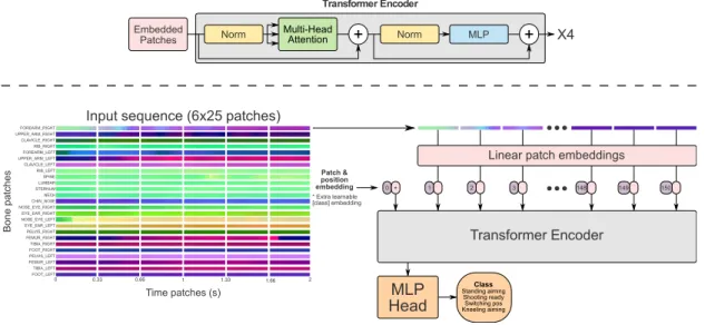
Because of the strength of Transformers on sequential data tasks, as well as their inherent explainability capabilities, we chose a Vision Transformer (ViT) (Dosovitskiy et al., 2021) for our tasks. We represented each skeleton sequence with time frames as columns, and the 25 different bones as rows with the X, Y, and Z radian values stacked on each other. We used a fixed feature representation of 3x25x60 scalar values, i.e. a skeleton sequence of two seconds with 30 frames per second, and embedded this into patches of size 3x1x10. This meant that each patch represented one bone and its radian X, Y, and Z components over a time period of roughly one third of a second (Figure 7). The feature representation was partly inspired by Ke et al. (2017), who divided their data into time clips consisting of separated cylindrical coordinates. Because our patches were one row in height, representing only one bone, each bone for a moment of time could attend to any bone and time (including itself) across the patch embeddings. This allowed us to extract the attention for each bone and sub-sequence for a prediction, explaining some of the model’s reasoning. The ViT model used four multi-head attention layers composed of eight heads for each layer. A multilayer perceptron (MLP) head attached at the end of the model produced the output(s) for the specific task (Figure 7). Each attention layer used a Gaussian Error Linear Unit (GELU) activation function. For both our learning tasks, we used a dropout of 0.3, as well as a reduce-on-plateau learning rate starting on 1x10–3, and reducing by a factor of 0.3 after plateauing for three epochs. See Appendix B for all model parameters.

0 0.33 0.66 1 1.33 1.66 2

Time patches (s)

Input sequence (6x25 patches) FOREARM_RIGHT UPPER_ARM_RIGHT CLAVICLE_RIGHT RIB_RIGHT FOREARM_LEFT UPPER_ARM_LEFT CLAVICLE_LEFT RIB_LEFT SPINE LUMBAR STERNUM NECK CHIN_NOSE NOSE_EYE_RIGHT EYE_EAR_RIGHT NOSE_EYE_LEFT EYE_EAR_LEFT PELVIS_RIGHT FEMUR_RIGHT TIBIA_RIGHT FOOT_RIGHT PELVIS_LEFT FEMUR_LEFT TIBIA_LEFT FOOT_LEFT Bone pa tches

Linear patch embeddings

1 2 3 148 149 150 0 Transformer Encoder Transformer Encoder Embedded Patches + X4 * MLP Head Class Standing aiming Shooting ready Switching pos Kneeling aiming Multi-Head Attention + Patch & position embedding * Extra learnable [class] embedding Norm Norm MLP

Figure 7. Model architecture. The input patches produced from a skeleton sequence, and how they were processed by the ViT model. Adapted from Dosovitskiy et al. (2021).

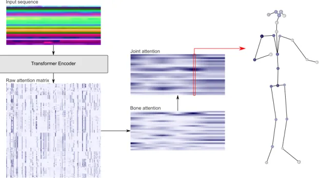
For each prediction, the model produced 32 attention matrices from the eight heads of the four attention layers, which we summed up into one representation of the attention. Figure 8 shows how the attention map was processed from the raw attention map produced by the model into a format that we deemed easier for humans to interpret, explaining which joints affected the prediction for each time frame.

6.3

Shooting pose estimation

Estimating the pose of a shooter in a shooting scenario could be useful in a live prediction situation in a larger system. Such a system could potentially be made up of many different models trained for judging different shooting poses, and would therefore need some way of determining the current shooting pose. The pose classification task was used for demonstrating the capabilities of the workflow presented in this thesis. We identified and labelled four pose classes from the data collection scenario: standing shooting ready, standing aiming, switching position, and kneeling shooting. The labels were automatically assigned based on the timing of shots. We labelled the frames as standing or kneeling aimingfrom 0.5 seconds before the first shot of a 3-shot sequence to the last shot of that sequence.

Transformer Encoder Input sequence

Raw attention matrix

Bone attention Joint attention

Figure 8. Attention extraction. Pipeline describing the process from an input skeleton sequence to an explainable attention visualisation for a model prediction.

Each 60 frames (two second) long skeleton sequence belonging entirely to one class label was extracted from the scenario. New sequences were extracted starting at every third frame. For this learning task we used a cross entropy loss over four output nodes for our four classes, and a batch size of 256 samples. Because the classes were not equally distributed (Table 1), we used an imbalanced class data sampler to semi-randomly upsample the classes with few samples, and downsample the classes with many samples during training. We separated the 13 participants into folds in a 13-fold cross validation. This ensured that the model did not overfit to one specific participant during training. For each fold, we used one participant for testing, 10 participants for training, and two participants for validation. The training participant samples were fully augmented as described in the Data pre-processing section.

Table 1

Class distribution for the pose estimation task.

Pose class Samples % of distribution

Standing shooting ready 6,976 43.39

Standing aiming 2,329 14.48

Switching position 1,864 11.59

Kneeling aiming 4,910 30.54

6.4

Shooting performance estimation

To predict the performance of shooters, we modelled a regression task with a continuous shooting score as the target, and a skeleton sequence of two seconds as the input. We used the same feature representation as in the pose estimation task, and the same model architecture apart from a smaller batch size of 64 samples, as well as one output value with a mean squared error loss function. Hoping to transfer some knowledge from the pose estimation task, we used a parameter transfer from the trained pose models to this task. Because we were limited by using a fixed input size, we predicted the score of each shot separately. The shooting score target variable was calculated using the euclidean distance from the centre cross of the target (Figure 3b). This score ranged from 10 points for a centre hit, linearly decreasing out to 20 centimetres from the centre, and 0 points from 20 centimetres and outwards. This score was then

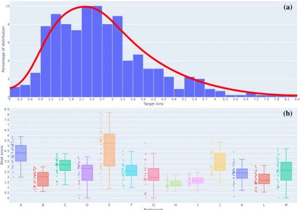
divided with the time taken for each 3-shot series, as the shooters were instructed to perform the scenario with both speed and accuracy. Dividing the score with the time taken improved the distribution of the regression target, although the data was slightly skewed towards the lower part of the interval (Figure 9a). For easier interpretation, we scaled this target variable to range between zero and one by dividing them with the top score for a shot (8.17). To limit the scope of this task, we only looked at standing shots, meaning that for each participant, we extracted six skeleton sequences for each of their six scenarios. Some scenarios were excluded due to poor sensor readings, however, resulting in a final number of 449 samples. We performed the same 13-fold cross validation as in the pose estimation task.

0 0.3 0.6 0.9 1.2 1.5 1.8 2.1 2.4 2.7 3 3.3 3.6 3.9 4.2 4.5 4.8 5.1 5.4 5.7 6 6.3 6.6 6.9 7.2 7.5 7.8 8.1 8.4 0 2 4 6 8 10 Target bins Perce ntage of dis tribu tion (a) A B C D E F G H I J K L M 0 0.5 1 1.5 2 2.5 3 3.5 4 4.5 5 5.5 6 6.5 7 7.5 8 8.5 Participant Shot score (b)

Figure 9. Regression target distribution.

(a): The curve distribution of our shot score regression target variable. (b): The score distribution of the shots of each individual participant.

7

Results and analysis

7.1

Pose estimation

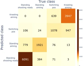
The results from the pose estimation task are shown in a confusion matrix in Figure 10. Because our class distribution was imbalanced, we used both Accuracy and Cohen’s κ as evaluation metrics, as Accuracy would be biased towards majority classes, whereas Cohen’s κ measures how much the prediction was than a random prediction given the class distributions (Sim & Wright, 2005). We computed both the total result metrics and the 95% confidence intervals based on the results from each fold (participant) in the experiment (Figure 11). It is worth noting that the confidence intervals were computed with unequal fold sizes; the participant with the most samples had 1792 samples, whereas the one with the fewest samples had only 815 samples. The model performed best on standing shooting ready and kneeling aiming, but often confused switching position with kneeling aiming, as well as standing aiming with standing shooting readyto some extent. These were reasonable errors, as these were the classes most similar to each other. In addition to this, the labelling was not always correct.

Standing shooting ready Standing aiming Switching pos Kneeling aiming Standing aiming 0 1000 2000 3000 4000 5000 6000 True class Predic ted cl ass 6091 384 71 3 779 1921 76 13 106 24 1078 947 0 0 639 3947 Standing shooting ready Switching pos Kneeling aiming

Figure 10. Confusion matrix. True and false positives and negatives for the results of the pose estimation task.

Cohen's κ Total Cohen's κ

CI 95% AccuracyCI 95% AccuracyTotal

Score 0.9 1 0.8 0.7 0.6 0.5 0.4 0.3 0.2 0.1 0 0.73 0.81 0.66 0.77 0.77 0.85

Figure 11. Pose estimation metrics. Total Cohen’s κ and Accuracy metrics, as well as 95 % confidence intervals. The confidence intervals were computed from the metrics from the 13 folds in the cross validation.

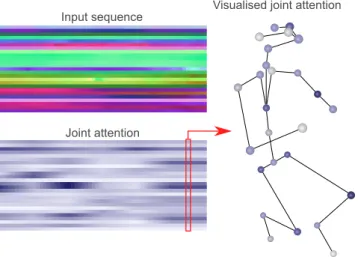
Figure 12 and Figure 13 show visualisations of the processed attention produced from the model. The attention often focused on the position of one of the femur bones, which was reasonable, as the angle of this bone could help the model determine whether a target was standing or kneeling. Figure 12 (switching position) highlights the fact that the model attended to the left femur bone in the visualised time frame, but also earlier in the sequence when the participant was in a standing position. This indicates that the model has learned to attend to the changing angle of the femur bones to determine whether the sequence involved switching from a standing to a kneeling position or not. Figure 13 (standing aiming) shows that the model attended a lot to both femur bones, as well as the shoulder and upper arm of the dominant shooting hand, indicating that the model attends to relevant features.

Input sequence

Joint attention

Visualised joint attention

Figure 12. Attention visualisation: Switching position. The input skeleton sequence of one of the participant switching from a standing to a kneeling position, the joint attention produced from the attention matrix from the pose estimation model, and a skeleton visualisation of the joint attentions for one time frame. Darker colour indicates stronger attention.

Input sequence

Joint attention

Visualised joint attention

Figure 13. Attention visualisation: Standing aiming. The input skeleton sequence of one of the participant standing and aiming, the joint attention produced from the attention matrix from the pose estimation model, and a skeleton visualisation of the joint attentions for one time frame. Darker colour indicates stronger attention.

Because of our high accuracy of 0.81 on an imbalanced class task, as well as a Cohen’s κ score of 0.73 (which is a substantial result for this metric (Landis & Koch, 1977)), our first hypothesis: It is possible to separate the different phases of a rifle shooting scenario with body tracking data, has been confirmed by the experiment.

7.2

Shooting performance estimation

The results and metrics from the regression experiment can be seen in Figure 14(a,b). We evaluated the results using mean absolute error and root mean squared error from the ground truth, as well as the 95% confidence interval between the participant folds. The standard deviation of the regression targets was 0.172, which was close to our evaluation metrics, meaning results were only very slightly better than completely random predictions. The regression plot (Figure 14a) also highlights that no discernible pattern could be found in the model’s predictions. Ideally the predictions should follow a similar curve to the targets, but the rolling average of the predictions did not follow the target curve at all, forming close to a horizontal line. 0 50 100 150 200 250 300 350 400 450 0 0.2 0.4 0.6 0.8 1 Target Prediction

Rolling prediction average

Sample Shooting score (a) 0.10 0.15 0.20 0.25 0.30 0.35 0.40 0.45 0.50 MAE

CI 95% MAETotal CI 95%RMSE RMSETotal 0.12 0.19 0.16

Error

Figure 14. Shooting performance estimation metrics.

(a): The regression target and prediction plots for the regression model, sorted by target value. The vertical bars represent the absolute error of each sample. The faded red line represents a rolling average of the predictions of the closest 30 samples.

(b): Total Mean Absolute Error (MAE) and Root Mean Squared Error (RMSE) metrics, as well as 95 % confidence intervals for the regression model. The confidence intervals were computed from the metrics from the 13 folds in the cross validation.

The second hypothesis: There is a correlation between body postures as measured by body tracking sensors, and rifle shooting performance,could neither be confirmed nor rejected by our experiments. We were not able to show any statistically significant correlation from our data, but we also could not reject the idea that there is a correlation between body movements and rifle shooting performance.

8

Discussion

Using three Kinect sensors to limit the poor pose estimations caused by occluded body parts worked to an extent. However, joints were still sometimes occluded, and would occasionally stutter substantially between frames. This may have limited the possibilities for our model to detect finer movement details. There is a possibility that the joint positions produced by the Kinect sensors were simply too low quality to be used to accurately estimate shooting performance. Kneeling or sitting postures led to very poor joint estimations, and the Kinect could almost never accurately represent crossed legs. Standing poses, however, were generally represented better. Using the joint estimation confidence produced by the Kinect as a way of detecting incorrect joint positions worked well. Interpolation through polynomial regression of the surrounding high-confidence frames served as a good heuristic for the actual joint positions for these frames, making the skeletons represent reality better. Median and mean smoothing helped reduce jitter by removing the joint outliers that still remained after the interpolation, which also led to better skeleton visualisations. Because these smoothing techniques risked damaging information relevant for making correct predictions, only minor adjustments were made. However, it is possible that they affected the final results.

The synchronisation movement helped us match the three sensors’ skeleton data temporally and spatially, although poor sensor readings made it difficult to perform a perfect matching. Despite transforming the different sensor data to the same coordinate system, their differences in intra-skeleton joint estimations was an additional issue for skeleton merging; one sensor could estimate the hand to be slightly further away from the other joints of the body than another sensor, and in a slightly different relative direction. Performing a transformation on each single frame helped to circumvent these issues. The use of a microphone sensor to detect shots on the portable platform and match them with the external LOMAH shots worked well overall. Although we failed to match some shots between the two devices, roughly 96% of the collected data could be used in the experiments.

Some compromises were made in the selection of participants due to safety constraints, both in the number of participants and the amount of scenarios they could perform. Ideally there would have been a wide variety of skill levels represented among the participants. Having half the scenarios be performed with the non-dominant shooting hand to simulate different skill levels seemed to work to some extent; shooters shot better and faster with their dominant hand, and their body postures and movements were generally more in line with shooting doctrine.

Shooting performance could not be correlated to our body tracking data. This could be due to many different factors, such as poor sensor readings, or the dataset being too small and not diverse enough. Additionally, body postures in general may not have a large enough effect on shooting performance to be used as a sole factor; many other factors such as trigger jerking, small weapon movements, and eye movements could potentially have a larger impact on performance (Ball et al., 2003). There have also been conflicting reports on whether postural stability correlates to shooting performance across multiple individuals (Ball et al., 2003; Era et al., 1996). Various shooting styles were observed from the participants; some had a very forward leaning, aggressive shooting pose, whereas others had a more upright pose while still achieving high scores. With only 13 participants, these differences in body postures may have been detrimental to the discriminative powers of our model. Time was not included as a factor in the input of our skeleton sequences because we judged that this could cause the model to only attend to the time aspect, and ignore postural features. However, time was included as a factor in our score calculations to produce a more diverse regression target distribution (Figure 9a). This was potentially negative for our model, because a faster shooter may not have better posture than a slower one. Ideally, the regression should have been normally distributed. However, Figure 9a highlights a skewing towards the lower part of the interval for our target.

The pose estimation task saw stronger performance (Figure 11), likely due to the larger differences in poses compared to the shooting performance estimation task. The confusion matrix (Figure 10) indicates that the model has learned a reasonable representation, as the poses that were classified incorrectly were usually the most similar to each other. Because the pose labelling was performed automatically by using shot moments, the labels were not always accurate. All frames up until 0.5 seconds before the first

kneeling shot were labelled as belonging to the switching position class. However, many participants spent a significantly longer time after switching position before firing their first shot, meaning that more frames should have been labelled as kneeling aiming. Many of the standing shots were also incorrectly labelled, as many participants continued to aim for some time after firing their first standing shots instead of moving to a shooting ready position with the weapon aimed down. Some participants also aimed for more than 0.5 seconds when standing up before firing their first shot. Using a combination of up- and downsampling seems to have removed any bias towards majority classes (Figure 10), despite the largest class having roughly four times more samples than the smallest class (Table 1). Taking into account the incorrect labels and the class imbalance, the model can be judged to have performed quite well. Manual study of the samples and attentions indicates that it has learned to look mostly at correct factors for discriminating between the classes.

A limiting factor to our transformer model was the fixed input size, i.e. all bones and their radian X, Y, and Z values over a sequence of 60 time frames (two seconds). Using longer sequences would require aggregating the data along the time dimension, which would cause the model to perceive subjects to be moving much faster than they were in reality. A potential workaround to this would be to include a time token in the input sequence, indicating to the model that it should judge samples differently based on time taken. Although standard transformer models could use different input sizes, we speculate that longer sequences would be more difficult to train on, and thus require more data. Other sequential models such as LSTMs, or GCNs using graphs across time could work well for the learning tasks, but would not produce the same level of explainability.

The attention mechanism produced explainable predictions from our models, often being able to attend to the relevant frames and bones, as was also observed by Song et al. (2017) and Plizzari et al. (2020). We only focused on explaining predictions from the pose estimation model, as the explanations were deemed to be useless if the model did not perform well. When the predictions had high confidence, the attention generally highlighted relevant factors for the predicted pose. With poor prediction confidence, however, it was often more difficult to interpret the attention. Figure 12 and Figure 13 show how a frame from a prediction could be explained through visualisation by colouring the joints of a skeleton frame with the values from a processed attention matrix. Longer sequences were visualised using 3D modelling or videos of skeletons with continuously shifting levels of attention on joints. In our opinion, the visualisation provides an intuitive insight into the model’s reasoning, which can aid both in better model development, and as a basis for decision making during rifle shooting training.

Our research question was:

Can relevant factors for rifle shooting tasks be determined through posture and body movements? We argue that relevant factors have been extracted to some extent; we have separated the phases of our shooting scenario solely through body tracking data. We also managed to determine relevant factors that contributed to predictions through the attention mechanism. However, we were unable to correlate shooting performance to our data.

8.1

Future work

Although we have shown how data collection could be planned and performed, how sensors could be synchronised, merged, and processed, and how the resulting data could be used in explainable machine learning tasks, there are many possibilities for future studies. For better shooting performance estimation, there may be a need for more manual features based on expert knowledge of the shooting domain, such as mean sway velocity and other established factors (Aalto et al., 1990; Era et al., 1996; Mononen et al., 2007). Although deep learning models can generally find important features from raw data, our relatively small dataset could benefit from handcrafted features with more discriminative power. Such features could be used both in classical machine learning models or as additional dimensions in the architecture proposed in this thesis. Another future step could be to examine different regression target sampling techniques for a better target distribution than the one presented in Figure 9a. Different input sequence lengths would allow for studying both long- and short-term movement patterns. This could be done by warping inputs of different lengths to one size and including some time indication token, or through using multiple models with different input sizes, or models capable of dealing with varying input sizes.