Optimal Cooperative Platooning Using Micro-Transactions

(1)

(2)

Optimal Cooperative Platooning using Micro-Transactions

Philip Ahl

Supervisor(s):

Doctor Henrik Svärd, NCPP, Scania Senior Engineer Svante Johansson, NCPP, Scania

Subject reader:

Professor Alexander Medvedev, Department of Information Technology, Uppsala University Examiner:

Docent Tomas Nyberg, Department of Electrical Engineering, Uppsala University

Master of Science Thesis in Engineering Physics, Embedded Systems Department of Engineering Sciences, Uppsala University, Sweden 2020

In collaboration with Scania CV AB, Södertälje August 5, 2020

(3)

Teknisk- naturvetenskaplig fakultet UTH-enheten Besöksadress: Ångströmlaboratoriet Lägerhyddsvägen 1 Hus 4, Plan 0 Postadress: Box 536 751 21 Uppsala Telefon: 018 – 471 30 03 Telefax: 018 – 471 30 00 Hemsida: http://www.teknat.uu.se/student

Abstract

Optimal Cooperative Platooning Using

Micro-Transactions

Philip Ahl

The urge to consume do not seem to stop, thus, the need for transportation of goods will most likely not decrease. At the same time jurisdictions and regulations around green house gas emissions are sharpening and pushing the industry towards a more

environmentally friendly state. The freight and transportation industry is facing a huge challenge in the upcoming years and solutions are needed to feed the demand of society.

Two, of many, proposals of solving, at least, parts of the above mentioned problem is platooning and the look-ahead controller. Platooning denotes the concept of slipstream where maximum utilization of aerodynamic drag reduction is endeavoured. The look-ahead controller exploits the surrounding topographical information in order to yield an optimal driving strategy, often resulting in that the vehicle initiates the phenomenon of pulse and glide, which denotes alternating between high load operation points and freewheeling, i.e. engaging neutral gear.

This work have sought to investigate these concepts to determine whether or not additional fuel-efficiency can be added by

manipulating and re-designing the control unit of the system. The proposed addition is built upon the look-ahead controller and supplements it by enabling communication between vehicles such that micro-transactions may occur in order to aid decision making

regarding the choice of driving strategies.

A vehicle model, a platoon model and the novel optimization based look-ahead-controller was synthesized and developed, where dynamic programming was used as the optimization solver of the controller. The look-ahead controller was verified such that one can conclude that it behaves according to the assumptions of such a system. The proposed micro-transaction system was also verified to conclude that it behaves as assumed, yielding a reduction in fuel consumption. For a platoon of two members, a 1.2% and 1.7% reduction in fuel consumption for the leading and following vehicle respectively was obtained, compared to an identical platooning setup, using a look-ahead controller, but where no negotiations using micro-transactions are allowed between the vehicles.

Ämnesgranskare: Alexander Medvedev Handledare: Henrik Svärd & Svante Johansson

(4)

1 Populärvetenskaplig sammanfattning

Drivet av samhället att konsumera mer verkar inte avta, således lär inte behovet av att transportera varor och tjänster avta. Parallellt med utvecklingen av våra behov stramas regler och lagar åt kring växthusgaser, vilket pressar industrin mot ett miljövänligare tillstånd. Transportindustin kommer därmed att möta stora utmaningar de kommande åren för att mätta samhällets konstant växande och hungrande begär.

Två, av många, förslag på att lösa, åtminstone delar av, problemet som nämns ovan är konvojtåg och topografisk styrning. Konvojtåg benämner det koncept då man i rörlig linjeformation utnyttjar den luftström som bildas för att maximalt utnyttja de aerody-namiska fördelarna som tillkommer. En topografisk styrning utnyttjar informationen om den omgivande miljön runt fordonet för att kunna beräkna en optimal körstrategi givet den framtida kupering som fordonet kommer att möta, vilket ofta resulterar i att for-donet initierar ett pulserande beteende, då forfor-donet alternerar mellan att gasa i höga lastpunkter och frirulla i neutral växel.

Detta arbete strävar åt att undersöka dessa koncept för att avgöra huruvida ytterli-gare bränsleeffektivitet kan uppnås genom att manipulera och designa om styrningen av systemet. Den förslagna lösningen är byggt på den topografiska styrningen och tillför kommunikation mellan fordonen, så att mikrotransaktioner kan ske, för att assistera i beslutsfattande om körstrategier i konvojen.

En syntes av fordonsmodell och konvojmodell har ägt rum och en ny optimerings-baserad topografisk styrning har utvecklats, där dynamisk programmering har använts som optimeringslösare.

Den topografiska styrningen verifierades så att man kan dra slutsatsen att det beter sig som man kan anta att ett system av denna sort ska bete sig. Det förslagna mikro-transaktionssystemet verifierades också för att konkludera att det beter sig inom rim-liga ramar och en reduktion i bränslekonsumtion. För en konvoj på två medlemmar, uppmärksammades 1.2% samt 1.7% minskning i bränslekonsumption för det främre och bakre fordonet respektive, jämfört mot en identisk konvojinställning och omgivning, med den topografiska styrningen, men utan några förhandlande mikrotransaktioner mellan fordonen.

(5)

2 Acknowledgements

First and foremost, I thank my supervisors, Henrik Svärd and Svante Johansson, for be-ing helpful and guidbe-ing throughout this journey and for standbe-ing out with my relatively hideous implementations and hours of debugging. I would like to thank Viktor Leek and the NCPP departement at Scania for good coffee breaks and ever so weirdly interesting discussions. I thank Andreas Lycksam for making the lunch time a better hour of the day. I want to thank my friend David Sandberg, for moral support, and for the astonishing graphics on the front page.

I would also like to pay great respect to my dearest of friends, Nils, for constantly intellec-tually challenging me during our master and for all the good times we have had and will continue to have. I want to thank Lina, for always standing by my side and supporting me no matter the weather, and for standing out with my babbling about things that are relatively uninteresting for you. Last but absolutely not least, I want to thank my parents. For encouraging me to do the right thing at all times. To support me in such a wide spectrum throughout my education, for letting me eat up your fridge and for giving me roof over my head when needed. I literally and figuratively could not have done any of this without you.

(6)

3 Nomenclature

3.1 Abbreviations

Table 1: Useful abbreviations. Abbreviation Meaning

ACC Adaptive cruise control

ALAC Adaptive look-ahead control

BSFC Brake specific fuel-consumption

CACC Cooperative adaptive cruise control

CALAC Cooperative adaptive look-ahead control

CC Cruise control

DP Dynamic programming

ECU Electronic control unit

HDVs Heavy-duty vehicles

kWh kilo Watt hour

LAC Look-ahead control

LQG Linear-quadratic-Gaussian

MPC Model predictive control

MTC Micro-transaction Control

PnG Pulse and glide

(9)

3.2 Mathematical symbols

Table 2: Explanation of some mathematical symbols, in order of mention. Mathematical

symbol Meaning

u Control signal

U Set of all control signals

x State signal

X Set of all state signals

t Time tg time-gap j,k time index NM P C MPC horizon length f0 Cost function φ Weight function

O() Big O notation

P Power d dt Derivative operator W Work F Force m Mass v Velocity E Energy

g Gear, gravitational constant

M Torque

rw Wheel radius

A Frontal area of the vehicle

d Inter-vehicular distance

α Angle of the road slope

ω,ωwheel Angular velocity of the wheel

mf Fuel mass

J Cost-to-go

ξ Step-cost

ρd Density (diesel)

θd Energy density (diesel)

(10)

4 Introduction

Today we, as a species, are more concerned about our environmental impact than ever. This might be due to the increased communication capability, that information and cli-mate awareness is easily spread among us. Or it might stem from the fact that natural disasters such as tsunamis or forest fires are becoming more frequent and ever so demol-ishing and detrimental. As this concern increases, the list of reasons for being concerned becomes larger1_{, hence defining it as thorough as possible becomes harder and more time}

consuming. So leaving it as such, organisations and sectors all around the globe are trying to reduce their environmental footprint in the most profitable way as possible.

Road transportation plays a vital role in our modern society of consumerism. Goods of any kind needs to be transported from the producer to the costumer, with possible refineries and storaging on the way. In the European Union, almost 75% of the inland freight transportation is done by road which amounts to about a fifth of the human-related CO2 emissions, wherein heavy-duty vehicles (HDVs) amounts to about a fourth of that

share [1]. Due to the strong link between global economic growth and freight transporta-tion, the environmental impact of heavy-duty vehicles will grow, if no measures are taken. Although one might believe oneself not fully aware of the main concept of this thesis, pla-tooning, its presence may be more common than imagined. For example, when migrating birds are travelling to warmer latitudes for a season or when watching the peloton2 sprint

towards the finish line of the stage in le tour de France. Both these groups are exploit-ing the fact that drivexploit-ing (or flyexploit-ing for that matter) at short intermediate distances from each other reduces the energy spent on moving forward. This phenomenon is commonly known as the slipstream effect and can easily be generalised to most moving objects that are moving in a fluid which causes drag, such as air.

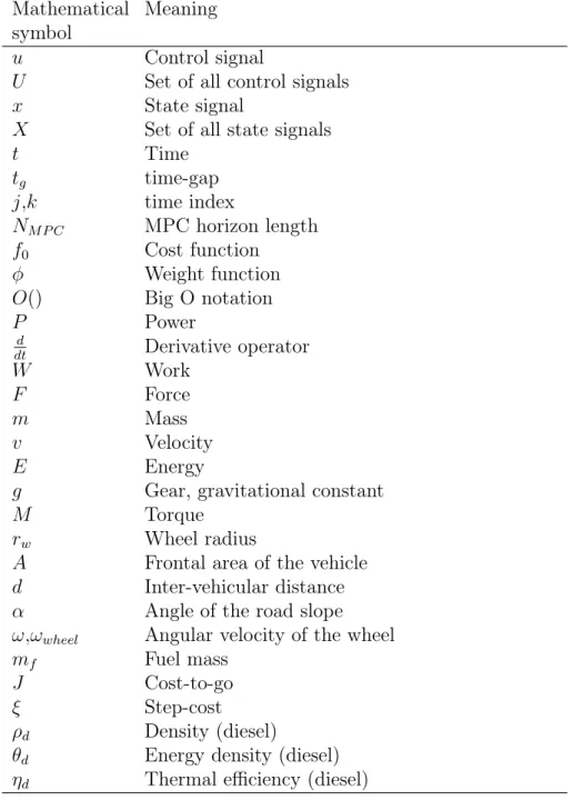
Integrating this technique with the existing heavy-duty transportation is a goal which would, if executed properly, increase the fuel-efficiency which would save fuel expendi-tures for the companies while leaving a smaller climate footprint, hence would kill two birds with one stone. This thesis aims at employing that integration in order to achieve better fuel-efficiency while maintaining safety by intelligently controlling HDVs in platoon formations, such as shown in Figure 1.

1_{Although the Intergovernmental Panel on Climate Change, IPCC, have boiled down the risks of}

climate change into a dense bouillon cube consisting of five reasons for concern, I mean that the reasons which reaches a daily personal basis, such as "it was so many years ago we had a snowy Christmas in Sweden"-reasons increases.

2_{Peloton means platoon in French and is commonly referred to a big group of road cyclists that}

(11)

Figure 1: Three-vehicle platoon driving 300 km above the Arctic Circle in Norway. [6]

4.1 Motivation

As the world’s population continuously grows and economies continues to expand, the demand of transporting goods is expected to increase. The International Transport forum predicts that for Economic Co-operation and Development countries the freight trans-portation, measured in tonne-kilometres, will increase between 40% and 125% and for developing countries an increase of up to 400% by 2050 compared to 2010 [2].

This large increase in goods transportation would mean great challenges for the in-dustries controlling and providing it with regard to energy consumption and emissions. Many involved countries signed the Kyoto protocol and more recently the Paris agreement to decrease emissions and waste of different kinds. In the European Union (EU), road transportation is responsible for 72% of the greenhouse gas emissions within all modes of transportation, whereas the transportation sector is the only one in the EU for which the greenhouse gas emissions are still rising [3].

Apart from the environmental effects on the climate and the responsibility for future generations, the surrounding environment is greatly affected as well. Air pollution is the number one environmental cause of death in the EU, leading to more than 400’000 premature deaths per year [4].

Apart from the environmental effects in general, a decrease in greenhouse gas emis-sions would imply an increase in fuel-efficiency, premised that the freight transportation is at least expanding. Increasing fuel-efficiency would be an economical benefit for the haulage companies for which fuel cost amounts for about 35% of the total costumer cost

(12)

in Europe [5].

Hence, given all this, it is not surprisingly that transportation solution providers are making a huge effort in developing fuel-efficient technologies. These efforts typically fo-cuses on optimization in the combustion engine and drivetrain, improved aerodynamics and tires or weight reduction but more recently the fuel-efficiency is altered through a more digital way using control systems. This thesis embraces this approach, aiming to fully explore the exploitation of its capacities, in order to add to the pond of knowledge and research, in which we are swimming, to find safe shore for ourselves and future selves.

4.2 The concept of platooning

The approaches to increase fuel-efficiency mentioned in Section 4.1 only focuses on one single vehicle. Additional benefits can be achieved if one enables cooperation between vehicles, whereas one approach will be of central importance in this thesis, namely pla-tooning.

Platooning or slipstreaming is the technique of exploiting the mass and area of each other with respect to air drag in order to reduce energy costs. Given a group that can communicate of at least two members, the one in the front is assumed to be the leader, directing the way forward. The leader creates a tunnel of air behind her with a lower relative speed with respect to the platooning members. This will reduce the air drag for the rear members increasingly as the distance between them reduces at the same time as it decreases for positions longer farther away from the leader in the formation. The frontal leader will also experience a slight reduction in air drag due to less adverse aerodynamic turbulence, not as significant as for the others but still noticeable [7].

This concept is highly used by professional cyclists, where they also use the direction of the current wind in order to optimize their topology such that the air resistance gets minimized. This aspect is not considered in this thesis, other limitations can be read in Chapter 4.5, Delimitations and challenges.

HDVs spend up to a forth of their fuel on overcoming the aerodynamic resistance [8], which makes it clear that reducing air drag for as many vehicles as possible would yield vast gains in fuel-efficiency. Apart from the fuel-efficient aspect, short inter-vehicular distances between transportation vehicles would increase the capacity of public roads, potentially decreasing traffic congestion.

Since human drivers would have difficulties in driving at as short inter-vehicular dis-tances as possible given the safety margins, which would be the optimal way to drive, it becomes obvious that automated driving systems are needed for such a task. Implement-ing a more automated drivImplement-ing technology would reduce the human error factor on public roads, which would also possibly result in decreasing road accidents where the human error factor is involved.

4.3 Problem formulation

The angle of which this work is attempting to solve the above mentioned in Chapter 4.1 is to investigate if and how a control system can aid to compensate for anomalies and

(13)

de-viations in a mutual optimal trajectory3_{. Can a modern control system, more precisely a}

Look-Ahead controller, be improved by enabling micro-transactions between the vehicles, in order for them to negotiate about changes in their planned optimal strategy?

The questions will be answered and tested through prototyping such a system, yielding a proof of concept more than a full product.

4.4 Thesis outline and contribution

The work in this thesis will be presented as follows. Chapter 4 will introduce the reader to the problem and briefly describe its orientation. Chapter 5 will provide the reader with background details in the technologies that this thesis will use and build upon. The chosen methodology of solving the optimization problem will be discussed and different modelling approaches that have been done by related research. Chapter 6 will explain the chosen model structure of this work. Derivations of the acting forces on the vehicle will lead up to the optimization problem statement. The Chapter ends with a motivation and conceptual description of the proposed micro-transaction controller. Chapter 7 will take the reader through how the control strategies were implemented and the verification of the control systems. Lastly Chapter 8 will be a discussion of the journey of this work and ideas of future work in the area.

The novel work that this thesis provides is the proposed micro-transaction control sys-tem, which will attempt to decentralize4 _{the platooning problem without the need of a}

platoon coordinator on top of the individual vehicle controllers.

4.5 Delimitations and challenges

If the technique of platooning is as promising as mentioned, one can ask the question why it is not yet implemented. The full answer might be deeply politically nested around concerns regarding infrastructure, safety and feasibility, but the following comments will be with disregard of political thresholds, focusing on the technical issues instead.

The impact of disturbances cannot be disregarded, but rather seen as the foremost resis-tance to the capability of a system of this sort. A lot of studies and research have been done in closed environments with small or no regard of external traffic have been allowed, e.g. by Alam et al. [11]. Few to none simulations, which is a major part in the research and development pipeline, have included it. Some experiments have been conducted on public roads but in order to gain the amount of data such that one can conclude diffi-culties and possible external constrains are yet to be done. This thesis will not include external traffic in its simulations, and does not have the intent to test its implementation on public roads, solely due to the limited time and computational resources for such a profound breadth.

3_{Throughout this work, the planned driving strategy, within the time-horizon of the problem, will}

often be denoted trajectory.

4_{Decentralized in this context means that all members using the proposed system will be able to}

work independently from any overview information source. Much like the federal laws of the US, where each state can decide its own laws (to some degree) apart from the Swedish system where the parliament governs each municipality. Thus, no hierarchic relations ought to be needed.

(14)

The external noise coming from fast and slow changes in weather and climate will not be addressed as well. Such fast changes could include wind or snow storms whilst the slow changes could include the geographical position with respect to the change in the gravitational constant when measuring the gravitational force.

Also, the fact that tires have an noticeable impact will be disregarded, where the different tire pressures, materials and patterns will not be altered. Hence the analysis and comparison will be seen with regard that these parameters are held constant. The scope of this thesis will be to simulate situations that the system will engage in, a proof of concept. Hence, no experimental setups are intended nor "software-in-the-loop" (SIL)5 _{implementations. This will, as for most simulations, steer the results toward}

more ideal cases where the system will not be tested for traffic, wind et cetera.

The real-time feasibility of the proposed system will be discussed in terms of com-putational complexity. Feasible latencies for communication between vehicles will also be discussed and its impact of the system. It will however not constrain the tests and simulations. The work will strive towards optimizing its computational power for im-plementational feasibility, but since the thesis do not intend to implement the system further, it will not be of highest priority.

The thesis will not attempt to solve the routing and assigning layer of platooning, mean-ing to maximize the capacity of the freight network. This would most likely reduce the fuel consumption greatly, but is a problem of a larger scale and outside the scope of this thesis.

Lastly the simulation will allow for some heterogeneity in terms of parameters and differences in the trucks such as wheel size and mass. However, this will not affect the proposed system in a noticeable negative way. Since the system is decentralized, each computation will be relative to each vehicles parameters. Hence, when allowing communication between vehicles, the fact that the communication is relative to the sender will be exploited.

5_{SIL are tests where one simulates parts of the actual product. For example, one could hook up a}

computer in a space ship to act as a rocket engine such that one can see the effects and behaviour of the proposed engine without the need of prototyping that version of the engine and the expenses of burning any fuel.

(15)

5 Background and related research

This Chapter aims at providing the sufficient background such that the results and dis-cussions become comprehensible and resonable in the context of this thesis. The Chapter is organized as follows: in Section 5.1 different underlying technologies are presented that will lead up to the platooning used in the final implementation, Section 5.2 contains two main concepts in control architecture for this kind of problem, Section 5.3 describes the modeling background including how other recent studies have chosen to model its system (the full description of the chosen model for this thesis is presented in Chapter 6).

5.1 Technologies enabling platooning

5.1.1 Optimal control

Automatic control problems can loosely be formulated as "choosing the control signal such that the system behaves as good as possible". Spending your whole career at being a control engineer might give a stable basis for the gut feel of what "as good as possible" implies. In order not to spend ones whole career, building sense of gut feel, one can instead quantify this measure in mathematical terms. This, more systematical method-ology, of solving the automatic control problem would then be to solve the mathematical optimization problem, in this context, called optimal control.

To formulate and define the optimal control problem one can note some typical pecu-liarities about the formulation [14]. All notes does not necessarily occur in every problem and some might be differently stated.

• The control signal, u(t), is defined on a continuous time interval 0 ≤ t ≤ tf. Hence,

mathematically speaking it is a infinite-dimensional optimization problem.

• The unit to optimize over, a cost function, is related to the dynamics of the system. • Constraints on the control signal.

• Initial and end constraints on the states.

• The length of the control, tf, is usually not predetermined, but rather a part of the

problem. The length of the control could also be infinite, which would change the optimal control problem drastically.

5.1.2 Model Predictive Control (MPC)

Model Predictive Control is a control framework that relies on dynamical models of a given process where it optimizes during a finite time-horizon. This procedure is done by, given the optimal choices during the future horizon, only implementing its control one timeslot ahead, then allows itself to re-optimize over the new time-horizon, giving it an iterative and predictive ability. The technology was originally used in slow processed such as oil refineries due to the computational complexity of having a long horizon in a fast real-time system. For this reason, MPC have become more attractive during recent years proportionally to the fact that our computing power have increased.

(16)

denotes the prediction time-horizon. Relation (5.1a) represents the cost function which weighs a function of the predicted state and control input from the current time k to the end time k + NM P C, f0 denotes the cost function, φ denotes the weighing function,

relation (5.1b) represents the dynamical model, the constraints (5.1c) and (5.1d) provides boundary conditions on the predicted state and the control input, respectively and lastly (5.1e) provides initial conditions on the predicted state.

The solution of the optimal control problem (5.1) returns an optimal trajectory for the predicted state and control input shown in Figure 2. The applied control action could be longer than one time step, called the control horizon.

The stability of an MPC system cannot be assured by standard linear analysis tech-niques since it is introducing a non-linear feedback with a receding horizon accompanied with constraints. Instead one can use methodologies such as Lyapunov stability in order to analyse the stability of the system. A more detailed dive into Lyapunov theory can be found in litterature by Glad and Ljung [14]. Since the system is non-linear each solution needs to be studied seperatly.

(17)

Figure 2: A simple illustration of the MPC concept. At each time step k, the optimal control problem is solved, given the predicted state. This results in the optimal predicted state and optimal control input trajectories. After reaching the control horizon, here one time step, at time k + 1, an updated optimal control problem is solved.

5.1.3 Cruise Control (CC)

A cruise controller acts as a longitudinal6 _{autonomous aid whereas it tracks a given}

reference speed. It will accelerate in order to increase the speed if the reference is higher than the current speed and brake if the reference is lower than the current speed, with no regard of external events, such as traffic or altitude changes. It is fairly common to see this implemented in passenger cars, where its symbol shown in Figure 3 can be found on a lever or the steering wheel.

Its development and usage stems from controlling steam engines in the late 18th century and was adapted to the automotive industry in the early 1900s by the British car manufacturer Wilson-Pilcher. Nowadays solely CC is merely implemented in vehicles, but rather seen as the banal predecessor to the modern improvements since more advanced features are becoming wanted.

6_{Throughout this work, longitudinal will mean the direction of the vehicle at hand. Hence,}

longitu-dinal control means controlling the acceleration and de-acceleration of the vehicle, thus, not the steering wheel.

(18)

Figure 3: Common symbol for CC in passenger cars. [23]

5.1.4 Adaptive Cruise Control (ACC)

Adaptive cruise control can also be seen as an extension of the traditional CC, where the controller solely follows a reference speed. Here, the ACC keeps track of a given reference speed whilst keeping the distance towards the preceding vehicle above a certain safety threshold. In this case the current vehicle will adapt its speed such that the distance is held constant depending on the speed. Radar7 or lidar8 are common sensor technologies

that are often used to measure this distance.

This controller can be seen as a primitive type of platooning since it aids the following vehicles to keep speed dependent distances, potentially decreasing fuel consumption. But here, no knowledge of the surrounding topography, predictive analysis of the preceding vehicle or inter-vehicular communication are exploited.

5.1.5 Look-Ahead Control (LAC)

A Look-Ahead controller extends the longitudinal CC using information about known future disturbances acting on the vehicles, such as topographical surroundings, graphi-cally visualized in Figure 4. This, does not only improve the comfort for the driver, but arguably more importantly the fuel-efficiently of the vehicle driven. An optimal velocity trajectory is computed from the forthcoming road slope which the vehicle follows instead of a constant velocity reference.

It is reasonable to argue that such a controller would be more energy efficient, since it would, for example, try to avoid unnecessary braking after a downhill slope by not accelerating as much at the top of the hill. Within the range of a given minimum and maximum speed, the vehicle would exploit the altitude changes of the road instead of having to brake, which potentially results in a decrease in energy losses. A combination using an LAC implementation for the leading vehicle and ACC for all following vehicles can be seen as a greedy and naive platooning solution.

7_{Radar is a ranging technology that uses electromagnetic waves of a short frequency, called radio}

waves, in order to measure distances based on the time it takes for the wave to be sent, impact a target and bounce back.

8_{Lidar is an optical ranging technology, quite similar to radar, but that uses the reflection of a sent}

(19)

From the branch of LAC, more functionality can be added. Alam [12] proposes a con-trol architecture of a decentralised LAC system where the lead vehicle communicates to following vehicles by sending its optimal state trajectories. This introduces the concept of cooperative controllers, hence the abbreviation becomes ALAC. With this cooperative feature, one could extend the ACC to CACC whereas vehicles would be able to com-municate, but without using surrounding topography. The controller design of CACC is rarely investigated, most likely due to the fact that adding road slope information would be a fairly doable implementation.

This leads to, so far, the latest evolution of the CC, which is using all extensions men-tioned above. A Cooperative Adaptive Look-Ahead Controller (CALAC) also referred to as Cooperative Look-Ahead Control (CLAC) but could be argued to be an extension of ALAC since gap policies often are adapted to such a system, hence, CALAC. Turri [9] considers a CLAC system where the first vehicle follows the velocity profile generated by a proposed platoon coordinator. Here, the concept of a platoon coordinator would be like a "watch tower" which would for each platoon calculate its optimal speed profile given surrounding topography. The platoon coordinator could be extended with different functionalities such as controlling multiple fleets, taking traffic in consideration or logis-tically organize the routing and timing in an optimal manner. In order to enable such a cooperative feature would require the need for a lot of computational power since the complexity of the problem would increase.

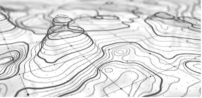
Figure 4: Graphical visualization of how the surrounding topographical information could be represented, as discretized altitude changes. In this work the topography will be represented as a slope angle for each discretized spatial point. [22]

5.1.6 Pulse and Glide (PnG)

Pulse and glide is the name of the phenomenon of alternating between accelerating at optimal, high load operation points, often at a quite high torque, and freewheeling, i.e. engaging the neutral gear. This phenomenon is, rather naturally, occurring when allowing

(20)

freewheeling to be possible in an optimization-based controller. Since it have been proven that most HDVs have their fuel efficiency sweet spot at high operation points and that alternating with freewheeling, although engaging neutral gear injects a small amount of fuel into the engine in order to keep it running, is more fuel-efficient than coasting with a given gear. This due to the fact that the mean fuel consumption of freewheeling and an effective gear is lower than constantly using an optimal gear. This have been shown in the work by Ohlsén and Sten [15] and does also appear in the simulation results of Mancino [17]. It also occurs in the work by Turri [9] when enabling freewheeling in the non-cooperative platooning proposal.

Apart from the fuel aspects of PnG, one ought also to consider other aspects such as rider comfort. This technique would imply that the engine would work at a rhythmical oscillating behaviour rather than at a dull continuous soundscape. Since truck drivers spend a lot of time in the cockpit this might be a problem to consider. But, since this thesis is of technical points of views rather than ergonomically, this will be disregarded in case of occurrence in the implementation.

5.1.7 Optimization solver

In the line of thought regarding optimal control explained in Section 5.1.1, one can generalise the optimization problem within the field of mathematics and computer science into the following; the optimization problem is the problem in finding the best solution in the set of all feasible solutions. The problem could be discrete, where one might look for an integer, or it could be continuous whereas one includes constraints in order to solve the problem. This thesis will formulate its problem with discrete variables such as gears and discretized continuous variables such as kinetic energy.

The optimization problem formulation will often be of a standard type where one wants to minimize an objective function, sometimes recalled as the cost function. In finance it could appear as the utility function, where the problem instead is to maximize. Regardless of the choice of notation, this function can be seen as the goal of the problem, hence the optimal solution will be heavily dependent on the choice of this formulation. For example, in the context of this thesis, since fuel-efficiency is one of the main targets, fuel consumption might be a good component in the cost function.

The methodology of choosing an appropriate optimization solver for the given optimiza-tion problem is a science itself9_{, so without digging too deep, only the method investigated}

in this thesis will be explained here. The used method is called dynamic programming (DP) and was developed by the mathematician Richard Bellman in 1954[18]. Here, DP will be used to solve the optimal control problem by dividing it into a collection of less complex optimal control problems and by exploiting the overlap of these sub-problems. It is said that the problem have optimal substructure if it can be solved opti-mally by breaking it down in this way and finding optimal solutions to the sub-problems. DP is also the chosen method in the implemented work by Turri [9] and by Alam et al. [11].

9_{Matlab, which is the programming environment used during most implementations of this work,}

have even made a toolbox function in order to aid the choice of optimization solver and an associated documentation for it in its latest update (2020a)

(21)

The complexity of the DP approach is O(NMT ), where N is the dimension of the states, M the dimension of the control signals and T the length of the time-horizon [9]. In comparison with a naive approach, one can conclude that DP is significantly more computationally efficient for large T . It also provides an intrinsic feedback law through its recursive formulation. Note, however, that the complexity is linear in the amount of possible states N but that this number grows exponentially with the dimension of the states when discretizing the continuous variables. This is commonly known as Bellman’s "Curse of dimensionality" [19]. This result in the soft constraint that for a DP formulation, one needs as few states as possible in order to keep the computational complexity feasible for real-time implementations.

5.2 Platooning control

The first appearance of automated platooning control using short inter-vehicular distances is shown by General Motors in a promotional film made in 1939, predicting modern life in 1960, named To New Horizons [20]. In the film, it is predicted that short inter-vehicular distances are maintained using automated radio control and physical latitudinal aid in forms of curved road sides are to be implemented. Similar visions are projected into the present but with newer approaches. Current state of the art platoon control strategies for HDVs might still be in the research stage but are expected to be deployed in the upcoming years [13]. The following two subsections will describe two clear distinctions of platooning strategies which will be of major importance when synthesizing a proposed architecture.

5.2.1 Cooperative platooning

A cooperative structure means that inter-vehicular communication in some way is en-abled. The cooperative concept is not necessarily bounded by certain communication protocols or by which signals that are shared, rather the fact that it is enabled. It has been proven that such a cooperative strategy would be significantly effective with regard to fuel-consumption but might become unfeasible due to the computational complexity.

Alam et al. [21] proposes a distributed linear-quadratic-Gaussian (LQG) control strat-egy which collects each individual vehicle’s fuel-optimal speed trajectory and selects the one that is most feasible to be the speed trajectory for the whole platoon. Turri [9] pro-poses a centralized cooperative control architecture using a platoon coordinator above each vehicle controller and a fleet layer which is above the platoon coordinator. The platoon coordinator communicates the optimal speed trajectory to individual vehicle controllers such that fuel consumption for the whole platoon is minimized, are feasible for all membering vehicles and satisfies the average speed condition required by a fleet layer at the same time.

5.2.2 Non-cooperative platooning

A non-cooperative structure would be a control system independent of inter-vehicular communication. Each vehicle would minimize its own fuel-consumption, with possible regard to concepts such as topography information or adaptive collision control. This

(22)

would result in sub-optimal performance for the platoon as a whole since there is unfea-sible to incorporate such a reference without communication enabled.

Turri [9] investigates a non-cooperative approach using a combination of some of the above mentioned concepts such as LAC, ACC, PnG and DP. The simulations shows fuel-saving potential of up to 18% compared to the lead vehicle, which uses LAC without freewheeling (PnG). Although non-cooperative does not posses the same potential as the cooperative approach, the shown reduction in fuel consumption is arguably significant. Note, however, that only two vehicles were investigated where solely the following vehicle had freewheeling enabled.

5.3 Modeling

There are different ways of describing a system and through a model, often derived from physical observations or measurements like forces and torques, is a commonness. In this subsection a brief exploration of how different recent studies in the area of fuel-efficiency optimal platooning are modeling their system. The description of the model that this thesis proposes can be seen in Section 6.

5.3.1 Longitudinal vehicle dynamics

Since most platooning solutions only handles longitudinal vehicle control it does make sense to describe the vehicle by its longitudinal dynamics acting on the system. Using Newton’s second law, Turri [9] and Ohlsén and Sten [15] expresses the dynamics in terms of traction, braking and gravitational forces, drag and rolling resistances. Mancino [17] uses a similar model description but without braking forces. Hovgard and Jonsson [16] are expressing some dynamics in terms of power, which becomes analogous since power is defined as force per distance over time or, P = dW

dt where P denotes power, t denotes

time, d

dt denotes derivative over time and W denotes work which is defined as W = F x

where F denotes force applied on the distance x.

Each one of these actuators are then modelled on an individual level. It could be from a known physical relationship, then often with a closed-form expression or it could be a data-driven model, for example, trained as a regression given data measurement points. In the coming subsections some models connecting these actuators with constraints or the cost function will be presented. The constraints and the cost function stems from features of the nature of the problem, hence might have room for some differences depending on the approach of the solution.

5.3.2 Drivetrain model

The drivetrain consists of all components of the powertrain, i.e. the components that converts fuel to movement, except for the engine. Turri [9], Ohlsén and Sten [15] and Hovgard and Jonsson [16] clearly states the assumption that the engine inertia is negligible with respect to the mass of the vehicle and disregards it from the drivetrain model, hence the drive shaft is assumed to be stiff. Mancino [17] adds a mass factor that takes in consideration the rotation of components inside the vehicle when expressing the engine force.

(23)

5.3.3 Engine model

The model of the engine relates how the amount of injected fuel corresponds to the output of the engine, often denoted in Nm as torque. Ohlsén and Sten [15] presents three engine models of different levels of complexity and sophistication. Namely Willans Line Approximation, Extended Willans Line Approximation and Complete Mean Value Engine Model with increasing complexity respectively, whereas the Extended Willans Line Approximation were implemented in the final simulation.

Both Mancino [17] and Turri [9] uses an fuel-efficiency map as model, more specifically the latter work uses the brake specific fuel consumption (BSFC). An efficiency map in this context can be seen as a function, (R × R) → R, which, for each pair of torque and RPM, maps the corresponding fuel consumption for that specific engine. Given this map one would then want to optimize in order to find an, at least, local optimum. A graphical parable of optimizing such a map is to find the highest mountain in a certain area such as in a country. The borders of the region would represent the constraints of the map, the geographical longitudinal and latitudinal directions would represent the engine speed and torque and lastly the altitude of the ground would represent the fuel-efficiency or the BSFC.

5.3.4 Transmission

Gear shifting, sometimes denoted as the transmission, inside a vehicle fundamentally works at delivering a spectrum of rotational speeds for the wheels given a torque value due to the different gear ratios. The reason for using transmission is that an ICE, in most use cases, needs to work at high operating speeds, whereas those speeds are usually not suited for, e.g. starting and stopping.

Ohlsén and Sten [15] uses a gear shifting model that reduces the produced net engine torque to zero, engages neutral gear, synchronizes the engine speed to the required speed from the new gear, engages this new gear then increases the net engine torque. This model is a simplified version of the one presented by Petterson and Nielsen [24] and works quite well with the assumptions that the driveline is stiff.

Turri [9] proposes, for cooperative platooning, a gear manager control layer between the individual vehicle controllers and the platoon coordinator, which optimizes gear se-lection and the gear shift timing. The optimization aims at minimizing fuel-consumption and deviations from speed and inter-vehicular distance references.

As mentioned in Subsection 5.1.6, when allowing freewheeling, i.e. neutral gear into the gearbox model, the optimization might result in an alternating behaviour, known as PnG. Ohlsén and Sten [15] focuses their simulations, consisting of two vehicles, at PnG by allowing freewheeling on both vehicles and each one separately. Turri [9] also focuses on this in some of the simulation cases for non-cooperative platooning, where also two vehicles were investigated, but only with the following vehicle allowing freewheeling.

(24)

5.3.5 Platoon model

Since the benefits from platooning stems from the fact that short inter-vehicular distances reduces air drag, this needs to be modelled in some way, in order to capture its behaviour. Alam [12] and Ohlsén and Sten [15] uses a longitudinal model for scaling the air drag coefficient, depending on the length of the inter-vehicular distance and the position in the platoon. Here, the models are determined through empirical measurements. Ohlsén and Sten uses a relation which scales the air drag coefficient non-linearly but adapts the linearization presented by Kemppainen [25].

(25)

6 Modeling

Through a model, a system can be represented. In technical contexts such as this, it can be regarded as a mathematical model, whereas the system gets described using mathematical concepts and notations. Here the models proposed will describe how different parameters or states such as velocity depends on other parameters such as aerodynamic resistance. These dependencies could be known or unknown, where in the latter case one might use another model to describe the relationship.

6.1 Thesis restrictions

In this thesis, the complete models used for describing the dynamics of the vehicle, the surrounding and the interaction between vehicles are obtained from Scania. The set of models are at such a complex level that it expands way past the scope of this thesis, to derive and define each detail. The purpose of the thesis is to investigate and design the control architecture needed for enabling platooning for heavy-duty hybrid vehicles, not to model its parameters. Hence, the models contained in the control unit will be described as they are relatively simplified but does not compromise the relationships in which they are describing at a too large extent.

6.2 Longitudinal dynamics

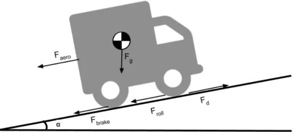
Since we are solely investigating a longitudinal control, we can look at the forces acting on the HDV, when it moves in one dimension to formulate an appropriate model. The forces acting on the vehicle in motion can be seen in Figure 5. Here we see one propulsive drive force Fd, stemming from the engine, which drives the vehicle forward. The rest of

the forces described in the Figure are denoted resistive forces, since they are acting in the opposite direction of the drive force.

(26)

Figure 5: Graphical illustration of the forces acting on the vehicle when considering longitudinal dynamics.

Using Newton’s second law of motion, ΣF = ma, one can derive the longitudinal model as following

Fd− Faero− Froll− Fbrake− Fg = m

dv

dt = f (x, u, s) (6.2)

where Fd denotes the drive force, Faero denotes the aerodynamic resistive force, Froll

de-notes the rolling resistance, Fbrake denotes the braking forces, Fg denotes the longitudinal

component of the gravitational force, m denotes mass, dv

dt denotes the derivative of the

velocity with respect to time, or with other words, acceleration. x = [E g tg]0 denotes the

states which are kinetic energy, current gear and time-gap to the preceding vehicle respec-tively. u = [Mnet g]0 denotes the control signals net torque and current gear respectively.

s denotes the position of the vehicle, which will be connected with the slope. 6.2.1 Drive forces

The driving force is the force which moves the vehicle forward and is noted as Fd in

Figure 5. The drive force is defined as the force acting on the final drive axle where the wheel sits. The parts and components from the net torque out of the engine to this final drive are called the drive line. The drive line is assumed to have no torison, i.e. to be modelled as stiff, and the clutch is assumed to have no slip.

Given the current engine speed, one can calculate the net torque coming out of the engine. The torque out of the transmission is determined by the net torque multiplied by the gear ratio of the transmission.

(27)

where gtis the ratio of the transmission and Mnetdenotes the net torque from the engine.

Mt will now be transferred from the so called propeller shaft onto the drive shaft where

the wheels sit. This transformation is done by fixed gear ratios in the final drive.

Mf inal = gf inalMt (6.4)

where gf inal denotes the fixed gear ratio of the final drive and Mf inal denotes the final

torque that will be giving the propulsive drive force to the vehicle. Fd=

Mf inal

rw

(6.5) Hence, equation 6.3 to equation 6.5 gives the following drive force relation.

Fd= Mnet

gtot

rw

(6.6) where gtot denotes the total gear ratio from the propeller shaft to the final drive shaft.

6.2.2 Resistive forces

The resistive forces are formulated as three different forces, acting naturally against the direction of the drive force, namely the rolling resistance Froll, the aerodynamic resistance

Faero, the gravitational force Fg. There are also two forces acting against the propulsion

of the vehicle which is the braking force Fbrake and the relative slip of the wheels against

the surface denoted ωwheel. Parameters can be found in Table 3.

Notation Value Unit

m 40e3 [kg] rw 0.506 [m] Cd 0.6 [1] Cb 0.58e-2 [1] CaF 5.64e-5 [1] CrrisoF 5.36 [1] A 10 [m2] g 9.81 [N/kg] vISO 80 [km/h] ρair 1.29 [kg/m3]

Table 3: Table of parameters used for modelling resistive forces.

The rolling resistance occurs when a body, here the tire, rolls over a surface, here the road. The amplitude of the rolling resistance depends on the material of both the surface and the body and the tire contact patch. Loosely speaking, a smaller contact area between the tire and the road results in a lower rolling resistance, given equal materials.

(28)

The model used for describing the rolling resistance is referred to as The Michelin rolling resistance model and consists of a second order polynomial in vehicle velocity:

Froll(v) =

((v2_{− v}2

iso)CaF + (v − vISO)Cb+ CrrisoF)mvg cos(α)

1000p1 + rw

2.7

(6.7) where v denotes the velocity of the vehicle in km/h, mv denotes the mass of the vehicle,

g denotes the gravitational constant, α denotes the slope of the road in radians and rw

denotes the radius of the wheel. viso, CaF, Cb, CrrisoF denotes constant parameters shown

in Tabular 3.

The aerodynamic resistance could be denoted as the friction force between a moving object and the air surrounding it. The force both consists of the form drag, given by the geometrical shape of the object and the skin fiction, given by the materialistic properties of the object. This force is formulated from the, rather classical, quadratic model:

Faero(v) =

ρairCdAv2

2 (6.8)

where v denotes the velocity of the vehicle in m/s, ρair denotes the density of the air,

Cd denotes the aerodynamic resistance coefficient and A denotes the frontal area of the

vehicle. Each constant parameter are shown in Table 3.

As a remainder, the aerodynamic resistance force is the force which platooning aims at reducing, both due to the decreased aerodynamic pressure against the frontal area and due to the decrease in backwards-pulling turbulence forces. Since the aerodynamic resistance coefficient Cddepends on the preceding and following vehicles, instead of having

it constant, it will be denoted by the following non-linear model: Cd(d) = cd(1 −

fi(d)

100 ) (6.9)

which scales the aerodynamic resistive coefficient cd. fi denotes the non-linear function,

dependent on the distance to the preceding vehicle d.

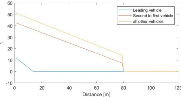
This thesis have applied a linearization made by Kemppainen [25]. The linearization can be seen in Figure 6 and is stated as following

f1(d) = (-0.9379d + 12.8966, if 0 ≤ d ≤ 15 0, otherwise (6.10a) f2(d) = (-0.4502d + 43.0046, if 0 ≤ d ≤ 80 0, otherwise (6.10b) f3(d) = (-0.4735d + 51.5027, if 0 ≤ d ≤ 80 0, otherwise (6.10c) fi(d) = f3(d), i ≤ 4 (6.10d)

where d denotes the distance between the vehicle and the preceding vehicle, except for the leading vehicle where the distance is relative to the following vehicle. The function index i denotes which vehicle the model serves, where 1 denotes the leading vehicle.

(29)

Figure 6: Illustration of the linearization by Kemppainen.

The gravitational force works as a resistant force in uphill situations while on downhill sections it will help the vehicle in its direction and will affect the vehicle, in its longitudinal directions, minimally when the road slope is close to flat. Since the gravitational force acts in the direction of the center of the earth, its resistive component will be fraction of the whole gravitational force acting on the vehicle, given by the trigonometric relationships, resulting in the following model:

Fg(α) = mg sin(α) (6.11)

where m denotes the mass of the vehicle, g the gravitational constant and α the road slope in radians.

Depending on the tire material and the surface of the road, the wheels might slip during parts of the drive. To measure the relative slip of the wheels relative to the road, the following model is used;

ωwheel(v) =

v(1 + αFt)

rw

(6.12) where v denotes the velocity of the vehicle in m

s, α denotes the slip coefficient and Ft

denotes the total propulsive force delivered by the wheels.

6.3 Optimization problem statement

The optimization problem of fuel-efficient planning can be formulated as a minimization problem, where one wants to minimize the fuel consumption mf, which will be our cost

(30)

regard to the control signals and the state variables.

minimize mf (6.13a)

subject to T ≤ To (6.13b)

feasible vehicle dynamics (6.13c)

In this thesis, the time constraint will be incorporated in the time-gap state, which is relative to the vehicle in front as the time it takes for the vehicle to reach the leading position. The leading vehicle will have its time-gap relative to a fictive vehicle. This fictive vehicle is driving with a constant given speed. The maximum and minimum lim-its of the time-gap of the leader will then act as a window, in which the leader can be positioned, to yield a mean speed close to the set speed of the fictive vehicle. In this manner, one incorporates the time constraint without having to either set a constant limit nor fine-tune the β parameter of the relaxed version. The fine-tuning would be an extensive and computational burden on the optimization solver since it would be needed to be tuned in every time-step.

The feasible vehicle dynamics includes the models and constraints for the drive forces, resistive forces and transmission.

minimize mf (6.14a) subject to T ≤ To, (6.14b) mdv dt = f (x, u), (6.14c) Emin ≤ E ≤ Emax, (6.14d) g ∈ {g0, g1, ..., gmax}, (6.14e) tg,min ≤ tg ≤ tg,max, (6.14f) Mmin ≤ M ≤ Mmax, (6.14g) where x = {E g t}0, (6.14h) u = {M g}0 (6.14i)

6.4 Micro-transactions

6.4.1 Problem statement

There are some inherent problems with centralized platooning that works as a resistant force against implementing such a system in reality. One problem being the contradiction between two major strategies for driving as fuel-efficient as possible. When minimizing fuel-consumption, driving at short inter-vehicular distances becomes a key to reduce the air drag of the platoon. A smaller inter-vehicular gap implies a greater air drag reduction, which would limit the flexibility to vary speed e.g. in hilly terrains. Thus, the trade-off between speed flexibility and inter-vehicular distances, with regard to fuel-efficiency, will have to be considered.

(31)

man-ufacturers and freight transportation companies. Since vehicles closer to the front, espe-cially the leading vehicle, will experience less of the fuel-saving aspects as the rear part of the platoon, no vehicle would want to be in the front. Hence, without individual in-centives members of the platoon would not want to change their speed profiles according to other members, even though the whole platoon would save more fuel as a group. If one is to implement a platoon coordinator in practice there will be a channel of com-munication between vehicles, most likely, containing some sensitive information. This information could be with regard to masses, resistances and engine efficiencies and would not be shared between competitive brands without some kind of protocol, acting as a safety net. Without a safety net, the system could easily be exploited, for example by sending false values in order to achieve larger benefits from the profit of the whole pla-toon. In the same line of thought, regarding communication, one would have to address the problem of trust when implementing a platoon coordinator. Every member of the fleet needs to be ensured that the platoon coordinator is not giving any brand, vehicle or freight operator special advantages or disadvantages.

6.4.2 Solution10

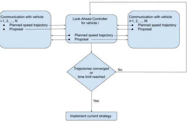
The proposed solution to the above mentioned problems of the centralized platoon co-ordinator is to let each vehicle plan its fuel-optimal driving strategy with knowledge of all surrounding fuel-optimal strategies from the rest of the platoon. When contradictions occur, between fuel savings by short inter-vehicular distances and speed variations, the problem is solved through automatic negotiations and micro-transactions between the platooning members.

All participating vehicles in the platoon are equipped with an LAC, which plans the speed trajectory for that vehicle for a given time-horizon. If only implemented in one vehicle, that vehicle would then execute that planned speed trajectory as the current strategy. In the case of multiple vehicles, which most of the time will be the case, the current strategy will be obtained through an iterative process. All vehicles initial planned speed trajectory will be communicated to the rest of the platoon thenceforth an updated speed trajectory will be calculated in order to close the iterative loop. A schematic representation of the mentioned control scheme is presented in Figure 7.

If the LAC notices that any vehicle’s speed trajectory interferes with its creation of its own fuel-efficient trajectory, it will pose a proposal to that obstructing vehicle. If, for example, the LAC notices that it will have to apply brakes in the upcoming downhill, in order to avoid a collision, it will calculate the amount of fuel that the brake application will cost. This brake cost will then correspond to an economic value, say a price. If the preceding vehicle is prepared to move faster, such that the following vehicle does not have to apply braking, at a compensation smaller than the calculated cost of braking but larger than the cost of applying that acceleration, both parties will gain from this 10_{The proposed solution is, during the writing and presenting of this thesis, which will occur June}

25th and June 26th 2020, under pending patent application as the invention 2020-0092 "System for cooperative platooning using micro transactions" under Scania CV AB and the names of my supervisors and me, Henrik Svärd, Svante Johansson and Philip Ahl, respectively.

(32)

agreement hence the proposal gets accepted.

Figure 7: A schematic description of the control scheme to the proposed solution, N denotes the number of vehicles in front of vehicle i and M denotes the number of vehicles behind vehicle i.

The planned speed trajectories of each vehicle member will be updated repeatedly, with new information and proposals from surrounding vehicles after each iteration, until convergence of all speed profiles, i.e. there are no new proposals appearing that are profitable for any members of the platoon. This situation corresponds to what, in terms of game theory, is defined as a Nash equilibrium. Informally citing the definition, a strategy profile is a Nash equilibrium if no one can do better by unilaterally changing his or her strategy. In this case, this would occur when the cost of changing a speed trajectory is greater than the cost of change to another vehicle, which leads to the fact that the platoon strategy has reached an, at least, local optimum. Practically speaking, since the LAC may consist of an optimization algorithm, the implementation will be readily incorporated in the cost function.

(33)

7 Control strategies

This Chapter takes the reader through the chosen control strategies and is set up as follows. Section 7.1 explains the details of implementing the LAC, from the discretization to the optimization solver. This is followed by Section 7.1.4 which shows the verification of the LAC system. Similarily Section 7.2 shows the implementation of the proposed MTC followed by Section 7.2.1 which verifies it.

7.1 LAC implementation

All vehicles are equipped with an LAC control system, making each and everyone capable of finding its optimal path given the future terrain, such as visualized in Figure 8. The mentioned micro-transaction system will be built upon this, using its core optimization as baseline. Therefore it is of considerable importance to verify the LAC before implementing the micro-transaction system in order to save time and to ensure its performance. The following subsections will describe the optimization process within the DP framework and how to extend it towards a micro-transaction-based system.

Figure 8: Visualiation of the LAC system data flow. 7.1.1 Discretization

In order for the DP algorithm to be able to work with the optimal control problem, men-tionned in 6.3, discretization is needed. Both control signals and states are discretized.

(34)

Since the choice of gearing is discrete by nature, as integers, it does not need to be changed. The control signal for torque is discretized into A evenly spaced intervals and the states energy and time-gap will be discretized into B and C respectively. The future-planning of the DP algorithm, the horizon, will be done over a spatial discretization of D evenly spaced points. With this discretization one get the problem 6.14 can be rewritten as minimize mf(x, u) (7.15a) subject to t ≤ to, (7.15b) mdv dt = f (x, u), (7.15c) E = mv 2 2 , (7.15d) Ei ∈ {Ei1, E 2 i, ..., E D i }for i = 1, 2, ..., B (7.15e) gi ∈ {gj1, g 2 i, ..., g D i } for i = 1, 2, ..., gmax (7.15f) tg,i ∈ {t1g,i, t 2 g,i, ..., t D g,i} for i = 1, 2, ..., C (7.15g) Mi ∈ {Mi1, Mi2, ..., MiD} for i = 1, 2, ..., A (7.15h) where x = {E g t}0, (7.15i) u = {M g}0 (7.15j)

7.1.2 Dynamic Programming (DP) Algorithm

The DP algorithm solves the optimal control problem which will be spanned up by both discrete integers and real variables discretized as described earlier. An illustration of the state discretization can be seen in Figure 9. This tensor may expand beyond the scope of the visual representation and is solved for each time step until the end of the horizon in the DP algorithm.

for all x ∈ XN (7.16a)

let JN(x) = JN∗(x) (7.16b)

end for (7.16c)

for k = N − 1, N − 2, ..., 0 (7.16d)

for x ∈ Xk let (7.16e)

Jk(x) = min u∈Uk

{ξk(x, u) + ˜Jk+1(fk(x, u))} (7.16f)

end for (7.16g)

end for (7.16h)

(35)

The pseudo-code of the DP algorithm is shown in Equation 7.16 where ˜J denotes the interpolated cost-to-go, ξ denotes the discrete step-cost, x denotes the states, u denotes the control signals and fk(x, u) denotes the discretized model.

Figure 9: Visual representation of the discretization. Here, gear is integer valued whilst energy and time-gap is real valued.

7.1.3 Cost-to-go

In order to evaluate the cost of moving the vehicle from one position with its corresponding states, to a new position, one needs to calculate the cost-to-go. Since we do not have position as a state, all applicable states will be considered given the boundaries. One can view it as finding the optimal pair of energy, i.e. velocity, and gear, given that the time-gap is not exceeding its limits with some elbow room. In each time step of the optimization the kinetic energy is calculated from Equation 6.2 and updated as follows.

Enew = Eold+

2∆s(Fd− Faero− Froll− Fg− Fbrake)

m (7.17)

where ∆s denotes the step length in the spatial discretization. The velocity is calculated by the square root operator of the kinetic energy which is a computational costly operator, but at which this work is not mainly aiming at optimizing. The time-gap is updated using the time it takes the vehicle to drive one segment length, δs and is updated in the following manner. tg,new= tg,old+ ∆s 2 ( 1 vnew + 1 vold ) (7.18)

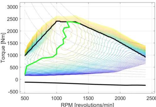
The new energy state is used to calculate the rpm of the engine, which in combination with the control signal torque is used to with an efficiency map of the engine. The efficiency map is used as a look-up-table with constant values given a pair of torque and rpm and is visualized in Figure 10. Let us call the discrete cost gained from this efficiency map ξ(u, x).

(36)

Figure 10: Visual representation of the specific fuel consumption of the engine given a pair of torque and rpm, given in g/kWh. Black, thick lines denotes the limits, the green line denotes the path of the fuel optimal pairs and the coloured contour lines provides a representation of the fuel efficiency where light yellow denotes a low fuel consumption thus high efficiency, whilst purple and profound blue denotes high fuel consumption thus low efficiency.

Using the models through the efficiency map we can now calculate the cost of going from one discrete state to another one. Quite often, the optimization problem will not only manoeuvre discrete points, so to yield the full cost-to-go to a state which might be in between two discrete states, we will need to add an interpolating cost in-between two energies or two time-gaps.

For a given energy, Enext, linear interpolation between the costs J(En, g, tg, m) and

J (En+1, g, tg, m)where En < Enext < En+1and the interpolated value is denoted as ˜J (u).

The full cost-to-go is yielded as the sum of the interpolating cost and the discrete cost as follows: JtoGo= min u∈U,x∈X ˜ J (u, x) + ξ(u, x) (7.19) 7.1.4 Verification of LAC

In order to ensure that one can believe that the LAC is functioning properly, different verifications were made. The verifications are simulated on fully designed situations, where one can test a given hypothesis. The first case is to test the LAC on a flat road. Here the hypothesis states that, given the initial states, the vehicle should accelerate or de-accelerate into its optimal operation points until the horizon ends. Here, the horizon length is 4 km. In this context, optimal operation points means the pair of torque and revolutions per minute that the engine consumes the least amount of fuel, hence the most fuel-efficient situations of the engine. In this simulation a conical penalization is applied on the end states time-gap and energy, favouring certain states for the vehicle to end at.

(37)

Meaning that it will tend to end its planned trajectory at the same spot each run, for both vehicles to be comparable in terms of fuel consumption. The time-gap penalty is quadratic and centered around the initial time-gap, so it is assumed that the vehicles will make efforts for ending at similar states.

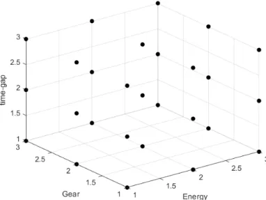
Since no slope is introduced in this verification case, a following vehicle would, if working properly, find a sweet-spot distance behind its leader in order to maximize its aerodynamic benefits. In Figure 11 and 13 one can see the efficiency map and simulated operation points for the leader and follower, vehicle 1 and 2, respectively. The black borders defines the feasible upper and lower limits of the torque and rpm pairs. The green route shows the optimal, in terms of fuel-efficiency, path for different levels of torque. The blue dots determine at which operation points the simulation have chosen and for how long, determined by the size of the dots where larger dots implicate longer time.

Figure 11: The efficiency map of the flat surface LAC verification case for the leading vehicle.

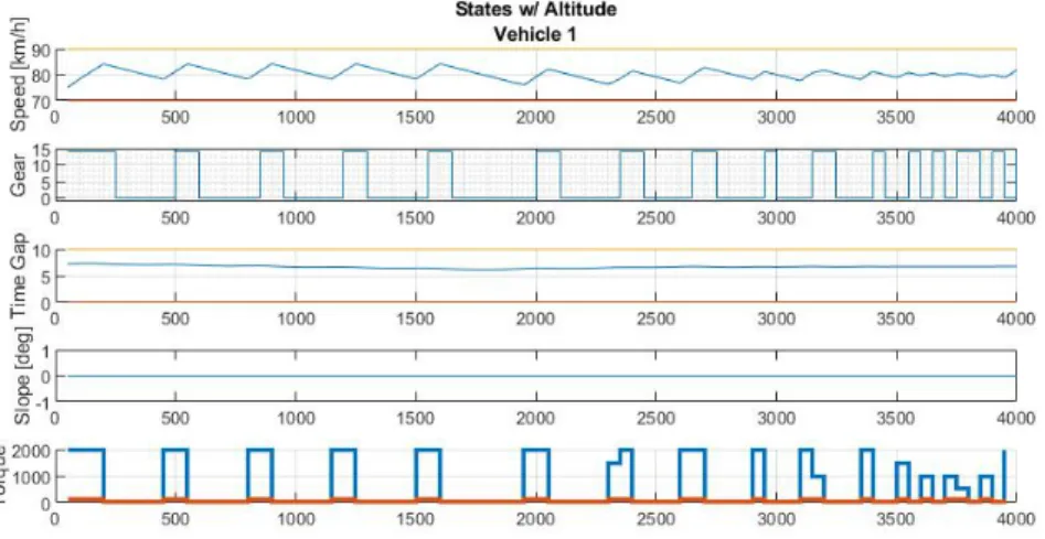
Figure 12: The state evaluation of the flat surface LAC verification case for the leading vehicle.

(38)

In the most upper graph in Figure 12 one can see that the vehicle quite directly initiates PnG, alternating between high load operating points at optimal torques and freewheeling. The PnG frequency for the leading vehicle, i.e. the rate of change between alternations, is around 0.5 km and can be seen in Figure 12 and for the follower around 1 km which can be seen in Figure 14. It is reasonable that both vehicles share the same PnG frequency or an multiple of each other since it yields a close to constant time-gap. If the time-gap between the vehicles would vary and oscillate, one can argue that an aerodynamic sweet spot would not be found, or at least hard to find, which would not be optimal for either vehicle. Here, the follower close to the same frequency as the leader, with parts of or that the whole pulse have lower magnitude. This is reasonable since it ought to gain some aerodynamic benefits from slipstreaming, since it pulses the same time as the leader, it ought to accelerate less each time. The following vehicle have a average speed of 100.01% of the leader’s average speed but a fuel consumption at 82.07% relative to the leader, saving 1.03 kr compared to driving alone, which probates the hypothesis as well. Since the average speed of the follower is penalized when deviating from the average speed of its leader, it is reasonable that this percentage is close to 100%. One can also notice that small adjusting acceleration pulses are applied in the very end for the vehicle to land at the desired states.

Note that the drive cost shown in Figure 11 and 13 is calculated relative to the initial speed and outgoing speed, such that the price of the end state is incorporated. Also a fixed diesel price at 10 kr/l is used among all prices in this work, in order for the price to be as comprehensible and intuitive as possible. In both LAC verification cases, both vehicles masses are set to the same at 30 tonnes and are driving at 75 km/h at a distance of 50 m from each other.

Figure 13: The efficiency map of the flat surface LAC verification case for the following vehicle.

(39)

Figure 14: The state evaluation of the flat surface LAC verification case for the following vehicle.

In the second verification case of the LAC, a hill is introduced. The hill is designed such that it have a constant change of slope. The angle starts at 0.5 degrees and ends at negative 0.5 degrees on the whole 4000 meter horizon. The vehicles are here expected to accelerate towards the crest of the hill, in order to release at least some of its acceleration before the crest, in such a way that it will have to brake none or minimally during the downhill. The following vehicle should have a similar behaviour but with an earlier release of the acceleration since it should be able to benefit from the air drag reduction.