Analysis of heat recovery in supermarket
refrigeration using carbon dioxide as refrigerant
Amir Abdi
Master of Science Thesis
KTH School of Industrial Engineering and Management Energy Technology EGI-2014-017MSC
Division of Applied Thermodynamics and Refrigeration SE-100 44 STOCKHOLM
Master of Science ThesisEGI 2014:017MSC Analysis of heat recovery in supermarket refrigeration
system using carbon dioxide as refrigerant
Amir Abdi
Approved Examiner
Samer Sawalha
Supervisor
Samer Sawalha
Commissioner Contact person
Abstract
The aim of this study is to investigate the heat recovery potential in supermarket refrigeration systems using CO2 as refrigerants. The theoretical control strategy to recover heating demand from refrigeration
system is explained thoroughly and the heat recovery process from two existing supermarket using CO2
booster units is analyzed and evaluated. The measured data of refrigeration systems is obtained through Iwmac interface, processed using Excel and Refprop. The aim is to see what control strategy is used in these systems and weather it matches the theoretical one and at what level heat is recovered from the system.
Besides, a simulation model is made by EES to investigate the potential of higher rate of heat recovery in the supermarkets. The simulation results are compared with field measurement and validated by measured values. Then, the ability of refrigeration system to do heat recovery at quite high rates for covering the total heating demand without using parallel heating system is evaluated and efficiency of the system is calculated. At the next step the heat recovery potential at other refrigeration solutions such as R404A conventional and CO2-ammonia cascade systems are studied and the results are compared to booster
units. Finally, the potential for selling heat from the refrigeration system in supermarket to district heating network is investigated. Two different scenarios are made for such purpose and the results are evaluated. The heat recovery control strategy of existing supermarkets does not match the theoretical strategy and regarding the capacity of the system, heat is recovered to low extent. Simulation shows that heat can be recovered to higher extent at quite high heating COP of 3-5. Additionally the other heat recovery solutions for R404A conventional and CO2-ammonia cascade systems are found to be competitive to CO2
booster system. The analysis of selling heat to district heating network shows that CO2 booster system is
capable of covering the demand at reasonable heating COP as the first priority and selling the rest to district heating network at heating COP of 2 as second priority.
Acknowledgements
I would like to express my deep gratitude to my supervisor, Samer Sawalha, who supervised my work and helped me to do it. Additionally I am thankful to Mazyar Karampour who assisted my friendly to finish this work. Finally I would like to thank my family who supported me greatly during my whole life and during my study at KTH as well.
Content
Abstract ... 2 Acknowledgements ... 3 Content ... 4 List of Figures... 7 Nomenclature...10 1 INTRODUCTION ...12 1.1 Background ...121.2 Aims and objectives...12
1.3 Methodology ...12
1.4 Limitations ...13
2 SUPERMARKET REFRIGERATION & HEAT ECOVERY SOLUTIONS ...14
2.1 CO2 as refrigerant...14
2.2 CO2 Properties ...14
2.3 Supermarket system solutions ...15
2.3.1 Indirect system ...15
2.3.2 Cascade system ...16
2.3.3 Trans-critical system...16
2.4 Energy usage in supermarket ...18
2.5 Heat recovery solutions...18
2.5.1 Heat pump connected to refrigeration system ...19
2.5.2 HVAC system connected to refrigeration system ...19
2.6 CO2 heat recovery analysis ...20
2.6.1 Optimum discharge pressure ...21
2.7 Heat recovery control strategy ...23
2.8 COP definition ...24
3 MASS FLOW RATE CALCULATION ANLYSIS ...26
3.1 Mass Flow estimation method ...26
3.1.1 Volumetric method ...26
3.1.2 Total efficiency method ...26
3.1.3 Heat balance method...27
3.2 Experimental analysis...27
3.2.1 Test rig description ...27
3.2.2 Methodology ...28
3.2.3 Results & Discussion...28
4 FIELD MEASUREMENT ANALYSIS...30
4.1 Description of supermarkets refrigeration system...30
4.1.1 TR2...30
4.1.2 TR3...32
4.1.3 Data retrieval...33
4.2 COP calculation analysis ...33
4.3 Control strategies for supermarket refrigeration systems ...34
4.3.1 Yearly analysis ...35
4.3.2 Monthly analysis ...37
4.3.3 Daily analysis...44
4.4 Analysis of heat recovery potential ...49
5 SIMULATION ANALYSIS ...53
5.1 Model description...53
5.2 Simulation results for different modes ...54
5.2.1 TR2...54
5.2.2 TR3...58
5.3 Monthly analysis...63
5.3.1 TR2...63
5.3.2 TR3...65
5.4 Sub-cooling effect for TR2 ...67
5.5 Analysis of heat recovery improvement in TR3 ...69
6 COMPARISON OF HEAT RECOVERY IN DIFFERENT SYSTEM SOLUTIONS...73
6.1 Simple comparison analysis ...73
6.2 Various system descriptions with alternative solution of heat recovery...76
6.2.1 CO2 -Booster...76
6.2.2 Ammonia- CO2 Cascade ...77
6.2.3 R404A Conventional ...78
6.3 Heating COP modification ...80
6.4 Results & Discussion ...80
7 ANALYSIS OF HEAT SALE FROM CO2 BOOSTER SYSTEM ...81
7.1 Heat sale to district heating...81
7.2 1st Scenario ...82
7.3 2nd Scenario ...83
7.4 Results &discussion ...83
8 CONCLUSION ...88
Bibliography ...89
List of Figures
Figure 1 - Thermal characteristics of CO2 VS Condensing temperature (Sawalha, 2008) ...15
Figure 2 - Indirect solution in supermarket refrigeration ...16
Figure 3 – Ammonia- CO2 cascade solution ...16
Figure 4 – CO2 centralized system solution ...17
Figure 5 –CO2 parallel system solution...17
Figure 6 – CO2 booster solution...18
Figure 7 - Heat recovery solutions connected to heat pump ...19
Figure 8 - Heat recovery solutions connected to heating system...20
Figure 9 - Parallel heating equipment connected in different ways to heating system ...20
Figure 10 - PH diagram of CO2 for different discharge pressure ...21
Figure 11 - Cooling COP VS discharge pressure for different gas cooler outlet temperature (Sawalha, 2008) ...22
Figure 12 – Cooling COP VS condensation temperature for different return temperature (Frelechox, 2009) ...22
Figure 13 - Controlled discharge pressure and gas cooler exit temperature VS heat recovery ratio (Sawalha, 2013) ...23
Figure 14 - Schematic layout of test rig at Energy technology department of KTH ...28
Figure 15 - Mass flow rate for direct measurement and different estimation methods...29
Figure 16 - Accuracy of different mass flow rate estimation methods ...29
Figure 17 - Schematic layout of TR2 supermarket ...30
Figure 18 - Schematic layout of refrigeration system at TR2 ...31
Figure 19 - Measurement layout of refrigeration system at TR2 ...31
Figure 20 - Measurement layout of water at TR2...32
Figure 21 - Schematic layout of refrigeration system at TR3 ...32
Figure 22 - Measurement layout of refrigeration system at TR3 ...33
Figure 23 - Measurement layout of water at TR3...33
Figure 24 - Monthly averaged measured values at TR2 - 2012...35
Figure 25 - Monthly averaged cooling demands and recovered heat at TR2 – 2012 ...36
Figure 26 - Monthly averaged measured values at TR3 - 2012...36
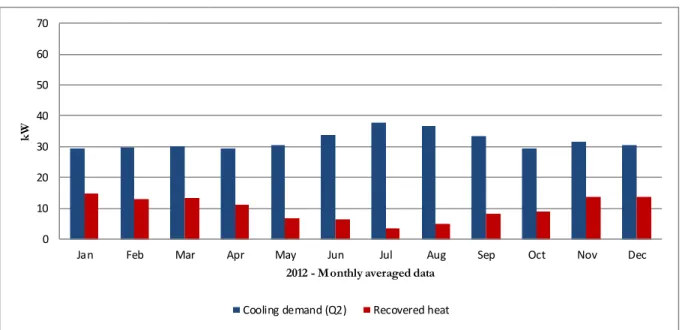
Figure 27 - Monthly averaged cooling demands and recovered heat at TR3 – 2012 ...37
Figure 28 - Measured values for October 2012 at TR2...38
Figure 29 - Measured values for November 2012 at TR2 ...38
Figure 30 - Measured values for December 2012 at TR2 ...39
Figure 31 - Measured values for March 2012 at TR2...40
Figure 32 - Measured values for April 2012 at TR2 ...40
Figure 33 – Measured values for October 2011 at TR3 ...41
Figure 34 - Measured values for November 2011 at TR3 ...42
Figure 35 - Measured values for December 2011 at TR3 ...42
Figure 36 - Measured values for January 2012 at TR3 ...43
Figure 37 - Measured values for November 2012 at TR3 ...43
Figure 38 - Measured values for December 2012 at TR3 ...44
Figure 39 - Hourly averaged measured values for December 17, 2012 at TR2...45
Figure 40 - Hourly averaged measured values for December 17, 2012 at TR2...45
Figure 41 - Hourly averaged cooling demands and recovered heat for December 17, 2012 at TR2 ...46
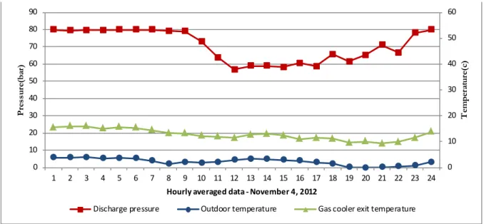
Figure 42 - Hourly averaged measured values for November 4, 2012 at TR3...46
Figure 43 - Hourly averaged measured values for November 4, 2012 at TR3...47 -7-
Figure 44 - Hourly averaged cooling demands and recovered heat for November 4, 2012 at TR3 ...47
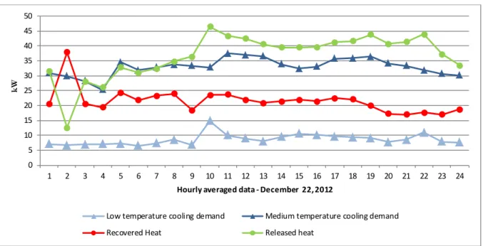
Figure 45 - Hourly averaged measured values for December 22, 2012 at TR3...48
Figure 46 - Hourly averaged actual values for December 22, 2012 at TR3 ...49
Figure 47 - Hourly averaged cooling demands and recovered heat for December 22, 2012 at TR3 ...49
Figure 48 - Monthly averaged cooling and heating demand for 2012 at unit KAFA1-TR2 ...50
Figure 49 - Monthly averaged cooling and heating demand for 2012 at unit KAFA2-TR2 ...50
Figure 50 - Monthly averaged cooling and heating demand for 2012 at unit KA3-TR2 ...51
Figure 51 - Monthly averaged cooling and heating demand for 2012 at unit KAFA1-TR3 ...51
Figure 52 - Monthly averaged cooling and heating demand for 2012 at unit KAFA2-TR3 ...52
Figure 53 - Schematic diagram of simulation model ...53
Figure 54 - PH diagram of simulated refrigeration cycle for different modes at TR2 ...55
Figure 55 - Heat load and measured discharge pressure during night time for some periods at TR2 ...56
Figure 56 - Heat load and measured discharge pressure during day time for some periods at TR2 ...56
Figure 57 - Comparison of calculated and measured values during day time for different periods at TR2.57 Figure 58 - Comparison of calculated and field measurement cooling COP during day time for different periods at TR2 ...57
Figure 59 - PH diagram of simulated refrigeration cycle for different modes at TR3 ...59
Figure 60 - Heat load and measured discharge pressure during night time for some periods at TR3 ...60
Figure 61 - Heat load and measured discharge pressure during day time for some periods at TR3 ...60
Figure 62 - Comparison of calculated and measured values during night time for different periods at TR3 ...61
Figure 63 - Comparison of calculated and field measurement cooling COP during night time for different periods at TR3 ...62
Figure 64 - Comparison of calculated and measured values during day time for different periods at TR3.62 Figure 65 - Comparison of calculated and field measurement cooling COP during night time for different periods at TR3 ...63
Figure 66 - Comparison of calculated and actual values during day time in December 2012 at TR2...64
Figure 67 - Cooling and heating COPs during day time in December 2012 at TR2...64
Figure 68 - Comparison of calculated and measured values during night time in December 2012 at TR3.65 Figure 69 - Cooling and heating COPs during night time in December 2012 at TR3 ...65
Figure 70 - Comparison of calculated and measured values during day time in December 2012 at TR3 ...66
Figure 71 - Cooling and heating COPs during night time in December 2012 at TR3 ...67
Figure 72 - Simulated values VS ambient temperature for borehole and gas cooler options ...68
Figure 73 - Comparison of COPs for borehole and gas cooler option ...68
Figure 74 Comparison of simulated and actual discharge pressure VS heat recovery ratio for return temperature of 35 ℃ ...69
Figure 75 Comparison of simulated and actual gas cooler exit VS heat recovery ratio for return temperature of 35 ℃ ...70
Figure 76 Comparison of simulated and actual cooling COP VS heat recovery ratio for return temperature of 35 ℃...70
Figure 77 Cooling COP VS gas cooler exit temperature for different return temperature ...71
Figure 78 Comparison of simulated and actual heating COP VS heat recovery ratiofor return temperature of 35 ℃...72
Figure 79 Schematic layout of simple refrigeration system with de-superheater used for heat recovery ....73
Figure 80 PH diagram for different condensation temperature for R404A ...74
Figure 81 PH diagram for different condensation temperature for Ammonia ...74
Figure 82 PH diagram for different condensation temperature for CO2 ...75
Figure 83 Heating capacity VS condensation temperature for three refrigerants...75 -8-
Figure 84 Heating COP VS condensation temperature for three refrigerants ...76
Figure 85 Schematic layout of heat recovery in cascade refrigeration system...78
Figure 86 Schematic layout of heat recovery in R404A conventional refrigeration system (Single loop) ...79
Figure 87 Schematic layout of heat recovery in R404A conventional refrigeration system (Separate loop)79 Figure 88 Comparison of heating COP for different solutions for return temperature of 30 ℃ ...80
Figure 89 Comparison of heating COP for different solutions for return temperature of 40 ℃ ...81
Figure 90 Schematic layout of heat recovery and refrigeration system 1st scenario ...82
Figure 91 Schematic layout of heat recovery and refrigeration system 2nd scenario ...83
Figure 92 Temperature profile of CO2 and water in 1st scenario ...84
Figure 93 Temperature profile of CO2 and water in 1st scenario ...85
Figure 94 Compressor work of different heat recovery solutions ...86
Figure 95 Heating capacity of different heat recovery solutions ...86
Figure 96 Cooling COP of different heat recovery solutions ...87
Figure 97 Heating COP of different heat recovery solutions ...87
Nomenclature
Abbreviations
HRR Heat recovery ratio
COP Coefficient of performance COSP Global coefficient of performance CO2 Carbon dioxide
FC Refrigeration operating on floating condensing mode HP Heat pump
HVAC Heating, ventilation, and air conditioning NH3 Ammonia
Symbols
E Electrical power [kW] h Enthalpy [kJ/kg.K] m Mass flow rate [kg/s] P Pressure [bar]
Q Heating or cooling capacity [kW] T Temperature [°C]
t Time [s]
V Volumetric flow rate Cp Specific heat [kJ/kg.K] α Thermal diffusivity [m2/s] 𝜌 Density [kg/m3] λ Thermal conductivity [W/m.K] η Compressor efficiency
Subscripts
bh Borehole br Brine DH District heating el Electrical f FreezingFC Refrigeration operating on floating condensing mode -10-
GC Gas cooler HR Heat recovery In Inlet is Isentropic LS Low stage
LT Low temperature, freezing level MS Medium stage
MT Medium temperature, chilling level Opt Optimal Out Outlet Tot Total v Volumetric 1 Condensation level/Heating 2 Evaporation level/Cooling -11-
1 INTRODUCTION
1.1 Background
Supermarkets are the commercial buildings with huge rate of energy consumption. The main demand which the refrigeration system is supposed to cover is cooling demand. But on the other hand, the building requires energy for heating purposes specifically in cold climates. Refrigeration system does reject high heating capacity to the ambient which could be used for covering the building heating demand. Recently, CO2 as natural refrigerant with low environmental impact is aimed to be used in new
installations. Additionally, special characteristics of CO2 around critical point and in trans-critical region,
enables the refrigeration system to recover considerable heating capacity. Refrigeration companies such as Carrier and Green & Cool, have been for several years implementing CO2 as refrigerant in supermarket
refrigeration systems providing cooling and heating simultaneously.
1.2 Aims and objectives
This thesis is dedicated to analyze the existing CO2 refrigeration system and monitor the implemented
control strategies. The objective is to figure out how heat is recovered and at what capacity. Also simulation is made aiming at investigating the higher potential of the system in heat recovery. Furthermore the study in this thesis compares the heating coefficient of performance for CO2 solution with ground
source heat pump and other system solutions using R404A and ammonia as refrigerant. Finally, it is desired to evaluate the potential of heat recovery for selling heat to other consumers such as district heating network.
1.3 Methodology
In the heat recovery analysis, both experimental and simulation approaches have been considered. Different mass flow rate estimation methods are expressed and the accuracy of each method is checked at laboratory of Energy Technology Department at KTH. For two supermarkets in Sweden using CO2, The
measured data is obtained through IWMAC interface and processed. Due to lack of mass flow rate meter in field measurement, mass flow rate is estimated by using total efficiency method. The capacity and efficiency of the systems are calculated and control strategies specifically for heat recovery purpose is monitored within long period of time and at different time scales.
At the next step, the refrigeration system is modeled via EES software and the simulation results are validated with measured and calculated values from field measurement. Furthermore the model is used to analyze other effective parameters, such as subcooling on system performance. Level of current heat recovery rate for existing systems is determined and potential of higher rate of heat recovery is evaluated by the calculation model. The coefficient of performance for the system at high heat recovery level is calculated and compared with usual COP a conventional of heat pump.
Also other refrigeration solutions such as Ammonia- CO2 cascade and R404A conventional systems with
different heat recovery solution are modeled and the efficiencies are compared with CO2 solution. Finally
the simulation is used to assess the possibility of selling heat to other consumers. Two different scenarios based on real conditions are analyzed and evaluated which are described later on. New definitions of heating COP are made for each scenario and the results are compared.
1.4 Limitations
There are some limitations regarding field measurement data. First of all, the measured data in supermarket for different points in the system are not synchronized. To organize the time interval and synchronize, the data is averaged for each 10 minutes by a code written in Python by Vincente Cottinue (2011). Furthermore, due to occasional malfunctioning of measurement devices, the data is not available for very short period of time for some units. This happens rarely and has insignificant effect. These periods are not considered in the analysis and field measurement calculations.
As previously expressed, due to lack of mass flow rate meter in refrigeration system there is no way except estimating the mass flow by existing methods. Different estimation methods are tested by an experimental test rig using CO2 as refrigerant. But due to insufficient capacity of heat source on evaporator, it is so
difficult to keep the system at steady state mode with desired conditions for long period of time. So the experimental values expressed in this thesis, are measured for short periods where the system were kept at steady state mode.
2 SUPERMARKET REFRIGERATION & HEAT ECOVERY
SOLUTIONS
2.1 CO2 as refrigerant
CO2 was used as main refrigerant in industrial application at early years of 1900’s. By production of
synthetic refrigerants which were more beneficial at the time from technical and safety points of view, CO2 was phased out gradually. The major difficulty with CO2 was its low critical point and high operating
pressure (For instance 64.2bar for a temperature of 25℃). The system had to be able to stand a high pressure during operation and condensation had to be done in rather high pressure depending on ambient temperature which the technology of that era was not able to cope with such problem. That period, whatever could be utilized with the time technology was looked for.
Synthetic refrigerants were safe with high durability which could be used for long time. From 1930s until 1970s, CFCs and HCFCs were the most desirable refrigerants. They were used for many years as suitable options for industrial applications, but in recent decades, it turned out that synthetic refrigerants have detrimental environmental impact. Chlorine existing in CFCs and HCFCs enabled them to have high Ozone depletion potential which caused severe problems for ozone layer in 1970s and 1980s. The other destructive effect of these refrigerants was the global warming potential which was because of Fluorine. Due to these problems, synthetic refrigerants with high ozone depletion potential and high global warming were phased out gradually. In recent times, again natural refrigerants became more and more desirable because of their low environmental impact. From this point of view, CO2 was very attractive
with zero ozone depletion potential and very low global warming potential. In addition, practical difficulties such as high pressure in the system can be treated with current technology. It also came up that CO2 can be used above the critical point by Gustave Lorentzen (1994) which was a turning point in CO2
usage as refrigerant. Running the refrigeration system in transcritical region could not only give acceptable and beneficial COP for cooling side, but also made the system able to use unique potentiality of CO2 to
recover considerable heating capacity.
2.2 CO2 Properties
The most important characteristic of CO2 is its low critical point with a temperature of 31.06 ℃ and
pressure of 73.8 bars. The condensation is done normally in high pressure; if the ambient would be low, condensation is done in subcritical region but for warm places which the ambient temperature is rather high the condensation will be done in trans-critical zone. Unlike the subcritical area which the pressure and temperature are dependent on each other, in trans-critical region temperature is no longer related to pressure. In trans-critical area, since fluid is not in two phase mode anymore, it is referred as supercritical fluid meaning it is not liquid nor vapor. (Sawalha, 2008)
High operating pressure of CO2 results in some thermo-physical benefits such as high vapor density and
high volumetric effect meaning for given specific cooling demand smaller vapor volume of refrigerant is needed. Also higher working pressure causes lower pressure drop which enables the system to use smaller component. Consequently, saturation temperature drop which is coupled with saturation pressure will be low. All these advantages let the system to be designed at smaller size and for given capacity more compact components can be used.
CO2 has very good thermal behavior in both subcritical and trans-critical area. In subcritical, it has high
thermal conductivity and high specific heat. Ratio of liquid to vapor is much lower compared to other refrigerants resulting in more homogenous flow. Also surface tension is rather low which facilitates the
boiling of refrigerant. All these characteristics cause CO2 to have good thermal behavior in subcritical
region (Sawalha, 2008).
In trans-critical area as well, the density is rather high resulting in a compact designed system and small components causing higher mass flux. Above critical point heat transfer is done in constant pressure while other characteristics such as specific heat, density and Prandtl number change. Figure 1 shows these parameters for CO2 at pressure of 90bar versus temperature. Close to critical point specific heat and
Prandtl number get so high causing significant changes in heat transfer behavior, pressure and temperature drop.
Figure 1 - Thermal characteristics of CO2 VS Condensing temperature (Sawalha, 2008)
In trans-critical region, temperature variation in the gas cooler makes CO2 different compared to other
refrigerants. This makes CO2 usage in some application heat pump where high supply temperature is
needed. Figure 2 shows the difference of CO2 usage for space heating and water heating applications in a
counter flow heat exchanger. Air temperature as heat sink in space heating applications is not required to be increased whereas in the cases where water is used as heat sink to provide hot tap water or warm water for heating system, the temperature is increased continuously with considerable glide which improves the efficiency of heat exchanger.
2.3 Supermarket system solutions
Different solutions for supermarket refrigeration are described briefly in this section.
2.3.1 Indirect system
In supermarket refrigeration system, normally two temperature levels are required for chilling and freezing products. In the early periods of utilizing CO2, it was used in freezing section as secondary fluid in indirect
systems since the technology could only stand the pressure of CO2 corresponding to freezing
temperatures. The associated normal pressure and temperature for this level is 11bar and -37℃ respectively (Sawalha, 2008). Figure 2 shows two schematic layouts where CO2 is used as refrigerant in
freezing section. Figure 2-a shows the first option where CO2 vapor coming from secondary evaporator
can be connected directly to primary evaporator. Another alternative shown in Figure2-b, is using a vessel as an accumulator after secondary evaporator. CO2 vapor from the top of the system flows to primary
circuit evaporator where it condenses and flows back to the vessel. From the bottom liquid CO2 is
pumped to secondary evaporator to cool the freezing cabinets.
Figure 2 - Indirect solution in supermarket refrigeration
2.3.2 Cascade system
Cascade system shown by figure 3 is consisted of two separate circuits connected to each other by a heat exchanger. CO2 is used in low stage as secondary fluid in indirect system described earlier but the heat
exchanger which was required to couple the primary and secondary circuits can be avoided and the corresponding temperature difference is eliminated. If CO2 would be used in medium temperature level, it
is possible to use only one heat exchanger to connect the medium stage to high side of the system. Medium level temperature could be connected to low level by a vessel. Condensation is done in the separated heat exchanger evaporating the fluid used in the high side cycle. In this section, several refrigerants such as propane, NH3 or R404A can be used.
Figure 3 – Ammonia- CO2 cascade solution 2.3.3 Trans-critical system
In this type of system only CO2 is used as refrigerant. Compared to cascade system expressed previously,
the heat exchanger which was needed to connect two circuits can be removed which is advantageous since the extra temperature loss is avoided. But in such case condensation should be done in rather high discharge pressure resulting in reduction of system performance. If the system would be running on floating condensing mode, depending on the ambient temperature discharge pressure can be different. In the countries with normal weather, heat rejection is done in trans-critical area making a lot of heat available for recovery. In the cold climates it is done mostly in subcritical region which makes the cooling
COP of the system competitive with other refrigerants. (Sawalha, 2008)In such cold climate whenever the heat is required, the discharge pressure should be raised to increase heat recovery possibility.
One type of trans-critical system is centralized shown in Figure 4. In this type all the three pressure levels are connected by a vessel which is located at medium pressure level acting as cascade condenser. Another type is parallel system shown in Figure 5 shows the parallel system which is consisted of two separate cycles working with ambient air at condensation side and the low and medium level at the other side. (Sawalha, 2008) For the freezing level in parallel system, intercooler can be utilized between two compressors to increase the efficiency of compression process. The last type of trans-critical system is booster system with one cycle having three pressure levels; condensation, medium and low temperature levels illustrated in Figure 6. At the outlet of low temperature evaporator, CO2 is sucked by low stage
compressor and compressed up to medium level. Then it is mixed with the medium temperature evaporator fluid and compressed by the high stage compressor. For the all cases where CO2 is used as
refrigerant at heat rejection side, since in trans-critical region temperature and pressure are independent of each other, regulation valve is used after the gas cooler to maintain the pressure in the gas cooler at desired level.
Figure 4 – CO2 centralized system solution
Figure 5 –CO2 parallel system solution -17-
Figure 6 – CO2 booster solution
2.4 Energy usage in supermarket
Respect to other types of buildings supermarket has very high energy usage. Nordvedt et al (2012) states 300-600 𝑘𝑊ℎ
𝑚2 for supermarkets while the usual energy usage for other type of commercial building such as office building is about 150-200 𝑘𝑊ℎ
𝑚2. (Nordtvedt et al, 2012) The major shares are related to refrigeration system, HVAC and heating system in the building, hot water and lighting. However energy breakdown in each supermarket is different depending on the building envelope, type of refrigeration system, HVAC system and the strategies implemented to control the systems. For instance convection and conduction through the building surfaces and air infiltration rate associated with building envelop are the factors affecting cooling and heating demand. Also presence of people in the store and internal heat gains are other effective parameters. Control strategies such as temperature set point of supply air and air circulation rate are other influential factors. Nordtvedt et al(2012) investigating about the energy use in supermarkets in Norway, mention high rate of circulation air specifically within night as main reason for high amount of ventilation energy usage.
Many improving measures in different sections can be taken in order to reduce the energy consumption specifically in refrigeration system which is the biggest energy consumer section. (Nordtvedt et al, 2012) CO2 is a very high potential and efficient refrigerant to be used in supermarket solutions due to it special characteristics in both cooling and heating side. Additionally from environmental point of view it is highly beneficial compared to other refrigerants such as HFCs.
2.5 Heat recovery solutions
Using CO2 as refrigerants in trans-critical systems in supermarkets makes a considerable amount of heat available which can be exploited to cover the heat demand otherwise the heat should be released to ambient. Some works have been done recently in order to investigate the capability of CO2 refrigeration
solutions for covering the heat demand in the store. Kristensen et al(2013) and Ge et al(2013) investigated performance of CO2 trans-critical booster and cascade solution respectively, claimed that the refrigeration
system has been able to meet the simulated demand by adjusting the discharge pressure. Whereas in evaluation done by Hafner et al (2012) it is claimed that CO2 refrigeration system could only meet 68 % percent of heat demand. In some cases heating demand in ventilation system might be very high. Nordtvedt et al. (2012) studied the energy use in supermarkets in Norway where in one case the value of heat load in ventilation system was almost twice as cooling load. High rate of air circulation specifically within night is mentioned as reason for high amount of ventilation energy consumption. Arias et al. (2005) states the poor integration between refrigeration system and heating system designed by different companies as a reason for low rate of heat recovery. If the refrigeration system would fail to cover total heat demand supplementary heating equipment is used as parallel system in the store.
Amount of heat available in the system depends on the type of the refrigeration, type of heat recovery solution and implemented strategies for controlling the systems. Different heat recovery systems are expressed in following sections.
2.5.1 Heat pump connected to refrigeration system
Available heat at the high pressure side of trans-critical system could act as high potential heat source for heat pump. Figure 7 shows two ways of utilizing rejected heat from refrigeration system as heat source. In the first option shown in Figure 7-a, high pressure side of refrigeration system is connected to heat pump via indirect loop. The coolant fluid can gain the heat in the heat exchanger connecting primary circuits to secondary loop and release it in the heat pump evaporator. Dry cooler is located after heat pump to reject extra heat to the ambient and make the coolant temperature low enough to recover heat in the condenser. In this system coolant fluid gets the heat at low temperature and delivers it to the heat pump at higher temperature level. In another word, refrigeration system can be set on floating condensing mode or could be run in quite low condensing pressure resulting in higher performance of refrigeration system on cooling side.
Figure 7 - Heat recovery solutions connected to heat pump
In the other option, illustrated in Figure 7-b heat pump can be connected to refrigeration cycle via sub-cooler which is located after the dry sub-cooler. In such alternative, condensation is done mainly by the dry cooler and some part of heat is rejected to ambient. Recovering low temperature heat makes extra sub-cooling for refrigeration system which is beneficial for the performance of the system. This heat can be used in the heat pump as high temperature heat source. This alternative also enables the refrigeration system to operate at low condensing pressure which is another valuable advantage.
2.5.2 HVAC system connected to refrigeration system
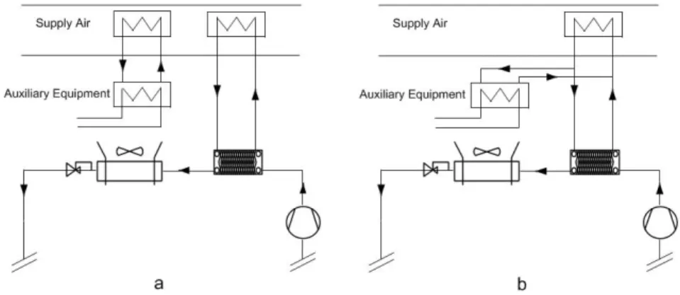
Recovered heat is used as well for space heating or fulfilling the demand in ventilation system. Different corresponding system layouts are shown in Figure 8. Refrigeration system can be connected to the heat
exchanger in ventilation system by indirect circuit or either by a heat exchanger locating before gas cooler known as de-superheater. Figure 8-a shows option using indirect system. Coolant fluid gains heat in condenser and releases it to HVAC system. The rest of heat is rejected to ambient and the temperature of coolant fluid from heating system is lowered. This option is mostly used for conventional HFC refrigerants with low discharge temperature (Sawalha, 2013). Figure 8-b shows another solution recovering heat via de-superheater. In this solution, the refrigerants with high discharge temperature such as CO2 or
NH3 should be used to increase the heat recovery efficiency. In case of ventilation system failure, alternative heating equipment like auxiliary electrical heater or another heat exchanger transferring heat from district heating or heat pump is utilized. Alternative equipment can be linked to ventilation system separately or in the same loop as refrigeration system depicted in Figure 9(a-b). (Arias, 2005)
Figure 8 - Heat recovery solutions connected to heating system
Figure 9 - Parallel heating equipment connected in different ways to heating system
2.6 CO2 heat recovery analysis
Raising the pressure is known as major strategy for making more heat available for recovery. By increasing the discharge pressure, the compressor outlet temperature reaches higher degree. The return temperature from heating system which is the water inlet to de-superheater is also important parameter in recovering heat. It is important that the return water would be as low as possible; the lower return temperature more heat can be recovered. It is difficult to achieve low return temperature in current heating systems. In practice, 30 ℃ is good return temperature meaning the heating system is efficient. Figure 10shows the amount of available heat for recovery in de-superheater for CO2 with exit temperature of 35 degree out of
de-superheater without any sub-cooling in subcritical region. In sub-critical area, condensation is done by gas cooler and major share of heat which is not possible to be recovered is rejected to the ambient. In trans-critical area, de-superheater can work with full capacity and all the heat down to 35 degree can be
recovered. Around transition area from sub-critical to trans-critical, slight increase in condensing pressure results in large amount of available heat thank to special shape of isotherms line in trans-critical area.
Figure 10 - PH diagram of CO2 for different discharge pressure 2.6.1 Optimum discharge pressure
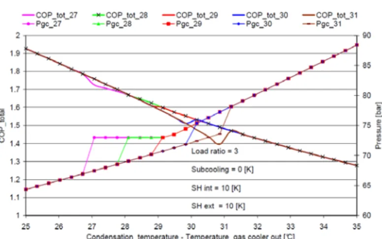
As the pressure is increased just upon the critical point, both compressor work and cooling capacity increase but the effect of cooling capacity increase is more dominant resulting in better performance of the system. After some range of pressure, slope of isotherm lines get steep which causes sharp drop in COP of system. So, for each isotherm line there should be an optimum pressure which system could be operated at.
Above the critical point, pressure and temperature are independent of each other. Discharge pressure could be adjusted based on gas cooler exit temperature of CO2 which is dependent on ambient
temperature considering specific degree of approach difference at gas cooler exit. Sawalha(2008) investigates the optimum operating discharge pressure of the system for achieving maximum COP. Gas cooler exit temperature is determined based on ambient temperature with using 5K approach difference expressed by equation(1). Figure 11 shows the cooling COP of refrigeration system for different gas cooler exit temperature. The optimum values for COP were curve fitted and the equation(2)is gained based on the gas cooler exit temperature.
𝐓𝐠𝐜,𝐞𝐱𝐢𝐭= 𝐓𝐚𝐦𝐛𝐢𝐞𝐧𝐭+ ∆𝐓𝐠𝐜,𝐚𝐩𝐩𝐫𝐨𝐚𝐜𝐡 Equation 1
𝐏𝐎𝐩𝐭𝐢𝐦𝐮𝐦= 𝟐. 𝟕 x 𝐓𝐠𝐜,𝐞𝐱𝐢𝐭− 𝟔. 𝟏 Equation 2 Optimum pressure based on gas cooler exit temperature is obtained for achieving highest cooling COP of
the system in trans-critical area. In order to derive the optimum operating pressure when the system is used for heat recovery, de-superheater exit temperature should be used instead expressed in equation (3). Necessarily it does not mean that the system should always be operated at this pressure to recover heat at maximum COP, but it means this pressure is the maximum pressure which system can be operated at in heat recovery mode. If the pressure rises higher than this pressure, recovered amount of heat is not beneficial respect to net given work to the system for heat recovery purpose. The pressure should be adjusted to fulfill the heating demand up to maximum operating pressure and then rising the discharge pressure is not suitable strategy for increasing the heat recovery potential in the system.
Figure 11 - Cooling COP VS discharge pressure for different gas cooler outlet temperature (Sawalha, 2008)
This equation is derived for trans-critical area and for temperature lower than 29.3 ℃ it gives a pressure which is lower than critical point. The range of pressure just below the critical point should be avoided in the system operation. Figure 12 shows the cooling COP versus condensation temperature for different return temperatures regarding no sub-cooling in the system. Below the critical point cooling COP has a sharp drop sine discharge pressure is increasing while cooling capacity reduces. For this range of condensation temperature, it is proposed to increase the pressure up to slightly higher than critical point. In this case, cooling capacity and capacity available for heat recovery increase considerably while condensing pressure is raised slightly.
𝐏𝐌𝐚𝐱𝐢𝐦𝐮𝐦 𝐨𝐩𝐞𝐫𝐚𝐭𝐢𝐧𝐠= 𝟐.𝟕 x 𝐓𝐝𝐞𝐬𝐮𝐩𝐞𝐫𝐡𝐞𝐚𝐭𝐞𝐫 𝐞𝐱𝐢𝐭− 𝟔. 𝟏 Equation 3
Figure 12 – Cooling COP VS condensation temperature for different return temperature (Frelechox, 2009)
Above the critical point pressure is determined based on the optimum pressure equation and in sub-critical area pressure and condensation temperature are dependent on each other. In sub-sub-critical section, Frelechox(2009) proposes that condensing pressure should be elevated to 74 Bar in advance for every gas cooler outlet temperature even if this pressure is higher than what is required meet the demand. In this way a smoother line for COP is achieved and major reduction in both cooling and heating COP can be avoided.
In heat recovery mode when the de-superheater exit temperature which depends on the return temperature of water from heating system is reached to 27C, condensing pressure should be increased a little bit higher above the critical point. If the refrigeration system is operating with no sub-cooling, this measure can also improve cooling COP of the system at the same time.
2.7 Heat recovery control strategy
Sawalha(2012) investigates theoretically heat recovery in CO2 trans-critical booster refrigeration system.
Discharge pressure of compressor is studied not as the only parameter affecting the heat recovery but also the effect of sub-cooling as affecting parameter on the system performance is evaluated.
Heat recovery ratio which is defined as the ratio of heat demand to cooling capacity in medium temperature level including freezing capacity and low stage compressor work is used as indicator of heat demand. Heat recovery ratio is a non-dimensional number which can be considered as parameter to compare the rate of heat recovery in different supermarkets with different solutions and various sizes. Heat recovery ratio and cooling capacity at medium temperature definitions are expressed in equation (4-5):
𝐇𝐑𝐑 = 𝐐𝐝𝐞𝐬𝐮𝐩𝐞𝐫𝐡𝐞𝐚𝐭𝐞𝐫
𝐐𝐦,𝐭𝐨𝐭𝐚𝐥 Equation 4
𝐐𝐦,𝐭𝐨𝐭𝐚𝐥= 𝐐𝐦,𝐜𝐚𝐛𝐢𝐧𝐞𝐭+ 𝐐𝐟,𝐜𝐚𝐛𝐢𝐧𝐞𝐭+ 𝐄𝐟,𝐬𝐡𝐚𝐟𝐭 Equation 5
Figure 13 - Controlled discharge pressure and gas cooler exit temperature VS heat recovery ratio (Sawalha, 2013)
Increasing sub-cooling in the gas cooler improves cooling COP of the system whereas it causes reduction in available heat in the system at the same time. Higher sub-cooling in the system reduces mass flow which decreases available heating energy in the system. Sawalha(2013) proposes adjusting discharge pressure to cover heating demand up to optimum operating discharge pressure which corresponds to de-superheater exit temperature. On the other hand highest possible sub-cooling should be maintained and the CO2 temperature before entering expansion valve should be lowered as much as possible. In another
word, heat demand should be met with raising the pressure and gas cooler should work with full capacity to maintain maximum amount of sub-cooling. The positive effect of sub-cooling on the cooling COP will be more dominant than the effect of work increase due to pressure raise. Then if the system has reached its optimum operating pressure while the heating load is not fulfilled, the pressure should be kept and gas cooler capacity should be reduced to decrease sub-cooling. Reduction in sub-cooling increases mass flow rate in the system enabling the system to recover more heat in de-superheater. Above the optimum pressure, the effect of reducing sub-cooling is less negative compared to increasing pressure. Figure 13 shows the operating discharge pressure and gas cooler exit temperature for controlled condition for de-superheater exit temperature of 35℃.
2.8 COP definition
Efficiency of the refrigeration system and associated heat recovery is very dependent on how the coefficient of performance for both refrigeration and heat recovery is defined. For booster trans-critical system, Gavarrel (2011) defines the coefficient of performance for low and medium temperature levels shown in equation (6-8) for CO2 booster refrigeration system. At each level to get the cooling COP,
cooling capacity at each level is divided by the corresponding compressor work. In booster systems, mass flow in low temperature level is mixed with mass flow in medium level after compression in low stage and compressed up to condensing level by high stage compressor. Thus, there is a share in high stage compressor work dedicated to compression of low level mass flow. This share should be extracted from high stage compressor work in calculation of medium level COP. On the other hand, in calculation of freezing level, this share should be added to low stage compressor work. Gavarrel (2011) proposes to calculate this share based on the fraction of freezer cooling to the total cooling shown in equation (8). 𝐂𝐎𝐏𝐌𝐓= 𝐄𝐌𝐒𝐐−𝐄𝐌𝐓𝐌𝐒,𝐟 Equation 6 𝐂𝐎𝐏𝐋𝐓= 𝐄 𝐐𝐋𝐓
𝐋𝐒+𝐄𝐌𝐒,𝐟 Equation 7
𝐄𝐌𝐒,𝐟= 𝐄𝐌𝐒× 𝐐𝐋𝐓𝐐+𝐐𝐌𝐓𝐌𝐓 Equation 8 Kristensen et al. (2013) considers the effect of freezer mass flow compressed by high stage compressor in COP calculation but defines the COP correlations in a different way shown in equation(9-12). fLS and fMS are fraction of low stage and medium stage work to the total work.
𝐂𝐎𝐏𝟐,𝐟= 𝐄𝐋𝐒+𝐟𝐐𝐋𝐓𝐋𝐒𝐄𝐇𝐒 Equation 9 𝐂𝐎𝐏𝟐= 𝐟𝐌𝐒𝐐𝐌𝐓𝐄𝐌𝐒 Equation 10 𝐟𝐋𝐒 = 𝐄𝐋𝐒𝐄+𝐄𝐋𝐒𝐇𝐒 Equation 11 𝐟𝐌𝐒 = 𝐄𝐋𝐒𝐄+𝐄𝐇𝐒𝐇𝐒 Equation 12 Total cooling COP is defined mostly as the ratio of total cooling to the total work given to the compressors shown in equation (13).
𝐂𝐎𝐏𝟐= 𝐐𝐄𝐋𝐓𝐋𝐒+𝐄+𝐐𝐌𝐓𝐌𝐓 Equation 13 In the refrigeration systems with heat recovery, global COP or total coefficient of performance is used to give a general efficiency of system. Tambotsev et al (2011), Reinholdt et al (2012) and Kristensen et al define the total coefficient of performance as the ratio of whatever is gained in both cooling and heating side to the total work given to the compressor in freezing and intermediate level shown in equation (14). In case of refrigeration system failure to cover the heating demand, parallel heating system is required. Denecke (2012)suggests to add the work required in supplementary equipment to the compressor work expressed in equation (15). Usually electrical heater or heat pump is being used if refrigeration system would not be able to cover the demand.
𝐂𝐎𝐒𝐏 = 𝐐𝐋𝐓+𝐐𝐌𝐓+𝐐𝐇𝐑
𝐄𝐋𝐒+𝐄𝐌𝐒 Equation 14
𝐂𝐎𝐒𝐏 = 𝐐𝐋𝐓+𝐐𝐌𝐓+𝐐𝐇𝐑
𝐄𝐋𝐒+𝐄𝐌𝐒+𝐏𝐄𝐥 Equation 15
Tambovtsev et al (2011) defines the heat recovery coefficient of performance as the ratio between amount of recovered heat and total compressor power shown in equation (16). The compressor work is whatever used for covering the cooling demand and meeting the heat load. But Sawalha (2013) and Reinholdt et al. (2012) suggest a more indicative definition shown in equation (17) excluding the share of compressor work which is related to fulfilling the cooling demand. In another word, the share of work which is resulted by shifting the pressure to recover required amount of heat is included as compressor work for heat recovery purpose. In this case, the net COP of heat recovery can be compared to the COP of heat pump or any other parallel heating system which is utilized to meet the heat demand. In this thesis the COP definition of Sawalha (2013) is used to evaluate the system efficiency in heat recovery mode.
𝐂𝐎𝐏𝐇𝐑= 𝐐𝐄𝐇𝐑𝐇𝐑 Equation 16 𝐂𝐎𝐏𝐇𝐑= 𝐄𝐇𝐑𝐐𝐇𝐑−𝐄𝐅𝐂 Equation 17
3 MASS FLOW RATE CALCULATION ANLYSIS
3.1 Mass Flow estimation method
Mass flow in refrigeration systems is an essential parameter to understand the behavior of system and evaluate its efficiency. Direct measurement of mass flow rate in the supermarket is not possible since the mass flow meter price is extremely high and installing such a device is not preferable. Thus, the mass flow rate should be estimated indirectly. There are many indirect method such as Dabiri’s method (1981) volumetric efficiency, total efficiency, y-method (Gimenez,2011) and heat balance method. In this section it is tried to describe briefly three methods indirect mass flow rate estimation.
3.1.1 Volumetric method
This method is based on volumetric efficiency definition expressed in equation (18):
𝛈𝐯= 𝐕𝐦𝐜𝛒 Equation 18 Where:
ηv is volumetric efficiency
m is mass flow rate of refrigerant (kg
s)
Vc is volumetric flow rate (ms3) ρ is density (kg
m3)
Volumetric efficiency can be extracted directly from compressor data which is based on the empirical tests done by the company manufacturer. The great advantage of this method is that it is independent of compressor condition and heat dissipation from compressor to the ambient in machine room. The surrounding temperature might be fluctuating during different period of times affecting the heat loss from the compressor. Furthermore the correlation for volumetric efficiency gives high compatibility with pressure ratio resulting in high accuracy. But the big disadvantage of this method is that depending on the number of compressors running in the system, the swept volume used in the equation varies. Since it is not clear how many compressors are running at the moment, it is tough to use this method for long periods. Number of the compressors can be estimated using the electric power consumption of all the compressors. However the number of compressor is not the only parameter affecting the power of compressor, but also the pressure ratio depending on condensing and evaporating pressure and the amount of superheat are other effective parameters. (Gimenez, 2011)
3.1.2 Total efficiency method
This solution uses the total efficiency of the compressor stated in equation(19): 𝛈𝐓𝐨𝐭𝐚𝐥= 𝐦 ∆𝐡𝐢𝐬
𝐄 Equation 19
Where:
ηTotalis total efficiency
m is mass flow rate of refrigerant (kg s)
∆hisis isentropic enthalpy difference over the compressor (kgkJ)
Ė is the electrical compressor power (kW)
This method uses the inlet condition of refrigerant and isentropic enthalpy difference over the compressor. This method can be used regardless of the number of the compressor and it only needs the power inlet to the compressor which is a very important benefit. Total efficiency is derived from manufacturer company data sheet. Compared to volumetric efficiency, the total efficiency is more scattered giving slightly lower accuracy. (Gimenez, 2011)
3.1.3 Heat balance method
Heat balance proposes another method for mass flow rate estimation. In this method shown by equation (20), mass flow is calculated by dividing input power to the refrigerant by the actual enthalpy difference over the compressor. Input power to the refrigerant is estimated by extracting compressor heat loss from electrical input power. Heat loss from the compressor is assumed to be 7 % of input power (Berglöf, 2010) and electrical efficiency is considered to be 95 %. (Karampour, 2011)
𝐦 = 𝛈𝐞𝐥𝐡𝐄𝐞𝐥−𝐐𝐂𝐨𝐦𝐩𝐫𝐞𝐬𝐬𝐨𝐫 𝐥𝐨𝐬𝐬
𝐂𝐨𝐦𝐩 𝐎𝐮𝐭−𝐡𝐂𝐨𝐦𝐩 𝐈𝐧 Equation 20
Where:
ηel is electrical efficiency compressor
Eel is electrical power input
hComp In is the compressor inlet enthalpy
hComp Out is the compressor outlet enthalpy
3.2 Experimental analysis
Theoretical estimation methods explained previously are tested by experimental test rig existing in Energy technology department of KTH and accuracy of each method is investigated. The test rig and the running condition are described and the results are discussed in following sections.
3.2.1 Test rig description
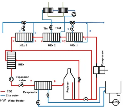
Test rig is located in the lab of applied thermodynamic and refrigeration at energy technology department of KTH shown in Figure 14. It is one single compression refrigeration cycle consisted of 5 main plate heat exchangers and one Dorin TCS362/4-D compressor. There is a receiver after evaporator accumulating CO2 as refrigerant. Three of plate heat exchangers are used as gas cooler cooled by water city. Two heat exchangers, 1st and 3rd ones, are linked together and cooled directly by city water. The 2nd heat exchanger
is linked to a closed loop connected indirectly to water city by two other heat exchangers. Internal heat exchanger is also designed in the test rig making extra sub-cooling by transferring heat from suction line. For expansion valve, electronic Danfoss valve is used. Ethylene glycol is used as brine stored in a tank close to test rig and heated up by a heater.
Temperature and pressure are measured by sensors used before and after all heat exchangers and compressor too. Coriolis mass flow meter (KCM600) is used to measure the mass flow rate of refrigerant.
Figure 14 - Schematic layout of test rig at Energy technology department of KTH
3.2.2 Methodology
The main aim of running the test rig is to check the other mass flow rate estimation methods and evaluate the accuracy of these methods. Only 1st and 2nd heat exchangers are used as gas cooler and 3rd heat
exchanger and internal heat exchanger have been off. At each running condition, it is tried to maintain the evaporation pressure at certain range (35-30bar) while the discharge pressure is varied by adjusting expansion valve opening degree and speed of compressor. The lowest opening degree of expansion valve is set to 7% open and the speed of compressor is varied between 1050-1800 rpm. The heater is switched on 2-3 hours before each running condition in order to increase the heat source temperature and have enough heat capacity over the evaporator to prevent evaporation temperature drop.
For each new testing condition, the system is let to reach the steady state condition and data is retrieved. Beside the direct measurement of mas flow rate by coriolis mass flow meter, three other methods of volumetric efficiency, total efficiency and heat balance are used to calculate the mass flow and the accuracy of each method is evaluated.
3.2.3 Results & Discussion
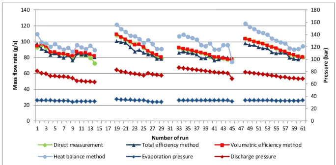
The test rig is run for different conditions. Figure 15 shows the evaporation and discharge pressure for all the running conditions. Discharge pressure varies between 85-60 bar while the evaporation temperature is fixed at 33bar. Results for direct measurement and also three methods of total efficiency, volumetric efficiency and heat balance method are expressed by Figure 15-16. Volumetric efficiency method result almost overlaps the direct measurement result and shows very good matching. Compared to volumetric efficiency, total efficiency lies below the direct measurement and shows lower accuracy. Results from heat balance methods shows the biggest gap located far away from measured number. Percentage of error for three methods can be seen in Figure 16. Volumetric method has the lowest error which is around 2-3 %. Total efficiency method is the next accurate method with maximum accuracy of 10%. Heat balance method is the worst mass flow rate estimating method with highest accuracy reaching 20 %. It shows that the assumption for heat loss from compressor used in calculation should be reconsidered.
In this thesis total efficiency method is used for mass flow rate calculations. According to the experimental results volumetric method has the highest accuracy but in field measurement analysis it is so impossible to use. In this method, it is essential to know the compression volume and subsequently the number of cylinders in each compressor while such data is missing from field measurement.
Figure 15 - Mass flow rate for direct measurement and different estimation methods
Figure 16 - Accuracy of different mass flow rate estimation methods
0 20 40 60 80 100 120 140 160 180 0 20 40 60 80 100 120 140 1 3 5 7 9 11 13 15 17 19 21 23 25 27 29 31 33 35 37 39 41 43 45 47 49 51 53 55 57 59 61 Pr es sur e ( ba r) M as s f lo w rat e (g /s ) Number of run
Direct measurement Total efficiency method Volumetric efficiency method Heat balance method Evaporation pressure Discharge pressure
0 10 20 30 40 50 60 70 80 90 100 1 3 5 7 9 11 13 15 17 19 21 23 25 27 29 31 33 35 37 39 41 43 45 47 49 51 53 55 57 59 61 Er ro r ( % ) Number of run
Total efficiency method Volumetric efficiency method Heat balance method
4 FIELD MEASUREMENT ANALYSIS
4.1 Description of supermarkets refrigeration system
In this section, refrigeration and heating system for two existing supermarkets are described. The refrigeration system in both supermarkets is CO2-booster type. The 1st supermarket called TR2 is located in Hovås in south of Sweden and the 2nd supermarket, TR3 is located in Piteå in north of Sweden.
4.1.1 TR2
Figure 17 shows the total layout of TR2 including heated space where the cabinets and products are located, refrigeration system and heat pump which is used as parallel heating system.
Figure 17 - Schematic layout of TR2 supermarket
In this supermarket, refrigeration system is consisted of three units. Both units of KAFA1 and KAFA2 are booster units each having two pressure levels for cooling and freezing. Heat recovery in this system is done by de-superheater which is supplying heat to ventilation system. The rest of heat is dumped to ambient by gas cooler. In this system before the expansion valve, extra sub-cooling after the gas cooler is done by the borehole connected to heat pump.
Figure 18 - Schematic layout of refrigeration system at TR2
Beside KAFA1 and KAFA2 there is another parallel unit consisted of only medium temperature level which is called KA3. Figure 18 shows schematic layout for KAFA2 and KA3 connected to heating system. The same as two other units, heat is recovered in the desuperheater and the rest is dissipated to ambient by gas cooler. Similar to other units it is connected to borehole to make extra subcooling before the expansion valve inlet.
Figure 19 - Measurement layout of refrigeration system at TR2
Figure 19, shows the temperature and pressure measurements for unit KAFA1. After and before the compressors and heat exchanger, pressure and temperature are measured. Only temperature of CO2 after the gas cooler is missing which is an important measurement since it gives critical understanding of subcooling level done by gas cooler itself. Figure 20 shows the connections of all three units to gas cooler on the roof, to the borehole and to the ventilation system. The heated water mixture from all three units goes to heating system. Unfortunately the measurement on heating system is not available which makes the calculation of total heating demand impossible.
Figure 20 - Measurement layout of water at TR2
4.1.2 TR3
This system is consisted of two booster units KAFA1 and KAFA2. The simple schematic layout of refrigeration system is shown in Figure 21. The same as TR2, the heat recovery is done by de-superheater before the gas cooler. Unlike TR3 this system is not connected to borehole and for making sub-cooling, gas cooler works at higher capacity to provide enough sub-cooling.
Figure 22 show the different measurements in unit KAFA1. In this case, all the parameters are accessible. Figure 23 the refrigeration system connected to ventilation system. Beside the recovered heat from refrigeration system, district heating is used as supplementary heating system connected to ventilation system directly and indirectly. Since the amount of heat from district heating is not available due to lack of measurement on heating system, it is not possible to estimate the share of refrigeration system in meeting the total heating demand in the building.
Figure 21 - Schematic layout of refrigeration system at TR3
Figure 22 - Measurement layout of refrigeration system at TR3
Figure 23 - Measurement layout of water at TR3
4.1.3 Data retrieval
Data for two refrigeration systems, TR2 and TR3 is gained through IWMAC interface. Two systems are evaluated from heat recovery point of view for two continuous years of 2011 and 2012. In IWMAC interface, the value for each parameter is not measured simultaneously with other parameters and also the time interval for one parameter during specific period is not constant. In order synchronize the measured values with even time interval, an excel macro created by Vincent Cottineau (2011) is used. By this excel macro the time interval is chosen to be 10 minute meaning the data is averaged during each 10 minutes.
4.2 COP calculation analysis
Cooling capacity in low and medium temperature is calculated using equation (21-22) respectively. Mass flow rate for low temperature level is obtained by making an energy balance over the low stage compressor using total efficiency of the compressor and inlet conditions to the compressor. Total mass flow rate is calculated by the same method for high stage compressor. In order to calculate the cooling capacity in medium temperature level, the total mass flow is used but the share of cooling capacity in low
stage compressor is withdrew. A part of electrical work into the compressor is wasted to ambient which is considered to be 7 % (Berglöf, 2010).
𝐐𝐋𝐓 = 𝐦(𝐡𝐄𝐯𝐚𝐩 −𝐋𝐓−𝐎𝐮𝐭− 𝐡𝐄𝐯𝐚𝐩 −𝐈𝐧) Equation 21
𝐐𝐌𝐓= 𝐦�𝐡𝐄𝐯𝐚𝐩−𝐌𝐓−𝐎𝐮𝐭− 𝐡𝐄𝐯𝐚𝐩 −𝐈𝐧� − 𝐐𝐋𝐓− 𝐄𝐋𝐒∗ (𝟏 − 𝐇𝐞𝐚𝐭 𝐋𝐨𝐬𝐬 𝐢𝐧 𝐋𝐒 𝐂𝐨𝐦𝐩) Equation 22
Where:
QFreezing is cooling capacity in low temperature level
QCooling,MT is cooling capacity in medium temperature cabinets mf is mass flow rate in low stage compressor
m is mass flow rate in high stage compressor hEvap−In is refrigerant enthalpy at evaporator inlet
hEvap−LT−Out is refrigerant enthalpy at the low temperature evaporator exit hEvap−MT−Out is refrigerant enthalpy at the Medium temperature evaporator exit ELS is low stage compressor work
The recovered heat in de-superheater is calculated by multiplying total mass flow rate with enthalpy difference of refrigerant over de-superheater shown by equation (23). With the same manner, dissipated heat in gas cooler is expressed by equation (24).
𝐐𝐇𝐑= 𝐦�𝐡𝐃𝐢𝐬𝐜𝐡𝐚𝐫𝐠𝐞− 𝐡𝐃𝐞𝐬𝐮𝐩𝐞𝐫𝐡𝐞𝐚𝐭𝐞𝐫 −𝐎𝐮𝐭 � Equation 23
𝐐𝐆𝐂= 𝐦�𝐡𝐃𝐞𝐬𝐮𝐩𝐞𝐫𝐡𝐞𝐚𝐭𝐞𝐫−𝐎𝐮𝐭 − 𝐡𝐆𝐚𝐬 𝐜𝐨𝐨𝐥𝐞𝐫−𝐎𝐮𝐭 � Equation 24
Where:
QRecovered Heat is recovered heat in des-uperheater QReleased Heat is released heat in gas cooler
hDischarge is refrigerant enthalpy at compressor outlet
hDesuperheater−Out is refrigerant enthalpy at desuperheater outlet hGas cooler−Out is refrigerant enthalpy at gas cooler exit
COP calculation freezing and medium temperature level is shown in equation (25-26). For freezing COP, the share of work in medium temperature corresponding to freezer is added to low stage work. For medium temperature level the cooling capacity in both low and high stage plus work given in to refrigerant in low stage is divided by work in high stage compressor.
𝐂𝐎𝐏𝐋𝐓 = E 𝐐𝐋𝐓
𝐌𝐒−𝐂𝐎𝐏𝐌𝐓𝐐𝐌𝐓+E𝐋𝐒 Equation 25 𝐂𝐎𝐏𝐌𝐓= 𝐐𝐋𝐓+𝐐𝐌𝐓+E𝐋𝐒∗(𝟏−𝐇𝐞𝐚𝐭 𝐋𝐨𝐬𝐬 𝐢𝐧 𝐋𝐒 𝐂𝐨𝐦𝐩 )E𝐌𝐒 Equation 26
4.3 Control strategies for supermarket refrigeration systems
System behavior for TR2 and TR3 are calculated for yearly, monthly and daily periods. The variation in important parameters such as discharge pressure and gas cooler exit temperature is scrutinized and the effect on cooling and heating capacity is evaluated.
4.3.1 Yearly analysis
To have general understanding about system operation, cooling and heating capacity yearly view is studied in the beginning. The behavior of system is monitored for 2012 in monthly averaged values for TR2 and TR3.
4.3.1.1 TR2
Figure 24 shows the monthly values for discharge pressure, condensation temperature, expansion valve inlet temperature and ambient temperature for 2012 for KAFA1 unit in TR2. For the warm season which there is no need for heat recovery, the system is run in floating condensing mode. From May until September discharge pressure follows the ambient temperature. In cold season the discharge pressure is raised to some extent to fulfill the heat demand in the building. The monthly average discharge pressure is under critical point and refrigeration system is not run in trans-critical area. Within heat recovery period, the refrigerant coming out of gas cooler is sub-cooled by borehole down to 5 ℃. At this time the difference between saturation temperature and expansion valve inlet temperature is rather high showing high degree of sub-cooling in cold months. But as expansion valve inlet temperature overlaps with saturation temperature in warm season specifically during July and August, borehole is bypassed and no sub-cooling is done.
Figure 24 - Monthly averaged measured values at TR2 - 2012
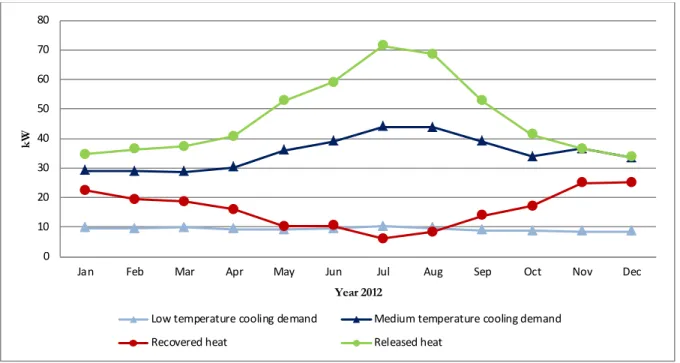
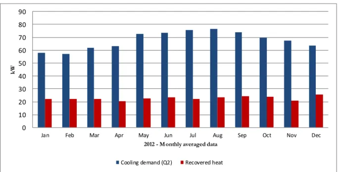
Cooling demands at low and medium temperature levels, heat recovery rate and released heat are shown in Figure 25 in hourly averaged values. Low temperature cooling demand is constant and stable regardless of ambient temperature during the whole year but cooling demand increases in summer due to higher air humidity in summer. The heat recovery rate is constant for the both cold and warm period. During summer, because of warm ambient temperature system is run in floating condensing mode with rather high discharge pressure. Regarding the high mass flow rate of the system which is due to high cooling demand in summer, the system is able to recover considerable amount of heat for such mild weather. In winter time, as explained previously discharge pressure is raised to do heat recovery but respect to high heat demand of the building in winter, low level of heat is recovered and system is not run in trans-critical region meaning low potential of heat recovery in the refrigeration system is used. Refrigeration system has covered small share of total heat demand and the major part is covered by heat pump as parallel system existing in the supermarket.
0 10 20 30 40 50 60 70 80 -10 0 10 20 30 40 50 60
Jan Feb Mar Apr May Jun Jul Aug Sep Oct Nov Dec
Pre ss ure ( ba r) T em pe ra tu re (c) Year 2012
Ambient temperature Gas cooler exit temperature Expansion valve inlet temperature Discharge pressure
Figure 25 - Monthly averaged cooling demands and recovered heat at TR2 – 2012
4.3.1.2 TR3
The same yearly analysis shown in Figure 26-27is done for TR3 supermarket. Figure 26 shows discharge pressure, gas cooler exit temperature and ambient temperature in monthly averaged values. Discharge pressure is controlled in the same manner as TR2 during 2012; in summer time discharge pressure follows the ambient temperature and system is run in floating condensing mode but in winter time the pressure is shifted up. At the end of the year, in 2012 the average discharge pressure for December reaches to critical point indicating higher level of heat recovery than TR2. In this system there is no borehole and sub-cooling is done by gas cooler itself. In winter time, specifically in January and February there is still some possibility to have higher degree of sub-cooling by regulating the gas cooler in a better way. However it is not possible to reduce the gas cooler exit temperature lower than specific level due to technical problems. In December despite of very low ambient temperature, gas cooler exit temperature is maintained at lowest possible value which is close 0℃. Within the warm period, gas cooler exit temperature follows the ambient temperature with approach difference 5 degree at the gas cooler outlet.
Figure 26 - Monthly averaged measured values at TR3 - 2012
0 10 20 30 40 50 60 70 80 90 100
Jan Feb Mar Apr May Jun Jul Aug Sep Oct Nov Dec
kW
Year 2012
Low temperature cooling demand Recovered heat
Released Heat Medium temperature cooling demand
0 10 20 30 40 50 60 70 80 -15 -5 5 15 25 35 45 55
Jan Feb Mar Apr May Jun Jul Aug Sep Oct Nov Dec
Pre ss ure (b ar) T em pe ra tu re (C ) Year 2012
Ambient temperture Gas cooler exit temperature Discharge pressure