THESIS
ADAPTIVE SPATIOTEMPORAL DATA INTEGRATION USING DISTRIBUTED QUERY RELAXATION OVER HETEROGENEOUS OBSERVATIONAL DATASETS
Submitted by Saptashwa Mitra
Department of Computer Science
In partial fulfillment of the requirements For the Degree of Master of Science
Colorado State University Fort Collins, Colorado
Summer 2018
Master’s Committee:
Advisor: Sangmi Lee Pallickara Shrideep Pallickara
Copyright by Saptashwa Mitra 2018 All Rights Reserved
ABSTRACT
ADAPTIVE SPATIOTEMPORAL DATA INTEGRATION USING DISTRIBUTED QUERY RELAXATION OVER HETEROGENEOUS OBSERVATIONAL DATASETS
Combining data from disparate sources enhances the opportunity to explore different aspects of the phenomena under consideration. However, there are several challenges in doing so effectively that include inter alia, the heterogeneity in data representation and format, collection patterns, and integration of foreign data attributes in a ready-to-use condition. In this study, we propose a scalable query-oriented data integration framework that provides estimations for spatiotemporally aligned data points. We have designed Confluence, a distributed data integration framework that dynamically generates accurate interpolations for the targeted spatiotemporal scopes along with an estimate of the uncertainty involved with such estimation. Confluence orchestrates computations to evaluate spatial and temporal query joins and to interpolate values. Our methodology facilitates distributed query evaluations with a dynamic relaxation of query constraints. Query evaluations are locality-aware and we leverage model-based dynamic parameter selection to provide accurate estimation for data points. We have included empirical benchmarks that profile the suitability of our approach in terms of accuracy, latency, and throughput at scale.
ACKNOWLEDGEMENTS
First and foremost, I would like to thank my parents, Sumita and Subrata Mitra, for being my pillars of support and strength throughout my life. I thank them for showering me with uncondi-tional love and always believing in me and pushing me to do better. Thank you, for all the sacrifices you have made, both in your life and your career to ensure that I always had the best opportunities in life.
I would also like to thank my advisor Dr. Sangmi Lee Pallickara for her guidance. Research was (and is still) not easy for me and I thank her for being patient with me, providing valuable advice and for her continued support throughout my career here at CSU.
I thank my committee members, Dr. Shrideep Pallickara and Dr. Kaigang Li, for promptly agreeing to be on my Thesis committee. Thank you for accommodating my Thesis defense on a such a short notice and for your valuable inputs. My research has been supported by funding from the US National Science Foundations Advanced Cyberinfrastructure (ACI-1553685), so I am grateful to them for their financial support.
Finally, I would like to thank all the faculty and staff here at the Computer Science Department for being so helpful and making life at the university pleasant.
TABLE OF CONTENTS
ABSTRACT . . . ii
ACKNOWLEDGEMENTS . . . iii
LIST OF TABLES . . . vii
LIST OF FIGURES . . . viii
Chapter 1 Introduction . . . 1
1.1 Research Questions . . . 2
1.2 Overview of Our Approach . . . 2
1.3 Paper Contributions . . . 3
1.4 Paper Organization . . . 4
Chapter 2 Background and Related Work . . . 5
2.1 Related Work . . . 5
2.1.1 Spatiotemporal Data Analysis . . . 5
2.1.2 Spatiotemporal Interpolation . . . 7
2.2 Spatiotemporal Data Integration . . . 8
2.3 Distributed Geospatial Data Storage System . . . 9
2.3.1 Galileo Cluster Structure . . . 9
2.3.2 Galileo Metadata Graph . . . 10
2.4 Candidate Dataset Properties . . . 11
Chapter 3 Relaxed Geospatial Join Across Geospatial Data Representation Models . . . 13
3.1 Relaxed Conditions for Data Integration . . . 13
3.2 Self-Adaptive Relaxation Conditions . . . 15
Chapter 4 Methodology . . . 17
4.1 Distributed Query Relaxation . . . 17
4.2 Relaxation Region . . . 18
4.2.1 Neighboring Blocks . . . 18
4.2.2 Maximum Spatial and Temporal Relaxation . . . 19
4.2.3 Maximum Relaxation Region (MRR) . . . 20
4.2.4 Bordering Region . . . 20
4.2.5 Neighbors0Orientation . . . 21
4.3 Spatiotemporal Border Indexing Scheme . . . 22
4.3.1 Border Index Overview . . . 22
4.3.2 Border Index Components . . . 23
4.3.3 Figuring out Orientation . . . 24
4.3.4 Neighbor Elimination Using Bordering Index . . . 24
4.3.5 Partial Block Processing Using Bordering Index . . . 26
4.4 Feature Interpolation With Uncertainty . . . 27
4.4.2 Vector-to-Raster/ Raster-to-Vector . . . 29
4.4.3 Raster-to-Raster Interpolation . . . 30
4.5 Self-Adaptive Relaxation Conditions . . . 30
4.5.1 Training Data Generation . . . 32
4.5.2 Modelling β Value . . . 32
4.5.3 Dynamic β Prediction . . . 33
Chapter 5 System Architecture . . . 34
5.1 Effective Data Integration . . . 34
5.1.1 Minimizing Data Movement . . . 35
5.1.2 Chunkified/Segmented Integration . . . 36
5.1.3 Minimizing Block Reading . . . 37
5.1.4 Fast Record Merging . . . 38
5.2 Relaxed Data Integration Query . . . 39
5.2.1 Data Integration Request . . . 39
5.2.2 Data Integration Event . . . 40
5.2.3 Neighbor Data Request . . . 41
5.2.4 Neighbor Data Response . . . 41
5.2.5 Data Integration Response . . . 43
5.3 Generating Training Data for Neural Network Model . . . 44
5.3.1 Training Data Request . . . 44
5.3.2 Survey request . . . 44
5.3.3 Survey Response . . . 45
5.3.4 Training Data Event . . . 45
5.3.5 Training Data Response . . . 45
Chapter 6 System Evaluation . . . 46
6.1 Experimental Setup . . . 46
6.1.1 Distributed Cluster Configuration . . . 46
6.1.2 Training and Testing of Predictive Models for Interpolation Parameters . 46 6.1.3 Datasets . . . 47
6.2 Data Integration Latency Test . . . 48
6.2.1 Using Fixed β . . . 49
6.2.2 Using Dynamic β . . . 51
6.2.3 Vector-to-Raster Latency . . . 51
6.3 Data Integration Throughput Test . . . 52
6.4 Model Training and Accuracy . . . 53
6.4.1 Model Building Time . . . 53
6.4.2 Model Accuracy . . . 54
6.5 Resource Utilization . . . 54
6.6 Case Study - Obesity Prediction Using Integrated Data . . . 56
6.6.1 Problem Description . . . 56
6.6.2 Overview of Approach . . . 57
6.6.3 Target Variable . . . 58
6.6.5 Distributed Computing Environment . . . 59
6.6.6 Interpolation - Attribute based Uncertainty Estimation for Geospatial Data Integration . . . 59
6.6.7 Preliminary Analysis . . . 61
6.6.8 Integrating Datasets Based on Geospatial Proximity . . . 62
6.6.9 Data Pre-Processing and Feature Selection . . . 64
6.6.10 Estimating uncertainty . . . 64
6.6.11 Uncertainty Aware Modelling . . . 65
6.6.12 Experimental Evaluation . . . 66
6.6.13 Training and Testing of Predictive Models . . . 67
6.6.14 Scalability Evaluation . . . 67
6.6.15 Experimentation and Accuracy Evaluation . . . 68
Chapter 7 Conclusions . . . 72 7.1 Research Question 1(RQ1) . . . 72 7.2 Research Question 2(RQ2) . . . 72 7.3 Research Question 3(RQ3) . . . 72 7.4 Research Question 3(RQ4) . . . 73 Bibliography . . . 74
LIST OF TABLES
3.1 Relaxed Data Integration On Different Datasets . . . 15
6.1 RMSE for BMI predictions(for year 1997) using CDC Growth Chart . . . 62
6.2 Results from Feature Selection on Integrated Data . . . 69
LIST OF FIGURES
2.1 Node Partitioning Scheme . . . 10
2.2 Metadata Graph . . . 11
3.1 Relaxed Conditions(Geospatial) . . . 13
4.1 Relaxation Regions . . . 19
4.2 Border Flanks . . . 21
4.3 Neighboring Region Elimination: Scenario 1 . . . 25
4.4 Neighboring Region Elimination: Scenario 2 . . . 26
4.5 Partial Neighbor Block Processing . . . 27
5.1 MDC Algorithm for One Dimension . . . 38
5.2 Data Flow in Data Integration . . . 40
5.3 Process Flow in Data Integration . . . 43
6.1 Data Integration Latency With Fixed β . . . 50
6.2 Latency Breakdown . . . 50
6.3 Data Integration Latency With Dynamic β Prediction . . . 51
6.4 Data Integration Latency With Fixed β in Vector-to-Raster Scenario . . . 52
6.5 Throughput for Different Sizes of Query . . . 52
6.6 Model Building Time vs Training Data Size . . . 53
6.7 Accuracy Comparison - Dynamic β vs Fixed β . . . 55
6.8 CPU Utilizations . . . 55
6.9 CDC growth chart of BMI progression with age for American boys aged 2-20 years. . . 62
6.10 Strategy for merging Census 2000 & NLSY97 data . . . 63
6.11 Turnaround time with increasing cluster size . . . 67
6.12 Prediction RMSE with change in training data size for (a) Neural Network and (b) Gradient Boosting Models . . . 68
Chapter 1
Introduction
The rapid growth of geo-sensors and remote sensing technologies have allowed geoscientists to explore numerous and complex attributes to understand phenomena that evolve spatiotemporally. The collected data is often integrated with other datasets from different data sources to enhance exploration options. A starting point for such explorations is to use queries to retrieve relevant portions from disparate datasets. The results from these queries can then be fused to create a custom dataset.
Challenges in accomplishing this stem from data volumes, the characteristics of the dataset, and the data collection processed. Data generated by these sensors are voluminous and are produced at high velocities. The heterogeneity of the collected data including their resolutions, representations, and encoding format posed challenges in storing, retrieving, processing, and analyzing them. The data gathering process involves diverse sensing equipment and variations in the data collection patterns.
Existing frameworks for spatial data management [1–8] provide scalable solutions for geospa-tial data storing and query over the multiple datasets. While these systems are highly effective from the scalable storage system standpoint, their spatial join algorithms rely on traditional query evalu-ations that return intersecting polygon pairs that do not address the nature of mismatching between the locations of samples and timestamps. Once the data is retrieved, users perform data interpo-lations to estimate values at the precise matching location and time. This often causes repetitive data retrievals because most interpolation algorithms are iterative entailing access to the surround-ing area and/or temporal scopes. Furthermore, users often explore the parameters to achieve more accurate estimations.
To address these challenges, we propose a framework for accomplishing effective, accurate, and scalable data integration operations. In particular, our framework is independent of the under-lying data model and supports: (1) a distributed data hosting environment for the heterogeneous
datasets, (2) approximate join operations, (3) feature interpolations in case of spatiotemporal mis-alignment with uncertainty estimate, and (4) automatic interpolation parameter selection schemes.
1.1
Research Questions
Enabling scalable data integration operations over a distributed geospatial data storage must address challenges stemming from dataset sizes, variations in the density of data availability, and latency requirements during approximate query evaluation. The following research questions to guide our study in this paper:
• RQ1: How can we support query-based integration of diverse geospatial datasets that are not spatially and/or temporally aligned?
• RQ2 How can the system cope with different data representation models such as raster and vector?
• RQ3 How can we effectively orchestrate our data integration algorithm while ensuring sup-port for interactive applications?
• RQ4 How can the system select parameters of the interpolation algorithms that ensure the highest accuracy?
1.2
Overview of Our Approach
Our framework, Confluence, facilitates query-driven scalable and interactive spatiotemporal data integration. Confluence dynamically generates estimations at the aligned data point. Data alignments are performed based on the specified key indexing attributes such as spatial coordi-nates and temporal ranges. The integration operations support vector and raster data representation models. Raster data is made up of pixels (spatiotemporal extent) and each pixel has an associated value. Vector data model represents the data space using points, lines, and polygons. Our system automatically transforms values between models by means of aggregating data points or applying representative data values. The results are delivered with the associated uncertainty information.
Based on the user0s query (e.g. spatial coverage), the system performs distributed query relax-ation that allows query constraints to be relaxed to cover neighboring spatiotemporal scopes. The maximum range of relaxation is configurable in the system. To reduce data movements within the storage cluster, the system schedules the computations on nodes that host a majority of the data that match the user0s query. The system provides separate indexing schemes for boundary regions of blocks that need to be transferred to perform integration and it is used for query evaluation and caching.
This study proposes a dynamic relaxation model, an adaptive interpolation scheme to cope with the repetitive exploration of the parameter spaces for interpolation algorithms, such as In-verse Distance Weighing (IDW) [9]. Confluence trains model and estimates the best parameters for a given target spatiotemporal region. Our experiments used an artificial neural network to train the dynamic relaxation model for IDW, and it showed, depending on the feature being interpo-lated, an improvement in accuracy by 9% ∼ 31.25% with the estimation compared to using static parameters.
We validate our ideas in the context of the Galileo system for spatiotemporal data. Galileo is a cloud-compatible hierarchical distributed hash table (DHT) implementation for voluminous and multidimensional spatiotemporal observations [10]. The key organizing principle in Galileo is the use of geohashes whose precision can be controlled to collocate data from contiguous geographical extents.
1.3
Paper Contributions
Confluence targets interactive data integration that allows the analysis to import relevant por-tions of voluminous auxiliary dataset interactively. Our query-based data integration process per-forms dynamic alignments across datasets and also generates interpolated values in situations where data is unavailable. The dynamically generated estimations are ready-to-use as input to interactive analytics including visualizations. Specific contributions of Confluence include:
• A rapid, query-driven approach to data integration with dynamic, run-time estimation of values.
• A model-based approach to select the parameters that achieve the most accurate estimation per data points.
• Geospatial data integration across the spatial data representation models.
• Data representation neutral integration of datasets with uncertainty measures.
1.4
Paper Organization
The remainder of this paper is organized as follows. In section 2, we discuss some related work in this field along with the standard spatiotemporal join operation and introduce the Galileo distributed storage system, where we will stage our datasets. In section 3, we discuss the concept of relaxed data integration and the different scenarios encountered while doing so based on the type of datasets involved. Section 4 deals with the methodology used in our data integration operation, followed by a discussion of the system architecture and process flow in section 5. In section 6, we evaluate the performance of the Confluence system for various scenarios involving relaxed data integration, along with a case study showing the applications of integrated data followed by a conclusion in Section 7.
Chapter 2
Background and Related Work
2.1
Related Work
2.1.1
Spatiotemporal Data Analysis
With data being collected at an unprecedented rate, the number of big data available for analysis has seen a drastic increase in the past few years. The recent popularity in the area of Big Spatial Data has seen an increase in the number of such spatiotemporal datasets, along with technologies designed specifically for spatiotemporal data management, data processing, and spatial analysis (such as spatial query, visualization etc) [11].
The improvements in sensor technologies have led to increased analytics being carried out on Big Spatial Data. Along with distributed analytics on such large spatial datasets, the integration of multiple spatial datasets in a distributed systems setting has also been explored in previous re-search. There are several systems that successfully handle storage and range queries on spatial data. However, performing spatiotemporal integration has been lesser explored [1–7], since it involves dealing with the heterogeneity of the participating datasets (variety), along with the sig-nificant differences in the coverage, accuracy, and timeliness of the records in the datasets. Also, most of these cases deal simply with spatial data integration where all records from participating datasets that overlap spatially are returned in the output. Hence, an even smaller subset of the work actually deals with the spatiotemporal integration of the participating datasets that is defined by finding pairs of points within x Euclidean distance and t temporal distance[7].
A common theme among the research mentioned above is that the spatiotemporal data is first housed in a distributed storage system, such as Hadoop DFS [1] and the analytics jobs are designed using existing methodologies such as Hadoop Map-Reduce or Apache Spark that can be executed on top of it. In order to reduce the data access time on these distributed systems, all such research create some sort of Spatial Indexing structure on top of the storage systems. These indices help
accelerate the process of data access by acting as a metadata that can be used to reduce the number of blocks accessed and hence reduce disk I/O. However, it must be noted that the creation of the spatial indices is a separate process that has to be completed before any spatiotemporal join queries can be fired. The creation of this index over the already-stored dataset is time-consuming and is a one-time operation, assuming no updates are made to the filesystem. In case of updates or insertion of new blocks in the dataset, these indices need to be updated using a separate batch job, which could be an overhead. This reduces the throughput of such systems. Our work focuses on creation and maintenance of a spatiotemporal index that creates and updates itself with every update to the dataset and hence we do not have to separately run services to generate/ update it before a data integration operation.
Integration of observational data streams in the context of peer-to-peer grids have been explored in [12, 13] while those in multimedia settings have been explored in [14]. Often these integrations have been performed at the publish/subscribe system [15, 16] underpinning them.
Efforts have also explored the use of queries to launch analytic tasks [17,18]; these queries per-formed targeted analytics and are not designed to support general analytic operations. They do not support integration of multiple datasets either. Budgaga et al have explored the use of parameter space sampling and the use of ensemble methods to construct models over spatiotemporal phe-nomena [19]. Unlike our effort, this approach does not entail data integration. The Synopsis [20] system constructs sketches of spatiotemporal data that can be subsequently used to construct syn-thetic datasets for particular portions of the feature space. This is synergistic with our methodology and can be used to support interpolation operations as a future work. Our methodology can also interoperate with spatiotemporal data storage systems [10, 21]. Efforts to integrate data from di-verse data sources have explored the use of metadata as the basis for integration [22]. However, metadata focused efforts do not perform uncertainty quantification.
2.1.2
Spatiotemporal Interpolation
The calculation of a point estimate for the value of an object of interest from a set of claims has also been covered in various research. One such case is the change of support problem, which involves interpolation of spatial data features at points different from those at which they have been observed [23, 24].
Related works on interpolating values of unknown locations based on values from related sur-rounding regions have been covered in works such as [25]. The focus of this work has been to use the inverse-distance weighing interpolator (IDW), with cross-validation as a method of pre-dicting the unknown value of a parameter. The underlying assumption with this methodology is that the value of a parameter at a point is influenced by the parameter values observed in its neigh-borhood and the degree of this influence decreases the further away that observation is from the point of interpolation. This was followed by a subsequent jackknife resampling was then used to reduce bias of the predictions and estimate their uncertainty. While IDW assumes the influence of the neighboring points on the interpolated value as a function of their distance from the point of interpolation, there are methods that take other factors into consideration as well. For exam-ple, Kriging [26], is another interpolation method that determines the influence of the neighboring points by creating statistical models that track the relationship among the neighboring observa-tions. However, unlike IDW, Kriging is a multistep operation and could be very time consuming if the number of observations involved is large.
Since at the interpolation point, we do not know that value of the actual parameter, several research has attempted to quantify the uncertainty/ error involved in the interpolated value in the form of a trust score. [27] [28] dealt not only with finding out the point value of an object of interest from a given set of claims but also with quantifying a confidence interval for the estimate. The confidence interval is a measure of the accuracy of the estimated value achieved through the iterative process. The confidence in the predicted feature value is inversely proportional to the size of the confidence interval that is returned. Here, for the interpolation, in an iterative manner, the interpolated value is computed based on the trustfulness score of the information
sources (neighboring observations), the correctness of which is then used to update the trust value of the sources and so on.
2.2
Spatiotemporal Data Integration
A Spatiotemporal Data Join is one of the most general form of the data integration opera-tion. It involves two participating spatiotemporal datasets to be joined based on the overlapping spatiotemporal attributes. This operation is denoted by the method:
STJoin (target_data, source_data, spatial_coverage, temporal_range)
where we have two spatiotemporal datasets, target_data and source_data. The target_data is the dataset for which records from the foreign_data dataset needs to be imported for integration. In a distributed setting, the foreign_data is the dataset whose records need to be fetched, if necessary, in case they are not co-located with the target_data.
The Spatiotemporal join operation identifies the overlapping subsets that match the query0s specified geospatial area (by spatial_coverage) and time (by temporal_range). The resultant dataset includes all pairs of records from the two datasets that overlap in terms of their spatiotemporal attributes. The spatial_coverage can be specified in the query in terms of a set of geographic coordinates that represent a polygon on a 2-D map of the earth. The temporal_coverage can be specified as a range in terms of a starting and an ending timestamp.
Compared to the existing traditional STJoin operations [refs], Confluence provides both spatial and temporal interpolated estimations within the query results, in case an exact spatiotemporal overlap between points is not found between the records of the two participating datasets. The interpolated estimations derived from the foreign dataset includes uncertainty measures if the data aggregation is required. This operation has been developed on our distributed geospatial storage system.
2.3
Distributed Geospatial Data Storage System
The efficiency of the data integration operation depends on how efficiently the dataset is stored in a distributed system. For the purpose of storage of the spatiotemporal datasets, we have used the Galileo distributed file storage system [10], which is a high-throughput, distributed storage frame-work for large multidimensional, spatiotemporal data-sets. Confluence leverages the distributed query evaluation capability of Galileo to efficiently identify the data blocks that match the query0s geospatial area and temporal range. We provide a brief overview of some of the relevant key components of Galileo in the following section.
2.3.1
Galileo Cluster Structure
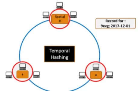
Galileo is a Distributed Hash Table(DHT) based storage system. In Galileo, by convention, each dataset is called a Geospatial File System and can have its own partitioning scheme for the nodes in the cluster. We have selected the modified two-tiered hashing system [29] based on the spatiotemporal characteristics of the incoming data as the partitioning scheme for our datasets. The spatiotemporal observational space of the dataset is partitioned among the Galileo nodes in two phases - the first phase separates the nodes into separate groups, where inside each group, nodes are organized in a ring structure (node-ring) and the second phase puts the groups in another ring called the group-ring. As illustrated in Fig 2.1 the high-level identifier ring is used to partition the data based on the temporal aspect. The time-stamp of incoming data point is used to locate the storage group. Once the group of the storage nodes is identified, the partitioning algorithm will identify the final location (node) to host the data point within the group of nodes. Galileo uses geohash [30] to generate data partitions that store geospatially neighboring data points together. The granularity of size of data block is determined by the length of geohash code managed by the nodes.
Galileo allows users to customize the partitioning scheme based on the type of data acquisition and analytics. The basic unit of partitioning of the temporal domain includes hourly, daily, monthly or yearly. Similarly, the spatial partitioning is fine-tuned based on the geohash precision selected.
Fig 2.1illustrates an example of geospatial data ingestion. As an example, if a client ingests a data point that contains a geo coordinate of (40.5734◦ N, 105.0865◦ W) and temporal information of December 1, 2017, Galileo calculates the hash value of the temporal information using SHA-1 and maps it to a matching group. Then, Galileo calculates the geohash value with the geo-coordinate and determines the node in the group to store the data point (which is 9xvg in this case). Finally, the data is forwarded to the destination node.
Figure (2.1) Node Partitioning Scheme
2.3.2
Galileo Metadata Graph
Each of the Galileo nodes maintains an in-memory data structure called the Metadata Graph. The Metadata Graph is an indexing scheme for local data blocks that speed up data retrieval by avoiding expensive disk I/O. This is especially effective when the system hosts voluminous datasets.
The Metadata Graph is an in-memory prefix tree that holds the metadata information of every data block stored in a node. Every depth-first traversal of this tree represents the metadata of a particular block, with the leaf node holding a path to the block location. For any data access query made to the Galileo system, the Metadata Graph helps reduce the number of target blocks by looking into the metadata information it stores and returning the list of blocks that match the feature constraints of that query.
Fig.2.2 shows a sample representation of the Metadata Graph for a node with three blocks in it each covering the following geospatial domains - {9xvb; 2017-12-01}, {9xvh; 2017-12-01} and {9xvb; 2018-01-01}. Although the figure shows only spatiotemporal features in the graph, it can contain other features from the dataset as well that are queried frequently.
Figure (2.2) Metadata Graph
2.4
Candidate Dataset Properties
Our system is designed to enable integration of heterogeneous spatiotemporal datasets, which are a collection of multivariate records, each containing spatial and temporal information. Our goal is to take two datasets housed in a Galileo cluster and integrate similar pairs of records from the datasets based on their spatial and temporal attributes (we may also add conditions on other features as well).
Our system supports data integration between any combination of data representation models. To examine our system with various types of datasets, we use both point datasets (where each record represents a point on earth0s surface at a particular time) and rasterised datasets (where each record might represent a value for a span in the spatiotemporal domain).
However, the spatiotemporal datasets involved in this operation may contain records of varying resolution. Take, for instance, the US Census data, which is yearly data with records going down to block-group level. So, for a Census dataset, for each result, the temporal resolution is year and
the spatial resolution is a block-group. Compare that to the NOAA Integrated Surface Database (ISD), which consists of global hourly and synoptic observations compiled from numerous sources all over the world. So in this case, the records represent points on the earth0s surface at a particular point of time.
Chapter 3
Relaxed Geospatial Join Across Geospatial Data
Representation Models
In this section, we explain the self-adaptive relaxed spatiotemporal data integration opera-tion in details along with some of the different scenarios, that we may have to deal with, depending on the type of the candidate datasets involved.
3.1
Relaxed Conditions for Data Integration
Figure (3.1) Relaxed Conditions(Geospatial)
Given two indexed datasets A and B, and a spatiotemporal predicate θ (e.g. geospatial area and/or temporal range), traditional spatiotemporal join operation merges the two datasets A and B on the predicate θ. However, the data points, a ∈ A, and b ∈ B, that satisfy the predicate may not have the exact same spatiotemporal attributes. Subsequent analyses often perform data interpola-tion algorithms to generate a virtually integrated dataset that can be ingested to their analysis. This often involves repetitive I/O access and computation.
To provide the estimations as a part of query results, Confluence retrieves spatiotemporally neighboring data points as the query results, in the absence of exactly matching spatiotemporal attributes. Fig.3.1 illustrates an example that estimates an attribute value (from a dataset A) at
the location marked with a red dot. Interpolation algorithms often require neighboring points, marked with black dots (from dataset B) within a pre-defined radius (blue circle). We call the surrounding region retrieved to estimate attribute values at the red point as the relaxation region and the loosened predicate as the relaxed conditions.
Confluence provides a set of spatiotemporal integration operations. The data integration queries support approximate results at the spatiotemporal index of the target dataset. The native data integration operations have the format:
STJoin (target, source, coverage_spatial, coverage_temporal, attributes, relaxation_spatial, relaxation_temporal, model)
This operation imports attributes from the source dataset to match those in the target dataset. To specify a spatial predicate in the query (coverage_spatial) that defines the geospatial query area, users may use a polygon denoted by a set or geospatial coordinates. The temporal predicate of this operation coverage_temporal is specified as a range in the form of two time timestamps or simply time strings. The results will include raw data points match-ing with the coverages, and/ or interpolated estimations. Users can specify interpolation algo-rithms in the query (using (model)) and the Confluence APIs are extensible. The parameters, relaxation_spatialand relaxation_temporal, constitute the query’s relaxation re-gion, which is the spatiotemporal neighborhood for each target record in which we should look for neighboring source records for interpolation. If the interpolation is set as 0, users will retrieve raw data without interpolation. Throughout the rest of the paper, we will refer to the target dataset as F SAand the source dataset as F SB.
Since Confluence supports both vector and raster data representations, this creates four scenar-ios of data integration operation that we might encounter. Table.3.1 depicts the operations over the geo-data representation models.
• Vector-to-Vector: In this operation, both datasets are represented as vector records, similar to the situation in Fig.3.1. In this scenario, Confluence provides a methodology to estimate
Table (3.1) Relaxed Data Integration On Different Datasets Source Data Type Target Data Type Required Data Processing
Vector Vector Overlapping Record Pairs +Interpolated feature Raster Vector Overlapping Record Pairs
+Interpolated feature Vector Raster Overlapping Record Pairs
+Interpolated feature Raster Raster Overlapping Record Pairs
the value of a feature at a point based on the values of the same feature from the relaxation region.
• Raster-to-Vector: This operation imports attributes with an associated raster pixel to be integrated with a group of vector records. The representative raster value is matched to all of the vector points within the raster pixel. In terms of interpolation, Confluence provides an aggregated value of a feature from the vector dataset, representative of the raster pixel, based on the vector points lying in the raster pixel region.
• Vector-to-Raster: In this scenario, Confluence aggregates values of the sources within the area defining a pixel of the rasterized data (target). The interpolation is similar to that of the raster-to-vector case.
• Raster-to-Raster: This operation involves both of rasterized records. The result returns pairs of records from both datasets whose bounds/extent intersect. In this case, due to the lack of an available interpolation strategy that could be applied in a generalized manner, we avoid interpolation.
3.2
Self-Adaptive Relaxation Conditions
If we take a look at Fig.3.1, we can see that the number of neighboring points that get matched against each record of A depends on the size of the blue circle, which represents the spatiotemporal relaxation involved with each data integration operation. We can think of the relaxation region as
a 3-dimensional spherical area (the dimensions being latitude, longitude and time) around each datapoint in A.
Since our integration strategy is based on estimating the value of a point/region based on the observations from neighboring points, each point lying in this sphere will influence the point esti-mate for the value of a feature. In case of most spatiotemporal data, the influence of neighboring points on the value of a feature at a specific spatiotemporal location varies with the region at which we are performing the interpolation. To incorporate this aspect, we introduce a way to dynam-ically tune certain parameters related to the interpolation operation at runtime, depending on the spatiotemporal region we are interpolating at. The dynamic interpolation feature prediction adjusts the influence that the neighboring points have on the final interpolated value of a feature.
In our data integration methodology, we have used machine learning to dynamically influence the interpolation operation by moderating the degree influence neighboring points would have on the estimate. This methodology is explained in detail in section 4.5.
Chapter 4
Methodology
4.1
Distributed Query Relaxation
A simple inner-join operation between datasets A and B would involve only those points from A and B that have a complete match for their spatiotemporal attributes (one-to-one correspon-dence), but, due to the nature of the datasets involved, our relaxed data integration operation yields a one-to-many map as a result. As we can see from Fig.3.1, for a point in dataset A, say Ai, a
collection of k points, say, {Bi0, Bi1, ..., Bik} from dataset B lying in the spatiotemporal
neigh-borhood will be returned as results of the data integration operation, in case an exact match of spatiotemporal attributes is not found.
With such a one-to-many map as the output, we might need to have a one-to-one correspon-dence between F SA and F SB for particular attributes. For instance, in the vector-to-vector
sce-nario, if we have the feature, altitude, in F SA and temperature in F SB. So, corresponding to an
F SArecord with an altitude reading, we will have a set of records in its spatiotemporal
neighbor-hood with different temperature reading. Using our feature interpolation functionality, we aim to estimate the temperature at that altitude with the same spatiotemporal point using the F SB points
that lie in its spatiotemporal neighborhood.
Similarly, in case of a rasterised-to-vector scenario, for a rasterised region for an F SArecord,
we will have multiple vector points from F SBthat are contained in it. Using feature interpolation,
we attempt to estimate the value for an F SB feature for the entire region represented by the raster
record using the set of F SB points in the one-to-many map.
Thus, through our interpolation operation, we want to generate a synthetic value for a feature at the same spatiotemporal location as that of Ai. Also, since the interpolated value is merely
an estimate of the actual value, we also provide an estimate of the uncertainty involved with the prediction.
The methodologies used for interpolation from neighborhood values will be discussed in sec-tion 4.4.
4.2
Relaxation Region
4.2.1
Neighboring Blocks
Since data in Galileo is grouped into separate blocks for discrete geohash and time slice (which could be hour, day of month, month or year), given two blocks B1 and B2 from two separate
filesystems (datasets) whose spatiotemporal domains are not disjoint, either B10s spatiotemporal
range would include B20s spatiotemporal range or vice-versa or B1and B20s spatiotemporal range
could co-incide, depending on what the geohash and temporal precisions have been set for the blocks of those filesystems.
The concept of neighboring blocks comes into play because of the spatiotemporal relaxation condition, since for each block of F SA, the region that needs to be looked at is the spatiotemporal
region covered by the block plus the relaxation region around that block. Neighboring blocks for a particular F SA block refer to the F SB blocks that cover any portion of the relaxation region of
that F SAblock.
As mentioned above, the spatiotemporal bounds of any neighboring F SB blocks will either
fully enclose that of the F SA block, or lie on the edge of the spatiotemporal bound of the F SA
block. Hence, in a case where the F SB block contains the entire bounds of an F SA block along
with its relaxation region, then, a single F SBblock contains both the core data of the F SAregion
along with the relaxation region. In all other scenarios, we might need to scan multiple F SB
blocks.
Having that in mind, if we consider a block of F SA, say BlkAi, and the spatiotemporal range
for BlkAias a cube in the 3-D space (latitude, longitude, timestamp), let0s call it CAi, any block in
F SBwhose spatiotemporal cube externally lies on either of surface of CAi is a neighboring block
To illustrate, let us assume BlkAi is a block of F SA covering the spatial span of 9z and date
29-04-2017, as shown in Fig.4.1. Let us denote a block by the spatiotemporal domain it covers as {9z,29-04-2017}. We can see that spatially, geohashes {c8,cb,f0,9x,dp,9w,9y,dn} are the regions that lie in the immediate spatial neighborhood of 9z. Similarly, the dates 30-04-2017 and 28-04-2017are the immediate temporal neighbors of the temporal region 29-04-2017. So, to summarise, any block covering the spatial region c8, cb, f0, 9x, 9z, dp, 9w, 9y, dn and the temporal range 28-04-2017to 30-04-2017 except for the spatiotemporal region {9z,29-04-2017} is the neighborhood region of the block BlkAi(requesting block).
Figure (4.1) Relaxation Regions
It is to be noted that not the entirety of the data from the neighboring blocks are required for Blki, but rather a bordering spatiotemporal fragment, depending on the relative position of the
block with Blki in the spatiotemporal domain. We call the operation of requesting partial data
from neighboring blocks as Neighbor Data Request.
4.2.2
Maximum Spatial and Temporal Relaxation
This represents the maximum limit to which we can set the spatial (in terms of latitude and longitude) and temporal(in terms of milliseconds) relaxation parameter for a data integration query. This parameter needs to be set before blocks are stored in the filesystem and aids in our new indexing scheme.
It would be extremely time-consuming to fetch the bordering areas of an F SBblock as per the
query relaxations during runtime, since in that case, we would have to go through all the records in an entire block even if we only need a fragment of its data. The maximum relaxations are a way for
the Border Indices to shortlist beforehand the records from a block that fall in the spatiotemporal bordering areas of a block, so that only the shortlisted records get evaluated during runtime.
In our approach, we set the maximum extent of the spatial relaxation that is allowed in a query in terms of geohash characters and the maximum temporal relaxation in terms of milliseconds. In order to make the relaxed data integration operation swift and efficient, there are a few assumptions/ constraints that have to be decided on, regarding the participating datasets (filesystems) during their creation, i.e. before any data blocks are saved. All subsequent data integration queries have to abide by these constraints for the query results to be accurate.
1. Each dataset should specify the values of the maximum relaxation parameters during its creation.
2. In any data integration operation involving two datasets, the query relaxation parameters used must be lower than the lowest maximum spatiotemporal relaxations out of the two datasets.
4.2.3
Maximum Relaxation Region (MRR)
Since the coverage of a block is defined by a geohash, which covers a rectangular spatial plot and a time range, which could be an hour, a day, a month, or a year, we can think of the spatiotemporal extent of each block as a three-dimensional cube. The relaxation region for a block would form an extra layer of coating over this cube. Similarly, a Maximum Relaxation Region is the region formed by coating the original extent of a block with the maximum relaxation parameters for that dataset. So, for a block, Blk, the three-dimensional cube that is formed by combining the original spatiotemporal extent of a block along with its relaxation region is called the Maximum Relaxed Region (MRR) for Blk.
4.2.4
Bordering Region
By bordering regions of a block, we mean any portion of the total spatiotemporal region cov-ered by a block that might be requested as an F SB neighboring block data by another F SAblock
as part of a Neighbour Data Request. As we explain below, the bordering region is defined by the maximum spatial and temporal relaxation parameters that are set for each filesystem (dataset) before actual data blocks are stored for it.
For instance, to extend the example in Fig.4.1, let us assume a block from F SA covering
the region cb, 29-04-2017 (let us call it BlkA) and another block from F SB(BlkB) covering the
spatiotemporal region 9z, 29-04-2017. Now, in case of an integration operation involving BlkA,
the corresponding F SB data from BlkB that is required, is the portion of the block records that
cover the northern flank of the geohash region 9z(as shown in Fig.4.2). No other region from Blkb
is needed for data integration of BlkA.
Figure (4.2) Border Flanks
Hence, we can see that spatially, each block can have 8 possible bordering regions/flanks that may be requested in a neighbor0s data integration- N,S,E,W,NE,NW,SE,SW. The width of each flank depends on the relaxation prameter. Temporally, if the bounds of a block is from time Tstart
to Tend, then the two temporal bordering regions for that block are the regions Tstartto Tstart+ δt
and Tend− δt to Tend. Any combinations of these two sets of flanks are potential bordering regions
for this block that may be requested in another adjacent block0s Neighbour Data Request.
4.2.5
Neighbors
0Orientation
The orientation of a neighboring block with the requesting block determines which fragment of its data needs to be returned as a part of the Neighbour Data Request. The fragments of data being returned as part of a response to a Neighbour Data Request are called flanks.
Let us take the example of the two blocks, {cb, 29-04-2017} (BlkA) and {9z, 29-04-2017}
(BlkB), as mentioned before. The orientation of BlkBwith BlkAis represented as ‘S-Full’,
mean-ing, spatially only the records involving northern flank of BlkBis of interest in a data integration
operation involving BlkAand temporally, all the records are of interest. So an intersection of these
two sets of records, i.e. all records of BlkB that lie in the northern flank are to be returned. In
another example, let BlkA and BlkB be {dn, 29-04-2017} and {9z, 30-04-2017} respectively. In
this case, spatially from BlkBonly data points that lie in the south-eastern flank are of interest and
temporally, only records in the time slice from the beginning of 30-04-2017 to δt milliseconds are to be considered. So the orientation of BlkB with respect to BlkAin this scenario is denoted as
‘’NW-down’(down meaning the temporal range for BlkB lies after that of BlkA).
4.3
Spatiotemporal Border Indexing Scheme
4.3.1
Border Index Overview
Having introduced the various terminology involved, we now introduce our additional in-memory data structure called the Border Index for indexing of the blocks that get staged in the Galileo File System. Similar to the Metadata Graph, this index is created /updated during the stor-age of blocks on a node. However, unlike the Metadata Graph, our new indexing scheme concerns itself with tagging those records in a block that might lie in the spatiotemporal bordering regions. The Border Index is there to help extract the border records from a block, should they be requested as a neighboring F SBdata.
In Galileo, we maintain an in-memory Border Index against each block stored for each file-system (dataset). Each Border Index is tagged to its corresponding block0s absolute path using an in-memory map (called the Border Map) from the path to the Border Index. Each dataset in Galileo maintains its own separate Border Map and a set of Border Indices for its blocks.
The purpose of a Border Index is to tag those regions that lie in the maximum spatial and temporal relaxation regions in a block. It stores the record number of each record that lies in the bordering region of the block along with their orientation. The index is created such that whenever
data from a particular flank of the block is requested (such as ‘S-NW’), we can easily extract record numbers in a block that matches that criteria without having to evaluate the entire block, which could become very time-consuming.
A Border Index is created against each block during its creation. It is then updated every time new records are appended to that particular block. Next, we explain the components of each Border Index to better understand its functionality.
4.3.2
Border Index Components
The Border Index contains in it information about the bounds of different possible spatiotempo-ral flanks along with a list of record index numbers corresponding to each of those flanks. So, one part of the Border Index stores information of the bordering bounds (Flank Descriptors) and the other part keeps track of the record indices that belong to those bounds (Flank Record Indices). It also maintains the total number of records in the block currently.
The Flank Descriptors are information that a Border Index creates during its creation and are never updated after that. These are information that help us determine which spatial and temporal flank to tag a block record to. The Spatial Flank Descriptors in a Border Index contains the list of geohashes that lie on each possible spatial flank for a block. The possible spatial flanks are N, NE, E, SE, S, SW, W and NW (8 in total). Depending on what the maximum spatial relaxation is set in terms of geohash precision, the Spatial Flank Descriptors consists of 4 lists of strings and 4 strings (since the corner flanks are a single geohash), consisting of the geohashes that lie in each of the possible flanks. For example, a block with the spatial coverage of Fig.4.2 in a dataset with maximum spatial relaxation of 3, would have its N, NE, E, SE, S, SW, W and NW flank descriptors as [9xc, 9xf, 9xg, 9xu, 9xv, 9xy], 9xz, [9xx, 9xr], 9xp, [9x1, 9x4, 9x5, 9xh, 9xj, 9xn], 9x0, [9x8, 9x2] and 9xb respectively. The Temporal Flank Descriptors simply contain two pairs(up and down) of numbers that represent the range of timestamp for the upper flank and the lower flank for a block. These descriptors are used to determine which flank a record belongs to and thus tag it to that corresponding Flank Record Index.
The Flank Record Indices contain a total of 10 lists of integers (corresponding to 8 spatial and 2 temporal flanks), where each integer corresponds to the record number from the block that lies in that particular flank. This part of the Border Index gets updated every time there are new incoming records stores in a filesystem block. For spatial Flank Record Indices, if a record lies in any of the spatial flanks, it will get added to its appropriate index list only if it lies in either of the temporal flank (and vice-versa). This means, a record has to lie both in a spatial and temporal border region to make it in either of the Flank Record Indices, since, otherwise, there is need to be checked for check it for a neighbor request.
4.3.3
Figuring out Orientation
Once, based on a neighbor request, we figure out which flanks are needed to be returned, these Flank Record Indices are used to pick out the records that need to be matched against a particular spatiotemporal MRR.
Hence, for instance, if we find that for a block, the flank that is needed to be returned is of orientation ‘E-up’, we just have to find the common indices from the spatial flank indices for ‘E’ and the temporal flank indices for ‘up’ and those are the records to be matched against the MRR bounds.
4.3.4
Neighbor Elimination Using Bordering Index
As mentioned before, for integration for each block, BlkAi, of F SA, we need F SB data for
the region corresponding to its MRR; that amount of F SB data needs to be fed to the thread that
would handle the data integration operation for this particular segment. The data could lie in fully the current node, or a fraction of it could lie in some other node in the cluster from which it would need to be fetched with a Neighbor Data Request.
However, although it is true that, to get accurate results, we need F SBdata from the entire MRR
area, there are spacial cases where certain flanks of the MRR that lie outside the spatiotemporal extent of BlkAiare not needed. Using our indexing scheme, we will show how to further eliminate
certain flanks of the MRR, we will be reducing the spatiotemporal range of Neighborhood Data Request for that particular block which in turn means that 1) the size of data that might need to be transferred from another node (if that portion of F SB data is not resident in the current node) is
reduced and 2) by reducing unnecessary flanks, we also reduce the amount of F SB data involved
in data integration in each thread.
We now explain the specific scenarios where we can reject MRR flanks using the Border Index of an F SA block. For the sake of simplicity, we will be explaining the scenarios in the spatial
domain (2-dimensional) only. The concept could be extended to the spatiotemporal domain (3-dimensional) easily.
Scenario 1: The first scenario is illustrated in Fig.4.3, where the query polygon does not fully contain the geospatial bounds of a block, represented by the brown box. The area between the blue and the brown box represents the geospatial bordering region for the block, which is the maximum spatial relaxation region. As we can see from the figure, the polygon does not pass through the maximum relaxation region of the block on the eastern flank. Under these circumstances, we can see that even after including the spatial relaxation for the query polygon, it would still entirely lie inside the bounds of the block0s geospatial limits on the eastern side.
Hence, spatially, we can ignore querying the geospatial neighbors of the block that would lie to the North-East, East and South-East (as shown in Fig.4.3), since fetching F SBrecords for those
spatial regions would be unnecessary.
Scenario 2: The second scenario is shown in Fig.4.4. Here, although the polygon covers a portion of the eastern maximum relaxation region and it seems like we might need to fetch data for the eastern geospatial flank, we can see that there are no data-points on this block that actually lies in the eastern maximum relaxation region. Hence, in such a case, we do not really need that eastern flank data.
Using the Border Index for the F AAblock, we can easily check if there is data in a particular
flank and then use that information to further optimize the size of the neighboring region that needs to be queried for the block, thus reducing the amount of data to be fetched and possibly the number of neighboring nodes to be queried.
Hence for every F SAblock that matches a data integration query, using the Border Index of
those blocks (like in the two scenarios mentioned above), we can further optimize the size of its corresponding MRR, thus reducing both data movement and record processing time.
Figure (4.4) Neighboring Region Elimination: Scenario 2
4.3.5
Partial Block Processing Using Bordering Index
As mentioned before, by finding the orientation of an F SA block with that of a neighboring
F SBwe can further reduce the amount of data processed out of that F SB block. Since blocks are
defined by the geohash and the time range they cover, it is easy to find it one block from F SB is a
spatiotemporal neighbor of an F SAblock. In case an F SBblock, let us call it BlkBj, is a neighbor
that is in contact with BlkAi0s MRR. That region can be determined by finding out the orientation
of BlkBj with that of BlkAi. The using the Flank Record Indices, we can find the particular record
indices for that particular flank and only those F SB records need to be processed and returned as
candidate F SBrecords for data integration.
Fig.4.5 shows the scenario where an F SB block is a spatial neighbor of an F SA block. We
explain the scenario in the spatial domain only for simplicity. We can see that the F SBblock is the
South-Western(SW) neighbor of the F SAblock. Hence spatially, the only flank that the F SAblock
would need from this particular F SB block would be the North-Eastern flank(NE) and only those
records that lie in the NE Flank Record Indices of the F SBblock should be considered, intersected
with whatever temporal Flank Record Indices are relevant.
Figure (4.5) Partial Neighbor Block Processing
4.4
Feature Interpolation With Uncertainty
The feature interpolation occurs after the record merging operation has completed and is ex-ecuted in the same thread as the segmented data integration operation (explained in 5.1.2). The interpolation strategy we use in our data integration operation depends on the dataset itself and how the data records are influenced by records around them. There is no one specific way to perform spatiotemporal interpolation - the Confluence APIs are extensible to different types of in-terpolation algorithms. Another feature we provide along with an interpolated value is an estimate of the amount of uncertainty associated with that interpolated value. In our work, we explore a few
common interpolation methods that we believed might be effective on the kind of dataset we are working with, which were mostly spatiotemporal sensor or survey datasets.
4.4.1
Vector-to-Vector Interpolation
In the vector-to-vector interpolation scenario, we try to predict the value of an F SBfeature at
a spatiotemporal point for which we do not actually have an observation, but we have a collection of other points in its spatiotemporal neighborhood. In the result of the data integration operation, each point in F SAwill have a one-to-many relationship with a collection of F SB points, since in
most cases the spatiotemporal attributes of an F SAwill not find an exact match with an F SBpoint.
Out of the many available interpolation strategies available, the strategy we adopt is that of the Inverse Distance Weight (IDW) [9]. The reason for picking this strategy is its assumption that the interpolated value would be dependent on observations recorded in its neighborhood, i.e. the value at a certain location is similar to and influenced by the observed values in its neighborhood, which is true for many weather-related or other atmospheric datasets, which are mostly the type of datasets we are dealing with.
In IDW, the goal is to estimate the value of a parameter (Z), at the unmeasured location (Zj)
based on finite set of measurements of this parameter at other locations (Zi), using the following
equation: Zj = n P i=1 Zi (hij)β n P i=1 1 (hij)β
where, hij are the Euclidean distances between the target point and the observed point and β
is the weighting power. As we can see from the equation, the weight or influence of a neighboring point diminishes the further away it is from the location of interpolation. The β determines the rate at which the influence drops with distance. So, the idea here is that the closer a point is, the more influence it has over the estimated value of a parameter.
The optimal β for a particular spatiotemporal interpolation point is calculated using machine learning. We also measure the uncertainty of the interpolated value, Zj, by means of estimating
the error with the machine learning model. This uncertainty value is used to train a model to predict the best beta value and the error rate. The training data for this model is collected using sample data from the dataset and estimating their feature value based on observations from neighboring points and finding the corresponding optimal beta and prediction error.
If the degree of influence of neighboring points is not dependent on the distance, we provide AUEDIN (explained in 6.6.6) as an alternate method for interpolation and error estimation, which involves finding weighted mean of the neighboring data points0feature as an estimate of the feature value and using a weighted standard deviation to estimate the value of the error in the estimate.
4.4.2
Vector-to-Raster/ Raster-to-Vector
The interpolation methodology of the scenario Vector-to-Raster/ Raster-to-Vector is the same, because at the end of the data integration operation, we are left with a one to many map between a raster pixel and a collection of vector datapoints that lie in the extent of the raster area.
So, since each point in the rasterised dataset represents a spatiotemporal extent, we can assume the value of the variable to be uniformly the same in those bounds. Using interpolation in this context, we estimate the value of a parameter from the vector dataset for the entire spatiotemporal extent of the raster record using the vector points that were found as a match. These vector records are treated as observed samples of the variable over the entire raster region and using these sample observational values, our interpolation method predicts a value for the feature over the entire raster extent.
Although several interpolation strategies are available for raster interpolation, we have used one called AUEDIN (explained in 6.6.6). Similar to the vector-to-vector estimation, here also, provide an estimate of the uncertainty involved as a weighted standard deviation among the sample observations.
It is to be noted that in many rasterized datasets, the spatiotemporal bounds/ extent of each record is not explicitly specified. The above method will work only if there is a concrete way to determine whether a point lies within the extent of a rasterised record. For instance, if we consider a Census dataset at county level, just the county name is not enough for us to determine the spatial extent of the records.
4.4.3
Raster-to-Raster Interpolation
A raster-to-raster data integration is possible only if the spatiotemporal extent of the raster pixel of both participating datasets is well defined. This is because, in this case, any intersection in the relaxed spatiotemporal extent of target dataset0s data record with that of the source dataset is considered as a valid integration output and so, there has to be a way to check for intersection. Since intersection of extents is the only criteria for integration here, each record in the output from the target dataset will be mapped to one or more records from the source dataset.
Finding an interpolation strategy in this scenario that can be applied in a general sense is diffi-cult. This is mainly because, in order to interpolate, we have to predict a feature value(from F SB)
that is representative of the entire extent of a record from F SA, based on the F SB records that
intersect with it. To our knowledge, there exists no spatiotemporal interpolation algorithm that can interpolate the value of a raster pixel based on values from area of intersection with other raster pixels. There does exist methodology to interpolate a value for an entire raster pixel based on sam-ple observations from that pixel0s extent, which was the case in case of raster-to-vector scenario, but is not applicable here. Due to this, we avoid interpolation in a raster-to-raster data integration setting.
4.5
Self-Adaptive Relaxation Conditions
The size of the relaxation region determines the records from F SB that are used to determine
the value of a feature at a spatiotemporal point as that of an F SApoint. The size of the relaxation
In Inverse Distance Weighing [9], we have seen that the nearest points have more influence on the interpolated value of a feature at a certain point than those at a further location. Hence, the influence that the points in the relaxation region would have on the interpolated value of a feature decreases with distance. We can think of these neighboring points as sources that have influence over the value of a feature at a given location [31]. The sources in IDW have weights inversely proportional to their distance from the interpolating point. By assigning weights based on the Euclidean distance of the points, we are minimizing the influence that the points further away have on the interpolated value.
The β value in the IDW formula determines the weighing power. It determines by what mag-nitude the influence of a source over the interpolated value decreases with distance. In our im-plementation, we have used a default value of the relaxation region and allowed the value of β to determine how the points further away get penalized. the higher the beta, the stricter the penal-ization with distance. We have thus, in our methodology attempted to find an optimum beta for a fixed relaxation region.
By Dynamic Relaxation Region, we mean that β value of the relaxation region is determined based on the spatial location and the time for the point on which the prediction is being made. Often the level influence of neighboring points on the interpolated value at a point varies with the spatiotemporal region we are trying to interpolate. In order to take that into consideration, we have used machine learning to predict the optimal value of beta based on the spatiotemporal point on which the interpolation is being done. Using a static value of β throughout the spatiotemporal domain of the query would give us inaccurate results from the interpolation operation if there is in fact varying impact of neighboring points based on their spatiotemporal location.
Hence we have implemented a one-time operation to generate training points for our machine learning algorithm and then use them to externally train a machine learning model to predict β, which could then be used during any data integration query to dynamically predict the value of β based on the spatiotemporal region it is dealing with.
4.5.1
Training Data Generation
There is no way to find the optimal β value for each point in F SA during the actual data
integration process since we do not know the actual value of the feature at the point in question. We have, thus, attempted to sample throughout a certain spatiotemporal range and generate a set of training points for our machine learning model. Each training point would have three input features - latitude, longitude, timestamp and one output feature i.e. β.
The training points are generated from a dataset that would be used as F SBin a data integration
query. Out of that dataset, we perform stratified sampling to get N points in total from all its blocks. We then perform data integration between those points in the block on the rest of the points in the block to get a set of neighboring points for each of those N points. For each of the points niin N ,
we use the neighboring points found to predict the value of the feature in question using IDW with different β values. We compare the predictions to find out which β (out of a set of pre-defined β0s) yielded best prediction and generate a training point with the latitude, longitude and timestamp of the point niand β being the target variable. Using these training points, we hope to train a machine
learning model to predict the optimum β.
The Training Data Generation operation is similar to the data integration operation, with the exception that it is an integration of a dataset onto itself and the relaxation parameters involved is the same as the maximum relaxation parameters set for that dataset.
4.5.2
Modelling β Value
We use the training dataset returned to train our machine learning model that takes an input vector of 3 features(latitude, longitude and timestamp) and predicts the value of β. For the pur-pose of supervised learning, we have used feedforward Neural Networks using Python0s SKlearn package.
The optimal model parameters are then printed as a JSON string, to be used as an input in future data integration operation. It is to be noted that for a spatiotemporal region, given the data
distribution is more or less uniform, both the training data generation and the model training is a one-time operation.
4.5.3
Dynamic β Prediction
Our data integration operation supports both using of a static β value or using a trained model to predict optimum β at runtime where, the JSON representation of the trained model is def in as part of the data integration. During runtime, using the trained model0s weights, we make a prediction of beta using each of the F SApoints0spatiotemporal parameters. The F SBpoints in its
relaxation regions are then used to predict the feature value at runtime.
Although it is possible to make a prediction of β value for every F SA point found, it would
be a very time-consuming operation, since the prediction involves multiple matrix multiplication operations, the size of which depends on the layers of the trained neural network. Thus, to simplify the operation, we predict the β for the center-point of the spatiotemporal bounds of every F SA
block involved and use that β for every point in that block. Our experiments show that the error using this method and individual β for every point are quite similar.
Chapter 5
System Architecture
In this section, we explain the various components of data integration operation along with the services that make up the entire Data Integration operation. We also explain the services that go into creating the training data for model building. We will break up the entire operation and explain it in terms of the separate requests that get fired internally once a relaxed data integration operation is requested. Fig.5.2 shows a representation of the various requests and responses involved in a Galileo cluster for a single data integration operation.
5.1
Effective Data Integration
In Galileo, inside each node, the data is partitioned in blocks and each of these blocks is stored in a hierarchical directory structure so that they are grouped by the spatial and temporal character-istics of the data they store.
Typically if records from one dataset(A) are to be merged with that of another dataset(B), based on a set of joining attributes, each record in A needs to be checked against every record in B. This is a O(n2) operation, which is infeasible, considering the size of the data we are dealing with. Even if the data is partitioned into multiple nodes, using this naive strategy on these segments of data on each node is not feasible and would be very time-consuming, as the number of records in a single node is still quite large. This would also require a huge amount of data movement in between the nodes.
So, in order to optimize the operation of data integration in a distributed environment, we mainly attempt to reduce three aspects. First, we need to reduce the network bandwidth utilization by reducing the amount of data transferred in between the nodes. Second, we have to reduce the processing occurring at each node by reducing the number of records being read in for the integration and ensuring that only the records relevant to the integration get processed. Finally, we have to optimize the actual operation of integration of the candidate records from the two datasets.