Mapping HW resource usage towards SW performance

V¨

aster˚

as, Sweden

Thesis for the Degree of Master of Science in Computer Science

-Embedded Systems 15.0 credits

MAPPING HW RESOURCE USAGE

TOWARDS SW PERFORMANCE

Benjamin Suljevi´c

bsc18001@student.mdh.se

Examiner: Moris Behnam

M¨

alardalen University, V¨

aster˚

as, Sweden

Supervisors: Jakob Danielsson

M¨

alardalen University, V¨

aster˚

as, Sweden

Company supervisor: Marcus J¨

agemar,

Ericsson, Stockholm

Abstract

With the software applications increasing in complexity, description of hardware is becoming in-creasingly relevant. To ensure the quality of service for specific applications, it is imperative to have an insight into hardware resources. Cache memory is used for storing data closer to the processor needed for quick access and improves the quality of service of applications. The description of cache memory usually consists of the size of different cache levels, set associativity, or line size. Soft-ware applications would benefit more from a more detailed model of cache memory. In this thesis, we offer a way of describing the behavior of cache memory which benefits software performance. Several performance events are tested, including L1 cache misses, L2 cache misses, and L3 cache misses. With the collected information, we develop performance models of cache memory behavior. Goodness of fit is tested for these models and they are used to predict the behavior of the cache memory during future runs of the same application. Our experiments show that L1 cache misses can be modeled to predict the future runs. L2 cache misses model is less accurate but still usable for predictions, and L3 cache misses model is the least accurate and is not feasible to predict the behavior of the future runs.

Table of Contents

1. Introduction 1

2. Background 2

2.1. Hardware Description Language . . . 2

2.2. Software performance benefits . . . 2

2.3. Cache Memory . . . 2

2.4. Quality of Service . . . 5

2.5. Performance Monitor Unit . . . 5

3. Method 7 3.1. Problem Formulation . . . 7

3.2. Research Questions . . . 7

3.3. Goal . . . 7

4. Curve Fitting Theory 8 5. Implementation 12 5.1. System setup . . . 12 5.1.1 Workload . . . 12 5.1.2 Performance Measurement . . . 12 6. Experiment 14 6.1. Hardware . . . 15 6.2. Evaluation . . . 15 7. Results 17 7.1. Validity of results . . . 17

7.1.1 Improving the validity of the tests . . . 17

7.2. Training set . . . 20

7.3. Summary of R squared values . . . 22

7.4. Evaluation sets . . . 25

7.5. Comparison and summary of results . . . 29

8. Conclusions 33

9. Related Work 34

10.Future Work 36

References 38

Appendix A Graphs of evaluation sets 39

1.

Introduction

Proper mapping of hardware capacity and resource usage is often needed to satisfy demands from user interest down to software performance. Nowadays, system performance is continuously improved and pushed to the maximum due to the development of technology, and it is becoming increasingly difficult to map hardware resources [1]. On the one hand, it is difficult to agree on what the hardware map needs to contain and also which system resources need to be described. On the other hand, it can be challenging to measure and get concrete values for hardware resources. Most of the specifications today are given in the form of data that is not helpful in terms of software performance. For example, when Intel [2] gives information on their processors, they only include the size of their general cache, without any specific details. Recent research [3] [4] focuses on particular parts of resource usage, but to this day, as far as we are aware, no hardware description is focused on software performance. Current process schedulers in CPUs do not consider shared resources when scheduling. This makes it hard to ensure that a specific application of our choosing will have the required quality of service. If we managed to describe the behavior of specific hardware resources, that data could be used to improve the process schedulers and potentially make them shared resource-aware. Having a good model of hardware resource behavior during run-time of an application would go a long way in benefiting software performance.

2.

Background

Description of hardware can be done in a number of ways. The hardware description language needs to be given in the form of a language which both humans and computers can understand. Computers need to understand it to be able to manage the hardware, and humans need to un-derstand it so they can grasp the performance and also the differences between different hardware platforms. Creating such a language can set a standard for describing hardware platforms, or it can be used to describe only a certain group of them. Well-Described hardware can aid and benefit the performance of software since we know the hardware limitations, and therefore can assess the applicability of new software on a system. Multiple hardware resources affect software performance. Such hardware resources are not necessarily integrated into the CPU but can also be provided as peripheral components. Some of the hardware resources include caches, translation lookaside buffers (TLB), floating point unit (FPU), memory management unit (MMU), and others [1]. This thesis focuses on the cache memory, which is described in the following subsections.

2.1.

Hardware Description Language

A way to describe the hardware is using a Hardware Description Language (HDL) [5]. HDL gives a precise, formal description that allows for automated analysis and simulation of the system. HDL is a textual description consisting of expressions, variables, or structures. It can include the behavior of these variables over time as well.

Sometimes it is better to have the description of the system in such a way that we know the execution characteristics of software before run-time. Knowing the execution characteristics beforehand allows the user to gain knowledge on whether a system with a specific hardware platform can run a set of software applications. The virtual validation of system performances requires the modeling and simulation of a complete system.

Nowadays, HDL is dominated by Verilog and VHDL (V stands for VHSIC Very High Speed Integrated Circuits) [6]. These description languages combine design functionality and timing re-quirements while taking into consideration device/platform constraints. VHDL has very extensive and complicated syntax and semantics. VHDL works on three levels of abstraction: on a structural level, on a register transfer level (RTL) and on a behavioral level. The structural level is the actual hardware implementation of a circuit. Behavioral level is the highest level of abstraction and is intended to be easily understood by users. RTL is somewhere in the middle of the two and can be converted in a systematic way to a structural level. Since it covers all of these abstraction levels, it describes hardware vaguely from a software application point of view.

All of the mentioned features have been leading users away from using these languages. Addi-tionally, platform architectures and designs are becoming increasingly more complex by day. This is affecting the code and language provided by these older HDL’s.

2.2.

Software performance benefits

Different kinds of applications stress the hardware resources differently. Optimizing the usage of those hardware resources can be beneficial for improving software performance. Knowing which hardware is compatible with specific software makes it easier to decide on which platform is going to be used to either test or implement the specific application.

This is even more apparent when using multiple software applications on one hardware platform. It is often necessary for more than one software application to use the same hardware resource. Consolidation of multiple functions increases the risk of congestion. If we were to know which application uses which hardware resource and in what quantity, we would be able to schedule an application set more efficiently from a software point of view. Knowing beforehand whether the application set can be executed on a specific hardware saves both time and resources, and can help in picking an optimal hardware platform for that set, instead of being forced to over-provision [1].

2.3.

Cache Memory

Cache memory is used for storing small amounts of data close to the processor for fast access. This fast access is allowed because the cache is typically integrated into the CPU chip. The purpose of

the cache is to store instructions and data that is repeatedly used by the CPU. This type of access increases the overall speed and performance of the system.

Figure 1: Format of the cache hierarchy [7]

Memory Hierarchy

Figure 1 shows the position of cache memory in the system. Multi-level caching has become increasingly used in desktop architectures, where different levels provide different efficiency [8]. The closer a level is to the CPU, the faster access it provides. L1 (primary) cache is the fastest, but also the smallest in terms of data storage. By using this small local cache, we can maximize the execution speed of the applications. The L1 level is usually divided into two caches, one Data cache, also known as the L1D cache and one instruction cache, also known as the L1I cache. L2 (secondary) cache is usually more spacious than the L1 cache and is therefore used to keep larger amounts of data while in exchange we slightly sacrifice speed. L3 cache is specialized to improve the performance of the primary and secondary cache as it is the last level before the main memory. Usage of multi-level caching with multi-core processors usually means that cores can have their own primary and secondary cache, but L3 cache is shared between all the cores.

Performance benefits

The ability of cache memory to improve system performance lies in locality of reference, also known as the principle of locality, which represents the tendency of a processor to access the same set of memory locations repetitively over a short period. Once the locality of reference is known, the information can be kept in the cache memory while safely assuming the system is going to try to access it. Once the cache is full, it needs to free some cache memory in order to be able to receive additional information which is queued into the memory. This is called cache eviction [9]. There are two types of reference locality. Temporal locality refers to the reuse of specific data within a small time duration, and spatial locality refers to the use of data elements within relatively close

Figure 2: Multiple applications using different cores in Multi-core systems [1]

Use in systems

Today’s systems often use cache clusters, meaning that a system can have multiple clusters which all have independent caches (Figure 2. Since real-time systems must be predictable and must meet specified deadlines, hardware resources must be effectively mapped to ensure the deadlines are met. However, cache memories have unpredictable access times, which can result in varying execution times of different runs of the same program [11]. Unpredictable execution times might lead to unexpected behavior of the system, false functionality, or even a deadline miss. This makes cache memories dangerous to use in real-time systems, and therefore, missing the benefits in performance they offer.

Disadvantages of using cache

As the data processing load of the system increases, so does the amount of data/instructions that the processor and cache memory exchange. This way, the cache can become a point of congestion or blockage in the performance of a storage device. Following this, it is necessary to analyze the behavior the cache memory exhibited.

The conflict misses have often been the most significant disadvantage of the cache memory performance and they contribute to the degradation of cache performance. A cache hit refers to a case when the cache memory is accessed and the data/instruction referenced is immediately found and processed. A miss, on the other hand, refers to a case when the referenced data/instruction is not present in the accessed level of cache. In this case, the system suffers from a delay caused by it having to access either a lower level of cache or the main memory (RAM). Cache misses detract from the system performance.

Eliminating conflict misses has remained one of the primary objectives in cache memory ad-vancement. Solutions for lowering the number of misses can address this problem on any number of levels. Many techniques, including alternative cache block placement, were proposed in the past. However, systems nowadays have a more complicated cache hierarchy system which is supporting multiple processor cores. That is why alternative cache block placement is no more producing the optimal number of cache misses. Lowering the number of misses has also been done by eliminating the conflicts occurring under the scenarios where two addresses conflict with each other at multiple levels in cache hierarchy [12]. This method, while not having much to show for in the highest level of cache (L1), shows good results in lowering the number of cache misses in higher levels of cache. This method does not require any additional hardware on the chip.

State of the art improvements

The memory subsystem of modern computers is a complex hierarchy. The cache is now one of the essential components of memory systems, together with registers, physical and virtual memory

on the disk. Recent improvements to cache memory performance were made in regards to hit rate, speed, and energy consumption. Several new designs have emerged, and that for multi-core processors with multi-level caches as well as hybrid caches. Organization of these caches is done via the mapping technique. A mapping technique entails mapping of a larger number of main memory blocks into fewer lines of cache, and set associativity is determined by tag bits within each cache line [8]. Different mapping approaches have different advantages. Replacement algorithm is another crucial element. Cache line replacements can also be done in a number of ways, the most common one being using LRU algorithm (least recently used, which follows a simple logic that the most recently used data is more likely to be used again) [8]. Details of these mentioned implementations are not publicly available. This is another strong argument for requiring description hardware which matches software performance.

2.4.

Quality of Service

Quality of service measures and describes the performance of a service. It can describe a computer network or cloud services, and it usually describes the performance from a users point of view. To measure the quality of service, it takes into account several aspects, like data loss, bit rate, delay, and jitter. Quality of service is essential for the transport of data with special requirements. VoIP (Voice over IP) [13] has been introduced to allow the networks to become as useful as telephone networks for audio. It also supports applications which set strict performance requirements. QoS can be used as a quality measure, as well as referring to applications ability to reserve resources. For example, if we want to measure QoS of a computer application using cache memory, it is exerted with the applications ability to access the cache, the speed of the access and the percentage of cache hits. High quality of service is often confused with a high level of performance, for example, low latency. QoS is also the acceptable effect on a users satisfaction of the application, including all inconveniences affecting the service. It is tightly connected to quality of experience (QoE) [14]. However, QoE is more connected to pleasure or annoyance of users experience with a service and focuses on the entire service experience.

2.5.

Performance Monitor Unit

Most processors today have on-chip hardware used for monitoring architectural events like CPU cycles, cache events (including cache accesses, cache misses, and cache hits), and context switches. PMU helps analyze how an application is performing on the processor. It consists of two compo-nents: performance event select registers, which control what events are to be monitored and how, and event counters, the registers which count the number of events that were chosen by the event select registers. When the event is chosen, the appropriate counter is paired with the event select register [15].

To program the PMU, Model Specific Registers need to be modified. One such 64-bit MSR is given in Figure 3.

Enable Counters bit, when active, enables performance counting in the particular performance monitoring counter. Counter Mask is an 8-bit field which the processor compares to the events count of the detected condition. If the event count is greater than or equal to the value in this mask, the counter is incremented by one [16].

If the PMU is set in Counting mode, the MSRs are configured before run-time. At the end of the monitoring period, the counter values are added and provided as output. In the case of Event-Based Sampling, an event counter is set to overflow after a number of events. This enables the PMU to periodically interrupt the processor and pass the necessary information to the user.

3.

Method

This thesis is formed as an empirical study. Empirical study as a research method fits in this case because data is collected from a performance analysis tool which will include multiple variables whose behavior is observed. After the data is obtained, curve fitting is applied to formulate a model. The results will help understand in which parts of software application run-time the relevant data exerts. This performance model is then analyzed, and it is discussed whether it can predict the behavior of future runs and be helpful and useful from a software performance point of view. What poses the danger here is the validity procedure. Since we don’t have any language to compare the results to, results are valdiated by our own opinion of what is a good result from a software performance point of view.

3.1.

Problem Formulation

Hardware description languages [3] give an overview of hardware features that are not useful in terms of software performance. Mapping hardware resources is a crucial step towards defining and writing a good description language. In this thesis, hardware resource is described, and the description is used to enhance software performance. Using the description could also help evaluate whether a hardware platform and a software application are compatible without having to run the software in question.

This thesis focuses on cache memory, since including all of the hardware resources would make it too broad for a master thesis. The internal memory subsystem of a computer often consists of several layers of cache memories. Data requested by the processor from the main memory needs to be stored in all cache layers before it can be used. If the requested data is already present in the cache, a cache hit has occurred, if not, a cache miss has occurred. Different layers of cache memory can be researched, for example, L1 cache (including L1 instruction cache and L1 data cache), L2 cache and L3 cache. The goal is to model cache memory usage by testing cache misses and use that information toward bettering software performance. The behavior of cache memory is modeled and described using the curve fitting method ??. Curve fitting is a mathematical method of getting a function that fits a given data set and is used for data visualization. The fact that we are analyzing only cache memory as a hardware resource leaves the topic open to potential future work, which can be trying to describe hardware using a different resource.

3.2.

Research Questions

We have formulated the following research questions to address the problems described in Section 3.1.:

• RQ1 - How well can curve fitting be used to model hardware resource usage? • RQ2 - How can the model be used to predict hardware resource usage?

3.3.

Goal

The main goal of this thesis is to describe and model the cache memory behavior so that we can understand and predict the execution behavior in the future. The model will be presented with a curve, which is a result of curve fitting. Testing the model will lead to results which can then be used to predict the behavior in any future runs of the application, which can be on the same hardware platform or a different one. This prediction is to be a step forward in mapping hardware

4.

Curve Fitting Theory

Curve fitting is often used to construct a curve or get a mathematical function that fits a given data set. Depending on the data set, curve fitting can result in an exact fit or a function that approximately fits the data. Fitted curves can be used to visualize data and to infer values where data is missing. There are multiple ways to fit a curve to a data set, including exponential, interpolant, linear, and polynomial [17]. We wanted to have a mathematical way to describe the curve. Cache misses in the system often vary a lot during run-time, and we can expect significant deviations in the measurements, so the polynomial curve fitting is a good way to get a useful description.

Polynomial curve fitting

Polynomial fitting implies fitting a dataset (Figure 4) with a polynomial curve. It is imperative to choose the correct degree of polynomial so that we can get the best fit.

Figure 4: Example of a dataset that needs to be curve fitted [18]

The initial polynomial function is just a line, representing a constant value (Figure 5). The first-degree polynomial is a line with a slope (Figure 6). This line will connect two data points, so the first-degree polynomial is an exact fit of any dataset with two data points with distinct x-axis coordinates.

Figure 6: Dataset fitted with a degree 1 polynomial [18]

The second-degree polynomial results in a hyperbola which is an exact fit for a three-point dataset (Figure 7).

Figure 7: Dataset fitted with a degree 2 polynomial [18]

Increasing the degree of polynomial should, in theory, get us increasingly better fits. As Figures 8, 9 and 10 show, the curve keeps getting better with the higher degree of the polynomial.

Figure 9: Dataset fitted with a degree 10 polynomial [18]

Figure 10: Dataset fitted with a degree 19 polynomial [18]

With this logic, we could find an exact fit for any dataset as long as we find a polynomial of a high enough degree to fit the dataset measurements. This, however, is not true. Runge’s phenomenon [19] is a problem of polynomial interpolation non-convergence. It occurs when using polynomials of a high degree to interpolate between two data points. This phenomenon was the first one to show that using higher degrees of polynomial does not always improve accuracy. From Weierstrass theorem [20] we expect that using more points would lead to a more accurate reconstruction of the function. However, polynomial functions are not guaranteed to converge uniformly. The theorem states that one set of functions exists which meets the conditions of uniform convergence, but it does not provide ways to find it. Not only does increasing the polynomial degree not necessarily improve the fit of the curve, but it can also lead to overfitting [21].

Underfitting

As much as overfitting is a problem, underfitting is not any better. A model that is under fitted is less flexible and can not account for all the data. Underfitted models usually have low variance and high bias. These models disregard a lot of the data and instead make assumptions about it. The bigger the underfit, the stronger assumptions are made. The data these models are ignoring is usually important replicable data, and without it, the model fails to identify the effects that the data supports. The mistake of underfitting can be improved with increasing the polynomial degree to get a better fit for the data, and with that, a better model.

Overfitting

Overfitting is generally using a more complicated approach than necessary. In our case, it refers to the case of using models that include more terms than necessary. There are two types of overfitting: overfitting with a model that is more flexible than needed and overfitting with a model that has irrelevant components. Using a polynomial of a higher degree than necessary means that the used polynomial includes excessive components, and usually means that a polynomial of a lower degree could be a better fit for the dataset. Another danger lies in some random excessive polynomial degrees resulting in good fits [22]. For example, we fit a dataset with a polynomial curve of fourth

degree with a fit of 80%. We continue increasing the degree, but we get worse fits of 40%. Then with the seventh-degree polynomial, we get a 70% fit. This instability is upsetting because the close match these two degrees have. This can be noticed if we test enough degrees, but in most cases it is enough to start noticing the decent of the fit the curve has.

Overfitting is not only unnecessary but also undesirable in many cases. Aside from getting worse fits, adding polynomial degrees that perform no useful function means that using this polynomial in the future will always calculate the excessive degrees and record them. Increasing the size of the polynomial also questions its portability. A lower degree polynomial is easier to apply by anyone else in the goal of duplicating or testing results.

5.

Implementation

Firstly the software application is chosen. Secondly, since the idea is to describe cache memory usage, a proper way to measure cache memory characteristics is picked. Finally, a suitable way of analyzing the collected data is needed.

In the following subsections, we describe:

• Workload - which is a matrix multiplication - 5.1.1 • Tool for measuring the performance counters - 5.1.2

5.1.

System setup

In the following subsections, we describe the workload used in test as well as a way of measuring and collecting the performance data. Tests are run on Linux 4.18.0-20-generic. The code is written in C, and the gcc 7.3.0 compiler is used. As for the workload, matrix multiplication was chosen as an appropriate software application. Performance Monitor Unit was used to measure the performance and collect data.

5.1.1 Workload

Matrix multiplication is a binary operation that produces a matrix as a result of a product of two matrices. This product is designed to represent the composition of linear maps represented by matrices, therefore making matrix multiplication a basic tool of linear algebra. Its frequent usage is in linear maps, systems of linear equations and dot products (bilinear forms). It has a simple implementation of the basic (often called naive) algorithm, with the possibility to expand it and make it more complex. Even though matrix multiplication can be a product of any two compatible matrices, from here on out when it is said matrix multiplication, we imply a product of two square matrices. The naive implementation gives it a complexity of O(n3) [23]. However, this is not optimal, as the complexity was lowered over the years with the modifications of the algorithm. Up to date, the lowest complexity reached is O(n2.3728639_{) [23].}

The reason why the matrix multiplication is important in the computational complexity is that many algorithmic problems have the same complexity as the matrix multiplication, or have a complexity that can be expressed with the complexity of matrix multiplication [24]. Also, many of the algorithmic problems can be solved using matrix computation.

If the matrix multiplication is part of a bigger application, it can be harder to pinpoint the influence each part had on the time complexity and the cache memory, so we decided to do the tests on the implementation of matrix multiplication. The size of the matrix plays a role in the execution time as well. On the one hand, if a large matrix is used, the execution might take longer to execute. On the other hand, if the matrix is too small, the number of samples will be too low. We decided on a 1024x1024 matrix. We have three arrays with each array being 4 bytes, so 4bx1024x1024 = 4M B. In total comes up to 12MB, which is, for example, four times the size of the L3 cache on the used platform.

5.1.2 Performance Measurement

Hardware resources can be measured by using software tools. These tools use the Performance Monitoring Unit (PMU) to collect data on different hardware resources. The PMU uses a set of special purpose registers called hardware counters to store the data of hardware events. PMU helps conduct low-level performance analysis. The most popular performance analyzing tool for Linux is perf [25]. Perf is capable of statistical profiling of the system, including the kernel and user-land code. Other tools include OProfile [26] and Performance Application Programming Interface (PAPI) [15].

Performance Application Programming Interface

PAPI provides an interface for the use of the hardware performance counters found in most mi-croprocessors. That interface consists of a simple, high-level interface for simple measurements

and a low-level programmable interface for more sophisticated needs. Using the low-level interface allows access to data such as relating cycles to memory references or cache memory misses. It also provides options for controlling the counters, setting the thresholds for interrupts and access to all native counting modes and events. By multiplexing the counter hardware, PAPI can count a larger number of events simultaneously. Multiplexing unavoidably introduces overhead which can affect the accuracy of counter values, but depending on the use of the data, this overhead can be disregarded [27].

An important part of the methodology was choosing which cache memory features are going to be measured and analyzed. Some interesting counters available in PAPI include cache hits and misses for all levels of cache (data and instruction caches), requests for access to cache line, cache accesses and reads, instructions issued and completed, lookaside buffer misses and cycles stalled. Cache misses carry much weight in general cache memory performance. The reasons for cache misses can be: the information that the application wants to store in the cache memory is larger than the available cache memory at that moment, the information that the application wants to store can not fit in one piece (on one address) and needs to be partitioned or the data on the address is being used by more than one thread. Data on when an application has a higher number of cache misses can help to know at what time during the execution the application requires more cache memory access than usually and also gives information on whether the application needs the information in the cache memory needs to be protected. In the analysis of the cache misses during the whole run-time of the application, we can notice when the application has a higher demand of cache memory and potentially inform the scheduler to clear the cache during that time. Knowing this would allow the application to run more smoothly.

6.

Experiment

The tests consisted of running an instance of a 1024x1024 matrix multiplication a certain number of times (this number is discussed later on in this section). As mentioned in section 7.1., the core affinity is set for the process, so the application was running on one core the whole time. This ensures the application will access the same parts in the cache memory, so no additional cache misses happen on accident. Since the goal is to predict the behavior of cache during the execution of the application, a training set is made for that purpose.

The test procedure is illustrated in Figure 11.

Figure 11: Test procedure

The test procedure shown in Figure 11 represents the procedure for getting the training sets. Depending on the chosen performance event, different data is measured during each iteration of matrix multiplication. The performance events being measured for training sets are L1 cache misses, L2 cache misses, and L3 cache misses. Firstly we initiate the matrix multiplication by generating the matrices. The matrices are generated with a fixed size, and their elements are random. Secondly, the loop is started. The number of iterations is preset. During the iterations, performance is measured depending on the selected performance event. Data on performance is available for every iteration. When the required number is reached, iterations are stopped, and the mean value of the chosen performance event is calculated. The mean values of all the iterations

represent the mean value for the instance and the training set.

It is important to highlight that each test is run ten iterations before starting the measurement to ensure the cache is warmed up. For example, if the instance is tested with five iterations, that means the instance is run with fifteen iterations, where the first ten are warming the cache up, and the remaining five are the ones we are taking into consideration.

The number of iterations per instance is a crucial question in making a good and reliable training set. Firstly the test was run with five iterations in one instance. After finding a mean value of the instance by using the specified number of iterations, the initial test was checked against another one with also five iterations. Analyzing these results, we considered increasing the number of iterations to get more credible results. Figure 12 shows how the number of iterations in one instance affects the mean value of the instance. X-axis represents number of samples, and the Y-axis represents total number of L1 cache misses.

Figure 12: Different number of iterations per instance

The blue line, representing five iterations, is very similar to the red one, which represents 15 iterations per instance with some higher peaks. The line representing 100 iterations differentiates from the other ones on a few parts, so we can assume it is going to give more information in the long run.

6.1.

Hardware

The environment is an Asus laptop with dual-booting Linux operating system with Windows 10. The hardware specifications are given in table 1.

Table 1: Hardware specifications Asus Vivobook S14

Feature Hardware Component

Core Intel(R) Core(TM) i3-6006U CPU @ 2.00GHz L1 cache 32KB 8-way set assoc cache/core

error, R squared, and modified R squared [28]. R squared method can be applied to any dataset and is usually the method used for evaluating the goodness of fit.

R squared method

R-squared [29] measures how successful the fit is in explaining the variation of data. It is defined as the ratio of the sum of squares of the regression and the total sum of squares.

Rsquare = SSR SST = Pn i=1wi(ˆyi− ¯y) 2 Pn i=1wi(yi− ¯y)2

R squared is defined as quotient of sum of squares of the regression and the total sum of squares. wi represents a weight coefficient which can be included or not included in the calculation. ˆyi is

the estimated value of the output, ¯y is the mean value of the output while yirepresents the output

value itself.

R squared can take any value between 0 and 1, representing the percentage of how much does the curve fit the dataset. However, depending on the dataset, a low R squared value is not always bad, and a high R squared value is not always good [30]. It is possible that a high R square value is achieved, but the results are biased. Furthermore, if the R squared value is low, it is still possible to draw meaningful conclusions based on the shape of the curve. The significant coefficients can still reflect the change in the values, and we can still draw meaningful conclusions about the relationship between the variables. This type of information is still valuable.

7.

Results

In the following sections, the results from the experiments are presented. First validity is addressed, and what was done to improve it. Secondly, the results of the test are presented, including training sets and evaluation sets. A specific section addresses the R squared value of applying different polynomial degrees to fit the training sets. In the end, a conclusion is given, where research questions are debated.

7.1.

Validity of results

The construct validity investigates the relationship between theory and observations made, specif-ically whether a test measures the intended construct. Having access to Performance API (PAPI) [15] allowed us to choose the performance event we want to measure, including cache misses for all cache levels. Tests show that the implementation fulfills the planned and desired functionality, which was collecting and measuring the performance data on a specific hardware resource, cache misses in particular.

Since initial tests had a big difference in execution times, the initialization of the matrix was moved to be before the start of the iterations. This makes the test more restricted and endangers generalization possibilities, but without this, we would be analyzing iterations with different exe-cution times, which could lead to wrong conclusions being drawn from the data analysis. External validity cannot be guaranteed since only the behavior of this particular working set was described, and the experiment did not include more than one platform in testing. However, internal validity represents how well an experiment is done. In other words, if a study is confusing, the internal validity is low. Also, it is important to rule out alternative explanations for the findings. This is addressed in the section below 7.1.1.

Conclusion validity describes if the right conclusions were drawn from the available data. To support conclusion validity, the number of iterations in the training set is increased (section 6.). Additional support would have been choosing a better performing hardware platform and testing on multiple different platforms. There is no guarantee that the results will be valid on other platforms.

7.1.1 Improving the validity of the tests

The initial tests are run without any preparation. A script running an instance of matrix multi-plication and measuring the cache misses is used. Three different events are measured using the Performance API, including L1 cache misses, L2 cache misses, and L3 cache misses. The script was called using the terminal in Linux. The first thing that is noticed is that some iterations within this instance finish earlier than the rest. To be able to plot and analyze the data, the shorter instances were extrapolated with the ending value until the other runs ended. After some analysis, we realized that the matrix multiplication was generating random elements inside the matrix at the start of every iteration. This has caused some runs to last way longer than expected, and some runs finished earlier. This problem was present in all of the cache levels and it had a random effect on them, so there was no noticeable pattern.

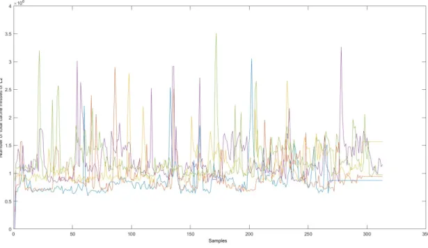
Figure 13: Number of total cache misses in L1 (different colors represent different iterations) Looking at the L1 cache (Figure 13), see that some iterations have very different behavior. For example, while the green line becomes relatively stable after 170 samples, the other ones still have very non-deterministic behavior. While the blue line has an average value of around 5x106_{, the}

red line has a much lower average, 3x106. Also, from this instance of matrix multiplication, we can not say that any of these iterations have any behavior in common. All of them look very unstable and not usable.

Regarding the L2 cache (Figure 14), the situation with the average values is better than in L1. All of the iterations average around 1x106_{. These sudden spikes represent the weird behavior}

in this level of cache, and they are not natural. We tried to notice some pattern and discern a possible periodical behavior. For example, the green line has two spikes in the beginning (samples 20 and 30) and then two spikes later (samples 170 and 200). The blue line has three big spikes with approximately the same distance between them (samples 60, 130, and 200). However, even if these represented some periodical behavior, it would still not be useful since iterations inside the same instance have different behaviors and different periods.

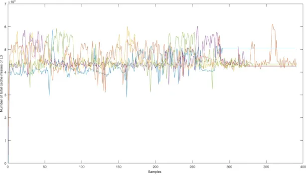
Figure 15: Number of total cache misses in L3 (different colors represent different iterations) The behavior of L3 cache (Figure 15) might be the best one out of the three, but it is still not useful and challenging to analyze. The average value of the iterations is around 4.5x105, but the individual iterations still have very non-deterministic behavior. Some iterations might exert similar behavior in certain parts of the run, but in the other parts it is entirely different. The spikes that are present are positive for some iterations, and for others the spikes are positive. This renders the information almost useless and impossible to analyze further.

To remove the problem with variable execution times, we fixed the code so that all iterations inside one instance do matrix multiplication with the matrix of the same size and containing the same elements. This will, later on, prove to be a good solution, since it fixed this problem and made all iterations have the same number of samples taken. It also introduced a threat to validity, which is addressed in 7.1.. It is safe to assume that this also helped the problem of not having a stable average value for iterations inside one instance. Core affinity is set so that all the iterations happened on one core. After analyzing the spikes, we figured out that they probably originate

this, it could be ensured that no other programs could interfere with the execution of the matrix multiplication application by making a separate partition only for that application. However, using control groups seemed too strict because we are trying to set the conditions as they would be from another users perspective. If a user were to run an instance of matrix multiplication to check whether the prediction is right, they would run the application in a natural environment. The information we are going to provide this way is going to be more helpful than if control groups were used to make the process more strict.

7.2.

Training set

Since the procedure is straight, the test can be run. The training sets for L1 cache, L2 cache, and L3 cache are shown in Figures 16, 17 and 18.

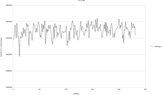
Figure 16: Training set for L1 cache showing the mean value of L1 total cache misses over 100 iterations

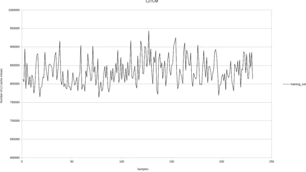
Figure 17: Training set for L2 cache showing the mean value of L2 total cache misses over 100 iterations

hard to model. Similar conclusions go for L2 cache misses and L3 cache misses. L2 total cache misses training set in Figure 17 starts as good as the L1 cache misses, but in the middle it looks like the signal increases its frequency. L3 total cache misses training set is the worst of the three since it has the fastest changes. It is safe to assume that because L3 is the biggest cache memory in the system, so most of the other applications use it.

7.3.

Summary of R squared values

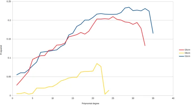
It is crucial to choose the right polynomial degree to get the best fit possible. We tested the goodness of fit for different polynomial degrees until the R squared value started stagnating. Figure 19 plots the goodness of fit in function of polynomial degree for all cache levels.

Figure 19: R squared value in function of degree of polynomial for all cache levels

Figure 19 shows a clear indication that the 29th degree of polynomial is the best fit for the L1 cache misses training set with the goodness of fit of 23.45%. The 25th degree of polynomial is the best fit for the L2 cache misses training set with the goodness of fit of 20.9%, and the 21st degree of polynomial is the best fit for the L3 cache misses training set with the goodness of fit of 8.5%.

As expected from the behavior exerted by the data sets, L1 cache misses training set gives the best model out of the three. The L2 cache misses training set model gave slightly worse goodness of fit than the L1 cache training set. However, we are still able to determine time intervals during the execution time in which the application provides a higher number of cache misses. The L3 cache misses training set provided the worst goodness of fit of the three.

The models shown in Figures 20, 21 and 22 can be used to evaluate in which parts of the applications execution time are we having more cache misses than the rest. There are clear parts which show the increase in the value of cache misses, which means the application is requesting more cache access at those times or something is blocking the applications access and interfering with data in reserved cache memory. This information can be used by the scheduler to determine times when the application needs more cache memory or the cache memory it is using needs to be protected to ensure the software performance of the application.

R squared values

Polynomial degree L1 training set L2 training set L3 training set 1 0.054907106912482 0.027144168587126 0.004954475 2 0.060331027844363 0.039049729289024 0.005153299 3 0.060339928729903 0.051787389687552 0.007732529 4 0.068573189265968 0.064169309672833 0.003676192 5 0.079261686045211 0.096030226761342 0.005650769 6 0.088978438553909 0.101236133069984 0.019607171 7 0.114792133012818 0.105828642451022 0.01966105 8 0.116359392571394 0.106135462025395 0.019849945 9 0.117723411038289 0.119960569902474 0.02305845 10 0.119703348283486 0.121488736076412 0.023865777 11 0.121276104144986 0.134011616005271 0.030081854 12 0.130156174505271 0.134800914913514 0.038514975 13 0.135843451778331 0.13903779145196 0.042041912 14 0.160921326604266 0.156018241663548 0.046570216 15 0.165716394898554 0.158704301937069 0.048459029 16 0.183746208189594 0.16186733027008 0.048498066 17 0.189570763078486 0.167638949572364 0.062337574 18 0.200363818621901 0.163258002193029 0.064010247 19 0.200434201939207 0.170943090343049 0.064152219 20 0.207381090011834 0.18758589395364 0.064990132 21 0.216426582021646 0.203312839750325 0.085037769 22 0.217720107537946 0.203272886939118 0.077353248 23 0.216227639188773 0.204247830813567 0.003552586 24 0.215679118786092 0.203130498872962 0.014051558 25 0.215559151229952 0.209739558102903 26 0.216074190107605 0.202488824986858 27 0.220411433499101 0.200562656672509 28 0.232648109607558 0.195529436776323 29 0.234575274157325 0.194351091802704 30 0.225668746308703 0.189161258272597 31 0.227033094624053 0.194055732648867 32 0.225094298519529 0.178573829218008 33 0.231170735212568 0.132079291961024 34 0.224420676747148 35 0.164963075379825

Table 2: R squared values of training sets

Table 2 gives the R squared values for all polynomial degrees for all levels of cache. From these results, it is clear which polynomial degrees give the best fit for the curve. Applying the best polynomial degrees to corresponding training sets resulted in curves shown in Figures 20, 21, and 22.

Figure 20: Training set for L1 cache showing the mean value of L1 total cache misses over 100 iterations with a fitted curve using 29th polynomial degree

Figure 21: Training set for L2 cache showing the mean value of L2 total cache misses over 100 iterations with a fitted curve using 25th polynomial degree

Figure 22: Training set for L3 cache showing the mean value of L3 total cache misses over 100 iterations with a fitted curve using 21th polynomial degree

7.4.

Evaluation sets

After the training sets are fitted with curves with the best goodness of fit, a few more instances of matrix multiplication are tested, and it is checked if the resulting model can predict the behavior in the future runs of the application. These instances are called evaluation sets because they are used to evaluate the ability of the training set to predict the behavior of cache memory misses. Five more instances of matrix multiplication are run, each one with five iterations. Graphs shown in Figures from 23 to 28 represent the mean value of each of the instances, making evaluation sets.

Figure 23: Third evaluation set of L1 cache misses

Figure 25: First evaluation set of L2 cache misses

Figure 27: Second evaluation set of L3 cache misses

Figure 28: Fifth evaluation set of L3 cache misses

Looking at these mean values, we can see that not all evaluation sets of one level of cache have the same mean value. For example, fourth and fifth evaluation sets of L1 cache misses have a mean value around 5.5x106, while the rest of the evaluation sets for L1 cache misses average at or below 5.4x106_{. Regarding the L2 cache misses, mean values of evaluation sets oscillate between 8x10}5

and 10.5x105_{. The L3 cache misses of the evaluation sets are mostly at 2.5x10}5 _{(third, fourth}

and fifth evaluation set), while first and the second set are a little higher, 2.6x105 _{and 2.7x10}5_,

7.5.

Comparison and summary of results

Since the training sets and five evaluation sets are complete, we can proceed to comparison between the two. The comparisons are given from Figure 29 to 34.

increases of cache misses in all five evaluation sets except the one in Figure 30 around sample 80. The prediction of the cache misses is not always of the same intensity, but their existence was predicted and confirmed.

Figure 31: Comparison of curves of training set and the second evaluation set of L2 cache misses

Figure 32: Comparison of curves of training set and the fourth evaluation set of L2 cache misses As for L2 cache misses, four out of five evaluation sets have behavior which mainly sticks with the average value without having many variations. This is why a lot of the predicted behavior by the training set did not happen in the evaluation sets. The noticeable changes in behavior in the evaluation sets were predicted by the training set correctly, as shown in the Figures 31 and 49. The evaluation set in the Figure 32 has a behavior that is different from the other ones and has

weird and inexplicable spikes in the number of cache misses that have not been shown by either the training set nor the other evaluation sets. The evaluation set that showed the best results regarding predicting its behavior is in Figure 31.

deviations, behavior which was matched only by one evaluation set in Figure 33. In Figures 34 and 53 the model predicts some behavior at the start and near the end of execution, but mostly the behaviors of curves do not match.

When summarizing these results, it is important to notice that the polynomial degrees chosen for the training sets are not necessarily the best fitting ones for the evaluation sets as well. For example, when one of the evaluation sets curves polynomial degree was changed, we got a better fit for that evaluation set (Figure 35. In this thesis, we show results only plotting curves with the polynomial degree that showed the best fit for the training set. This is because the training set is used to predict the behavior of the future runs so the same polynomial degree should be predicted.

Figure 35: Comparison of curves of training set and the fifth evaluation set of L1 cache misses (adjusted polynomial degree)

8.

Conclusions

Our goal was to make a model for cache memory and use that model to predict behavior in future runs. RQ1 was about modeling the hardware resource and checking how well does that model represent the behavior of the resource. With these results, we answered our first research question. Even though these models do not give high goodness of fit, that is because the data is scattered in that way, and we can still use the model to draw important conclusions on the behavior of the cache memory during run-time of the application. This model is the first step towards developing a hardware description language which benefits software performance.

The RQ2 was about using the model from RQ1 to predict the behavior of the hardware resource in the future. After analyzing the results, the L1 cache misses model was able to predict the deviations in behavior of the evaluation sets. This is very valuable and can be potentially used by the scheduler to predict when an application is going to have a higher demand of the L1 cache access or when an application is in danger of having a higher number of cache misses than usual. The L2 cache misses model was able to predict the most prominent deviations in behavior of the evaluation sets, but it had a problem of predicting things that did not happen and this has made the model worse. The L3 cache misses model was not able to predict behavior of the evaluation sets. The training set was not predicting almost any deviations from the average value, while the evaluation sets did not fit that at all.

9.

Related Work

Even though software performance modeling is a broad area and has been researched before, this particular take on modeling has not been researched a lot. Therefore there are not many papers re-garding it. Research in this field includes using different software performance tools [27] to measure the behavior of a software application during run-time [31], multi-core performance measurement [15] and some software performance anti-patterns [32]. However, software performance has not yet been measured toward checking the hardware resource usage.

The first paper chosen researches hardware resource aware scheduling [1].

Increasingly more telecommunication fields introduce multi-core platforms to their systems. It is important to separate processes which are cache bound by the same level of cache, as to not overload a core. It is suggested to divide the applications using the same level of cache among more cores to increase the system performance. Of course, the optimal process allocation is not always possible. The paper thought of a process scheduling method that ensures the efficiency of QoS for processes that run on a shared hardware platform. The OS allocates processes depending on the system load, CPU usage of individual processes and settings for power consumption. However, there is a privileged accessible affinity functionality, which allows the designer to determine what CPU core the process should use statically. Using this feature, we can develop a new scheduling method by determining which process is going to use which core before run-time. This would mean that if a process has a set core affinity, its performance should not be affected by a process that has an affinity to a different core. To do this correctly, we need the information on the usage of hardware resources by different applications. Performance Monitor Unit (PMU) [16] is used for monitoring resource usage. Our thesis has a different goal, hence, the different approach. We are running one application on one core and trying to minimize the effects of the other processes. There is no point in making sure that our process has the optimal process allocation since we do not have any other processes which explicitly try to endanger the QoS of our process. The processes which might interrupt and interfere with ours are the processes that we can hardly impact or control. The other option would be to shut them off completely, but that was addressed in section 7.1.. We do not have to worry about making sure that our process has the optimal process allocation. We are trying to use the data from the tests to model the behavior of the cache memory during run-time of an application. This model might help towards developing a new scheduling method which uses the model to predict the behavior of future runs of the application and determine which processes will use which core at what time accordingly. Also, our model might benefit a scheduler which dynamically changes the cores, considering the predicted behavior of the software applications.

The second paper researches a new scheduling architecture towards enforcing the quality of service [33].

The scheduling method determines a process for which we want to enforce QoS and then mon-itors the hardware resource usage during the run-time of the said process. The data on hardware resource usage, together with process performance, is used to ensure that enough resources are provided for the chosen process. To make sure of that, we might deny access to resources to other processes until we are sure that our process has used the resources allocated to it. This can bring into question the danger of neglecting specific processes or giving the chosen process advantage over an internally more critical process. To counter this, there is a possibility to set constraints and get fair scheduling of resources. A method to schedule processes according to their resource usage was devised. Additionally, a mechanism was used to generate an interrupt whenever a resource quota is reached, meaning the shared resource usage of the chosen process minimizes the effect on other processes and the shared resource usage of all other processes in the system does not affect the resource usage of the chosen process. This ultimately ensures the general performance of the chosen process. This work explored the option of assigning different processes to different cores to benefit the performance of the process. If this is done correctly, it can hugely benefit the software performance. The paper contributes by developing an architecture to help schedule processes ex-ecuting on a shared hardware resource. If the scheduler is not aware of the shared resources, it might affect the applications WCET. As mentioned above, the cache misses affect the execution time of a task, and they introduce the non-deterministic element. If the shared cache memory is not ”protected” in a way that the scheduler is aware of whoever is using at any moment, that can endanger the application or even the system it is running on. This concern intensifies in high-level

systems where the danger lies in both the data and the instruction cache. A common goal of our thesis and this paper is to enable a scheduler to be resource aware and use that to improve software performance. During our testing, we also tried to make sure that enough hardware resources were given to the observed process (7.1.1). Instead of analyzing the measured data during run-time, we intend to measure the data and use it to model the behavior of cache misses throughout different levels. In our approach, the model is used as a predicting tool. This would exclude the usage of measuring tools (PAPI [15] during every run-time, but would instead use the generated model to predict when specific processes should be scheduled. This would remove the aspect of real-time measuring and comparing resource usage and process performance. However, using a model in-stead of having to gather data during the execution of the application would considerably lighten the load on the processor and would enforce quality of service by itself.

10.

Future Work

Since modeling of cache memory and using it to predict the future behavior was not, as far as we know, researched before, we are hoping to incite others to try and research this field more. Software performance can benefit from this field, mainly because it is tightly connected to several other fields, like QoS, execution time analysis of applications, and general cache memory research. As future work, we would suggest building upon the work done in this thesis. This includes testing with a different number of iterations and changing the polynomial degrees dynamically during testing. It would be interesting to check the best goodness of fit for each of the evaluation sets to check if that would help the model predict the behavior better. The goodness of fit can be evaluated using different evaluation method. It would be good if these tests could be run on different hardware platforms or multi-core hardware. These test can also be executed while measuring and keeping track of different events than cache misses. It can also be researched what events can be modeled better than others, and which ones can predict future behavior the best.

Since these test instances were run with matrix multiplication, we can consider running tests on multiple different software applications to see which ones can be modeled better and to identify the challenges we meet modeling the cache memory. In the end, one can also try to measure and describe other hardware resources to try and contribute to software performance.

References

[1] M. Jagemar, A. Ermedahl, S. Eldh, M. Behnam, and B. Lisper, “Enforcing quality of service through hardware resource aware process scheduling,” in 2018 IEEE 23rd International Con-ference on Emerging Technologies and Factory Automation (ETFA), vol. 1. IEEE, 2018, pp. 329–336.

[2] I. Corporation. Intel core i3-330m processor. [Online]. Available: https://ark.intel.com/ content/www/us/en/ark/products/47663/intel-core-i3-330m-processor-3m-cache-2-13-ghz. html

[3] A. Burlakov and A. Khmelnov, “The computer architecture and hardware description lan-guage,” in Information and Communication Technology, Electronics and Microelectronics (MIPRO), 2015 38th International Convention on. IEEE, 2015, pp. 1066–1070.

[4] O. Port and Y. Etsion, “Dfiant: A dataflow hardware description language,” in Field Pro-grammable Logic and Applications (FPL), 2017 27th International Conference on. IEEE, 2017, pp. 1–4.

[5] Y. Li and M. Leeser, “Hml: an innovative hardware description language and its translation to vhdl,” in Design Automation Conference, 1995. Proceedings of the ASP-DAC’95/CHDL’95/VLSI’95., IFIP International Conference on Hardware Description Lan-guages. IFIP International Conference on Very Large Scal. IEEE, 1995, pp. 691–696. [6] E. Christen and K. Bakalar, “Vhdl-ams-a hardware description language for analog and

mixed-signal applications,” IEEE Transactions on Circuits and Systems II: Analog and Digital Signal Processing, vol. 46, no. 10, pp. 1263–1272, 1999.

[7] M. Rouse. (2014) what is cache memory? - definition from whatis.com.. [Online]. Available:

http://searchstorage.techtarget.com/definition/cache-memory

[8] M. T. Banday and M. Khan, “A study of recent advances in cache memories,” in Contemporary Computing and Informatics (IC3I), 2014 International Conference on. IEEE, 2014, pp. 398– 403.

[9] W. Stallings, Computer organization and architecture: designing for performance. Pearson Education India, 2003.

[10] C. Xu, X. Chen, R. P. Dick, and Z. M. Mao, “Cache contention and application performance prediction for multi-core systems,” in Performance Analysis of Systems & Software (ISPASS), 2010 IEEE International Symposium on. IEEE, 2010, pp. 76–86.

[11] M. Milligan and H. Cragon, “The use of cache memory in real-time systems,” Control Engi-neering Practice, vol. 4, no. 10, pp. 1435–1442, 1996.

[12] H. Salwan, “Eliminating conflicts in a multilevel cache using xor-based placement techniques,” in High Performance Computing and Communications & 2013 IEEE International Confer-ence on Embedded and Ubiquitous Computing (HPCC EUC), 2013 IEEE 10th International Conference on. IEEE, 2013, pp. 198–203.

[13] B. Goode, “Voice over internet protocol (voip),” Proceedings of the IEEE, vol. 90, no. 9, pp. 1495–1517, 2002.

[17] H. Akima, “A new method of interpolation and smooth curve fitting based on local proce-dures,” Journal of the ACM (JACM), vol. 17, no. 4, pp. 589–602, 1970.

[18] M. Jagemar, J. Danielsson, and B. Suljevic, “Predicting hardware resource usage by using a polynomial model,” vol. 1. IEEE, Under submission.

[19] J. F. Epperson, “On the runge example,” The American Mathematical Monthly, vol. 94, no. 4, pp. 329–341, 1987.

[20] L. De Branges, “The stone-weierstrass theorem,” Proceedings of the American Mathematical Society, vol. 10, no. 5, pp. 822–824, 1959.

[21] R. L. Eubank and P. Speckman, “Curve fitting by polynomial-trigonometric regression,” Biometrika, vol. 77, no. 1, pp. 1–9, 1990.

[22] D. M. Hawkins, “The problem of overfitting,” Journal of chemical information and computer sciences, vol. 44, no. 1, pp. 1–12, 2004.

[23] D. Coppersmith and S. Winograd, “Matrix multiplication via arithmetic progressions,” Jour-nal of symbolic computation, vol. 9, no. 3, pp. 251–280, 1990.

[24] R. Raz, “On the complexity of matrix product,” in Proceedings of the thiry-fourth annual ACM symposium on Theory of computing. ACM, 2002, pp. 144–151.

[25] A. C. De Melo, “The new linuxperftools,” in Slides from Linux Kongress, vol. 18, 2010. [26] J. Levon and P. Elie, “Oprofile: A system profiler for linux,” 2004.

[27] J. Dongarra, K. London, S. Moore, P. Mucci, and D. Terpstra, “Using papi for hardware performance monitoring on linux systems,” in Conference on Linux Clusters: The HPC Rev-olution, vol. 5. Linux Clusters Institute, 2001.

[28] R. B. D’Agostino, Goodness-of-fit-techniques. CRC press, 1986, vol. 68.

[29] A. C. Cameron and F. A. Windmeijer, “An r-squared measure of goodness of fit for some common nonlinear regression models,” Journal of econometrics, vol. 77, no. 2, pp. 329–342, 1997.

[30] D. Houle, “High enthusiasm and low r-squared,” EVOLUTION-LAWRENCE KANSAS-, vol. 52, pp. 1872–1876, 1998.

[31] R. Berrendorf and H. Ziegler, “Pcl–the performance counter library: A common interface to access hardware performance counters on microprocessors, version 1.3,” 1998.

[32] C. U. Smith and L. G. Williams, “Software performance antipatterns.” in Workshop on Soft-ware and Performance, vol. 17. Ottawa, Canada, 2000, pp. 127–136.

[33] M. J¨agemar, A. Ermedahl, S. Eldh, and M. Behnam, “A scheduling architecture for enforcing quality of service in multi-process systems,” in Emerging Technologies and Factory Automation (ETFA), 2017 22nd IEEE International Conference on. IEEE, 2017, pp. 1–8.

A

Graphs of evaluation sets

Figure 38: Fifth evaluation set of L1 cache misses

Figure 40: Third evaluation set of L2 cache misses

Figure 42: First evaluation set of L3 cache misses

B

Graphs of comparison of the training set and evaluation

sets

Figure 45: Comparison of curves of training set and the second evaluation set of L1 cache misses

Figure 47: Comparison of curves of training set and the fifth evaluation set of L1 cache misses

Figure 49: Comparison of curves of training set and the third evaluation set of L2 cache misses

Figure 51: Comparison of curves of training set and the first evaluation set of L3 cache misses