FACULTY OF ENGINEERING AND SUSTAINABLE DEVELOPMENT
Department of Industrial Development, IT and Land Management
A Comparison of Computer Tools for Influence Diagram Evaluation
Goran Milutinovic
2015
Student thesis, Master degree (one year), 15 HE Decision, Risk and Policy Analysis
Master Programme in Decision, Risk and Policy Analysis Supervisor: Fredrik Bökman
Examiner: Ulla Ahonen-Jonnarth
A Comparison of Computer Tools for Influence Diagram Evaluation
by
Goran Milutinovic
Faculty of Engineering and Sustainable Development University of Gävle
S-801 76 Gävle, Sweden
Email:
gmc@hig.se
Abstract
In this study three commonly used computer programs for influence diagram evaluation are compared: Netica, Hugin Expert and PrecisionTree. The pro- grams are analysed with respect to three main issues: how they comply with semantic rules for influence diagrams, how the issue of asymmetric decision problems is handled in each tool, and if and in what way they implement the arc reversal functionality. The results show that i) none of the tools fully complies with the semantic rules for influence diagrams, ii) the tools based on Bayesian nets (Netica, Hugin Expert) handle asymmetric decision problems in a similar way, whereas PrecisionTree implements a unique, efficient way of handling the issue, and iii) two of the three tools, Netica and Hugin Expert, support arc reversal.
Contents
1 Introduction 1
2 Method 4
3 Theoretical Background 4
3.1 Influence Diagrams . . . 5
3.1.1 Semantic Rules for Influence Diagrams . . . 9
3.2 Bayesian Networks . . . 10
3.3 Decision Networks . . . 12
4 Results and Analysis 12 4.1 Complying with the semantic rules for influence diagrams . . . 13
4.1.1 Complying with the rules for regular influence diagrams . . . . 13
4.1.2 Handling the free-will condition . . . 19
4.1.3 Handling barren nodes . . . 21
4.2 Handling asymmetric decision problems . . . 21
4.2.1 Symmetrizing asymmetric decision problems . . . 21
4.2.2 Test results . . . 27
4.3 Reversing arcs . . . 34
5 Conclusions and Discussion 38
1 Introduction
Making rational decisions is never an easy task. Even if all the aspects that may have impact on a decision and all of the potential outcomes are known, choosing one of the available alternatives may be, and usually is, difficult. We need to define the decision problem and the objectives; we need to analyze all the alternatives, quantify utilities, consider potential consequences and then choose the alternative that obtains the objectives at the minimum cost. Things get even more difficult if we have to deal with events that are uncertain and beyond our control - if we have to make decisions under risk.1 In the context of making decisions under risk, an influence diagram is often considered being little more than a compact representation of a complex decision problem that would ultimately be evaluated in a more intuitive tool, usually a decision tree.[Jensen and Nielsen, 2007, p.305]
Decision trees may still be consideredde facto standard for handling decisions under risk. Their popularity is mostly due to the fact that they give a detailed overview of a decision situation, and that they are intuitive, relatively easy to construct and easy to understand. A decision tree is by no means an optimal tool, though. A number of drawbacks of decision trees are given in [Qi et al., 1994, p.491]:
1. Dependency/independency relations can not be represented in a decision tree2. Consider the somewhat simplified umbrella-example:
Before going to work, X listens to the weather forecast to decide whether to bring an umbrella or not. The probability that it will rain is 30%, and the probability for no rain is 70%. Generally, a weather forecast is correct in 85% of times. X assigns the following values for the satisfaction level:
• 0 if it rains and he doesn’t bring an umbrella
• 70 if it rains and he brings an umbrella
• 20 if it doesn’t rain and he brings an umbrella
1Decision-making under risk and Decision-making under uncertainty are sometimes used in- terchangeably. In this study the term risk is used to denote the situation when we don’t know the outcome of an event, but we do know the alternatives and the probability distribution be- tween them, whereas uncertainty is used for situations where neither the actual outcome nor the probability distribution for the alternatives (or indeed the alternatives themselves) of an event are known.
2Actually, the independency relation can be represented by means of probability dependencies, but it can not be represented graphically, independently of the assigned probability values.
• 100 if it doesn’t rain and he doesn’t bring an umbrella
Figure 1: Influence diagram for a simplified version of the Umbrella ex- ample.
From the influence diagram we can clearly see that the satisfaction level is dependent on the weather conditions and the decision made (to bring an um- brella or to leave it at home), but it is not conditionally dependent on the weather forecast. This independence can not be graphically represented in the decision tree.
Figure 2: The conditional independence between the weather forecast and the satisfaction level can not be graphically represented in the deci- sion tree for the umbrella example.
2. The order of nodes in a decision tree must be consistent with the constraints of the information availability. This order is in most cases not a natural assess- ment order. In the umbrella example, the probability for the weather forecast is assigned given the weather conditions (Figure 1). Obviously, this assessment order does not generate a consistent node order, since the weather forecast is known to the decision maker before the actual weather conditions. In order to construct a consistent decision tree, we need to calculate the probabilities for different weather conditions given the weather forecast.
3. A decision tree is not adaptable to changes in a decision problem. We may need to redraw the whole tree, or at least significant parts of it, after making a change (for example, adding or deleting a variable)3.
4. A decision tree grows exponentially with the number of variables in the de- cision problem. For example, a decision tree for a simple symmetric decision problem containing 2 decision variables with 3 alternatives each and 3 stochas- tic variables with 2 possible values each will contain 72 (3∗3∗2∗2∗2) different scenarios. Adding a decision or a stochastic variable with 3 alternatives would increase the number of scenarios to 216.
When first introduced, influence diagrams were thought of as a help tool in decision analysis, a tool that is to be used to model decision problems and define relations between variables on an abstract level, while the actual evaluation would be per- formed in a more intuitive tool, usually a decision tree.[Jensen and Nielsen, 2007, p.305] While this perception of influence diagrams was more or less correct when they were first introduced, it is not necessarily true today. The ongoing research in the field has resulted in efficient and fast algorithms for automated evaluation of influence diagrams which, implemented in dedicated computer software, offer a robust and reliable tool for decision analysis and decision making. However, any attempt to introduce and establish a new tool is generally met with scepticism and reluctance, and the decision making community is not an exception. The aim of this study is not only to compare some of the computer programs for influence diagrams, but to be a kind of an eye-opener and help the reader recognize the strength, the flexibility and, last but not the least, the simplicity of use of influence diagrams. The compared programs differ in a number of aspects, but what they all have in common is that they all provide functionalities that make modelling influence diagrams fairly simple and thus provide a decision making tool that could be considered as powerful as decision trees.
3Obviously, using a computer program for decision diagrams, such as PrecisionTree, makes it fairly easy to“redraw” the tree by simple copy-paste operation. Nevertheless, this does not change the fact that the whole structure of the tree changes if we add or delete a variable.
2 Method
In this study three widely used computer tools for decision support using influence diagrams are analysed and compared: PrecisionTree4, Netica5 and Hugin Expert6. The programs are analysed and compared with respect to three important aspects:
1. How they comply with the most important semantic rules for influence dia- grams?
2. How the problem of solving asymmetric decision problems is handled?
3. If they implement the arc reversal functionality, in what way do they do that?
For every aspect compared, a simple influence diagram is constructed and compiled in each of the compared tools that has support for the handled issue. The results are then analysed and compared. In cases where only one of the tools addresses the current issue, only the results for that tool are analysed.
Even though very important aspects when evaluating a computer software, neither GUI (Graphical User Interface) nor the performance of the programs are taken into consideration. The GUI issues, important as they are, are not considered relevant for this study. The performance issues, on the other hand, are very important, es- pecially when analysing how different programs handle asymmetrical decision prob- lems. Those issues have been left out due to the limitations of the trial versions of two of the programs (Netica, Hugin) that do not allow creating influence diagrams complex enough to get significant performance measuring results.
3 Theoretical Background
In this chapter, an overview of key concepts for the study is presented. In section 3.1 the influence diagram as a decision analysis tool is presented. Section 3.2 contains a brief introduction to Bayesian nets, and in section 3.3 decision nets as special cases of Bayesian belief networks are explained.
4https://www.palisade.com/precisiontree/
5https://www.norsys.com/netica.html
6http://www.hugin.com/
3.1 Influence Diagrams
Influence diagrams provide very simple, yet very powerful graphical representations of decision problems. With their simple and intuitive syntax, influence diagrams are a tool of choice when representing complex multi-criteria decision problems. In [Miller et al., 1976, p.123-124] an influence diagram is defined as “ a way of de- scribing the dependencies among random variables and decisions” and presented as a directed acyclic graph that contains two types of nodes: decision nodes (rect- angular) and chance nodes (oval or circular), and arrows between node pairs that indicate either informational influences or conditioning influences. An arrow lead- ing into a decision node indicates an informational influence, and an arrow leading into a chance node indicates a conditioning influence.
This definition of influence diagrams dates from 1976 and does not include a third type of nodes, diamond-shaped utility nodes (value nodes). An arc leading into a utility node indicates that the outcome of the node at the tail of the arc is one of the components of the utility node’s utility function. In recent time even a fourth type of nodes has been introduced - deterministic nodes. A deterministic node is repre- sented by a double oval or double circle and may be defined as a node containing a variable that is evaluated and no longer uncertain as soon as the inputs into the node are known [Howard and Abbas, 2015, p.315].7 We can now define influence di- agrams as acyclic graphs consisting of nodes that may be either rectangular, oval or circular, double-oval or double-circular, or diamond-shaped, and directed arcs con- necting them. The shape of a node relates to the type of information that the node represents. Rectangular nodes are used to represent decisions, oval or circular nodes represent uncertainties, double-oval or double-circular nodes represent determinis- tic functions of their inputs [Howard and Abbas, 2015, p.315] and diamond-shaped nodes represent pay-off.
7Note that Howard in [Howard and Abbas, 2015] abandons the term influence diagram and refers to it asdecision diagram instead.
Figure 3: A simple influence diagram consisting of one decision node, one chance node, one deterministic node and one value node.
What makes influence diagrams powerful is that they, in both deterministic and probabilistic cases, can be used on three levels of specification: relation, function and number [Smith et al., 1993, p.280-281]. In deterministic cases, at the relation level we specify dependencies for a variable (a variable can depend on several others), at the function level we specify relationship(s) for a variable (how the value for a variable is obtained) and at the number level the actual numeric value is calculated after numeric values for all related variables are assigned. In probabilistic cases, a variable’s probabilistic dependency/independency of related variables is defined at the relation level; at the function level, the probability distribution is assigned to a variable and at the number level, unconditional distributions are assigned to independent variables.
In [Shachter, 1986, p.874-875], an influence diagram is defined as a network consist- ing of a directed graph G=< N, A >and the associated sets and functions. Set N contains subsets V , C and D. There may be at most one value nodev ∈V, zero or more chance nodes c∈ C and zero or more decision nodes d ∈ D. Set A contains arcs (arrows) connecting the nodes in an acyclic directed graph. For each node i∈N a set ofdirect successors and a set ofdirect predecessors is defined. The set of all direct successors of node i is defined as S(i) = {j ∈N : (i,j)∈ A}8 and the set of direct predecessors of node i as P(i) ={j ∈N : (j,i)∈A}.9 A predecessor node may be either a conditional predecessor, if it is a predecessor of a chance node, or an informational predecessor if it is a direct predecessor of a decision node. Shachter defines three important properties of influence diagrams. An influence diagram is proper if it is unambiguous representation of a decision maker’s view of the world.
8For each nodej in N: if set A contains an arc from nodei intoj,j is a direct successor ofi
9For each nodej in N: if set A contains an arc fromj into nodei,j is a direct predecessor ofi
If it contains a value node, it is defined as oriented, and it is consideredregular if it satisfies all of the following conditions:
1. The directed graph for a diagram has no cycles.
2. The value node has no successors.
3. There is a directed path that contains all of the decision nodes.
Let us exemplify the introduced concept of influence diagrams. The example is a simplified version of theCar Buyer example [Howard, 1962]. At this stage the actual values and probabilities are not relevant and will not be taken into account in the example.
X plans to buy a used car. The car is in either good or bad condition. Before X decides whether to buy the car or not, he/she may choose to do a test that would give valuable information about the car’s condition. Doing the test increases the total cost of the deal.
An influence diagram for the problem has a structure as presented in Figure 4.
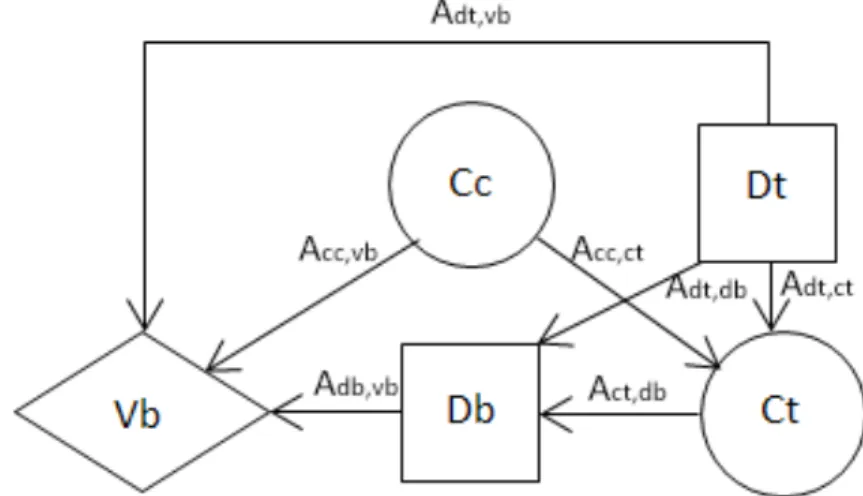
Figure 4: Influence diagram for the simplified version of the Car Buyer problem. Ccrepresents the car’s condition (good or bad),Dtis a decision node for whether to do the test or not, Ct is a chance node for the test result (positive or negative),Db is a decision node for whether to by the car or not and Vb is value node for the total cost.
The diagram graph G is defined as G =< N, A >, where N = {D, C, V}, with subsets D, C and V defined as
D={Dt, Db} (the set of all decision nodes) C ={Cc, Ct} (the set of all chance nodes) V ={Vb} (the set of all value nodes) and the set of all arcs A as
A={Acc,vb, Acc,ct, Adt,db, Adt,ct, Adt,vb, Act,db, Adb,vb}
Direct successors (Si) and direct predecessors (Pi) for each node respectively are defined as
SCc ={Ct, Vb}; PCc ={ } SCt ={Db}; PCt ={Cc, Dt} SDt ={Db, Ct, Vb}; PDt ={ } SDb ={Vb}; PDb={Dt, Ct} SV b={ }; PV b={Cc, Db, Dt}
In accordance with [Shachter, 1986, p.874] arcs Acc,ct, Adt,ct,Adt,vb,Acc,vb and Adb,vb would be classified as conditional arcs, i.e. arcs that indicate conditional influence.
Arcs Adt,db and Act,db are informational arcs and indicate informational influence.
Note that conditional arcs do not imply time precedence or causality, but proba- bilistic dependence. Informational arcs do imply time precedence, which means that
“... uncertainties or decisions at the tails of such arcs have been resolved before the decisions at the head of the arc must be made” [Shachter, 1986, p.874].
In [Howard and Abbas, 2015, p.315-317] a different classification of arcs (arrows) is suggested, where an arc from a decisions node into a chance node is called an influence arrow (arc), and an arc from one chance node into another chance node is referred to as a relevance arrow. An influence arrow from A into B implies that decision A may have influence on the probability distribution of B. A relevance arrow from A into B implies that B is conditioned by A and may be relevant to A.
In accordance with this classification, arc Adt,ct is an influence arc and Acc,ct is a relevance arc.
In accordance with the formal definition of influence diagrams as presented in [Shachter, 1986, p.875], the presented diagram can be considered:
• proper; for a decision maker familiar with the problem and the syntax of influence diagrams, there should be no other way to interpret the diagram but as intended.
• oriented since it contains a value node (Vb) representing the final outcome of the decision.
• regular, since it contains no cycles, all of the decision nodes are connected in a directed path, and the value node Vb has no successors.
Most of decision tools supporting influence diagrams handle influence diagrams as decision nets. The concepts of Bayesian nets and decision nets as a special type of Bayesian nets are explained in sections 3.2 and 3.3, respectively.
3.1.1 Semantic Rules for Influence Diagrams
Semantics is defined as the study of the meaning of linguistic expressions, and applies to both natural and artificial languages. While the syntax of a language provides rules for how expressions are built up in a particular language, semantics provide rules for building meaningful expression units in a language and the rules for combin- ing them into larger meaningful expressions. In the context of influence diagrams, we deal with a simple artificial language consisting of 4 symbols for nodes (rectan- gular, oval or circular, double-oval or double circular and diamond-shaped) and an arc (arrow) symbol denoting relations between nodes. The syntax of the language is very simple. For example, an expression consisting of two nodes connected with an arc is a syntactically correct expression. Obviously, in order for an expression to be semantically meaningful, it has to be syntactically correct, but not all syntactically correct expressions are meaningful. For example, an expression consisting of three nodes connected in such way that they form a cycle is syntactically correct. It is not meaningful, though, since cyclic relations are not allowed in an influence diagram, i.e. a graph containing a cycle has no meaning in the context of influence diagrams.
We consider the rule that cyclic relations are not allowed in influence diagrams a semantic rule.
This study does not aim to account for all semantic rules for influence diagrams, but to analyse and compare the chosen computer programs with respect to some of the rules that are considered relevant in the context, namely i) how they comply with the rules for regular influence diagrams as given in [Shachter, 1986], and ii) if and how they comply with the free-will condition.
3.2 Bayesian Networks
In [Jensen and Nielsen, 2007, p.32-35] a Bayesian net is defined as a net consisting of the following:
• A set of variables and a set of directed edges between them.
• Each variable has a finite set of mutually exclusive states.
• The variables together with the directed edges form an acyclic directed graph.
• To each variable A with parents B1, ..., Bn, a conditional probability table P(A|B1, ..., Bn) is attached.
It is important to note that the definition of Bayesian net does not refer to causality and that there is no requirement that the links in a Bayesian net represent causal impact [Jensen and Nielsen, 2007, p.34]. This is important in the context of using decision networks as a special case of Bayesian networks for solving influence dia- grams.10 As presented earlier, the relation between two stochastic variables (chance nodes) in an influence diagram is not one of causality, but one implying proba- bilistic dependence or independence between variables. This issue is addressed in [Howard and Abbas, 2015, p.148-154] where the authors introduce the concept of a relevance diagram as a network consisting of a set of variables and a set of directed links between them implying relevance rather than causality.11 This distinction is important since it aims to make clear the symmetric nature of the relationship be- tween two stochastic variables. If A and B are two chance nodes and there is an arc from A into B, then the arc implies not only that A is relevant for B, but also that B is, or might be, relevant to A.
A relevance diagram is a representation that primarily highlights irrelevance rela- tions between uncertainties and represents the knowledge of a decision maker based on his/her current state of information [Howard and Abbas, 2015, p.148]. That im- plies that relevance between two variables is not absolutely given, but depends on
10The term decision network is sometimes used as a synonym for influence diagram. In this study the two terms are considered distinct and the term decision network refers to a decision model with the probabilities assigned. A decision network is by definition an influence diagram, while an influence diagram may or may not be a decision network.
11The termrelevance diagram is often used to refer to influence diagram, i.e. the two terms are considered synonyms. In this study the termrelevance diagram is used to denote a representation of relevance relations between uncertainties, as in [Howard and Abbas, 2015]. A relevance diagram thus has no decision nodes.
the knowledge or the preferences of the decision maker. For example, the relevance between traffic accidents and alcohol consumption may be taken as obvious by one decision maker in a certain context, while it may not be recognized by another decision maker in the same or a different context.
In figure 5 a relevance diagram for Age(A)/Alcohol Consumption(AC)/Traffic ac- cidents(TA) is given. Based on the current state of knowledge, the decision maker considers age relevant for alcohol consumption and age relevant for traffic accidents, but assumes no relevance between alcohol consumption and traffic accidents.
Figure 5: Relevance diagram showing that there is a mutual relevance between age and alcohol consumption and between age and traffic ac- cidents, but there is no mutual relevance between alcohol consumption and traffic accidents.
Given new information (statistics showing that drivers under the influence of alcohol are more likely to cause a traffic accident, for example) the decision maker would construct the relevance diagram as shown in figure 6.
Figure 6: Relevance diagram showing that there is a mutual relevance between age and alcohol consumption, between age and traffic accidents and between alcohol consumption and traffic accidents.
A Bayesian network in its simplest form is a probabilistic model of a relevance di- agram. For the relevance diagram in Figure 5, each node has zero or one parent node. The probability table for node A is then given, P(A). The probability ta- ble for node AC is given as P(AC|A) and the probability table for node TA as P(TA|A). The diagram shown in Figure 6 is slightly more complex, as the node TA has multiple parents. The probability table for node AC is again given as P(AC|A).
For the node TA, as pointed out in [Jensen and Nielsen, 2007, p.33], conditional
probabilities P(TA|A) and P(TA|AC) alone tell us nothing about how the impacts from A and AC interact. The probability table for node TA is thus calculated as P(TA|A,AC).
3.3 Decision Networks
A decision network can be defined as a Bayesian network extended with decision nodes and value nodes, i.e. a network that can evaluate a modelled influence dia- gram. Evaluating a net representing an influence diagram (a decision net) is not as straight-forward as solving a regular Bayesian net, though. One obvious prob- lem is how decision nodes are to be handled if a successor chance node is updated?
There are a number of different approaches to and techniques for evaluating deci- sion nets. In [Bhattacharjya and Shachter, 2007] the authors propose an algorithm to evaluate influence diagrams by converting them to arithmetic circuits. Algo- rithms working directly on influence diagrams have also been developed, but the most common is a two-steps approach, where the influence diagram is first mapped to a corresponding decision tree, and then in step 2 solved as a tree structure ([Howard and Matheson, 2005, Qi and Poole, 1995, Jensen and Nielsen, 2007]). How- ever, the details of solving algorithms are not relevant for this study and will not be analysed here.
4 Results and Analysis
Three computer programs for evaluation of influence diagrams are analysed and compared: Netica, Hugin Expert and PrecisionTree.
Both Netica and Hugin Expert are powerful decision support tools based on Bayesian nets. With their graphical and rather intuitive interface, the tools are easy-to-use programs for working with Bayesian networks and decision networks. The creation of decision nets is simple, with different options to assign probabilities. Those may be entered manually, defined in the form of equations or (in Netica) read in from data files. Probabilistic models in both programs may be explored by operations such as reversing individual links of the network, removing or adding probabilistic dependencies, optimizing one decision at time, etc.
PrecisionTree is a Microsoft Excel extension that is primarily aimed at working
with decision trees. However, it includes routines for construction and evaluation of influence diagrams, which is why it is included in this study.
How each of the compared tools comply with the general semantic rules for influence diagrams is analysed in section 4.1.
Section 4.2 consists of two parts. Section 4.2.1 gives a short introduction to asym- metric decision problems and a brief overview of the most important issues when solving an asymmetric decision problem with influence diagrams. The results of the analysis of each tool with respect to the issue are presented in section 4.2.2.
How the compared tools address the arc reversal functionality is analysed in section 4.3.
4.1 Complying with the semantic rules for influence diagrams
The first aspect that is being examined is how flexible the different tools are when creating an influence diagram. In section 3.1 we have seen that there are some formal semantic rules regarding the structure of a proper influence diagram. In this part of the study the compared tools are analysed with regard to whether or not they comply with the semantic rules for regular influence diagrams as defined in [Shachter, 1986, p.875] (4.1.1) and how the free-will condition is handled (4.1.2).
4.1.1 Complying with the rules for regular influence diagrams
According to [Shachter, 1986, p.875], an influence diagram is considered regular if it satisfies all of the following conditions:
1. the directed graph for a diagram has no cycles 2. the value node has no successors
3. there is a directed path that contains all of the decision nodes The performed tests show the following with respect to rule 1:
• Creating a cyclic graph is not permitted in Netica, and it is detected in edit mode. However, it lets the user define a cycle-causing relation, but the error message is triggered and shown in the messages window. When trying to compile the network, the program ends in an error message saying that the network can not be compiled because it contains a cycle.
• Hugin Expert handles the case by not letting the user define a relation that would introduce a cycle. In that way Hugin Expert avoids attempts to compile a net containing a cycle.
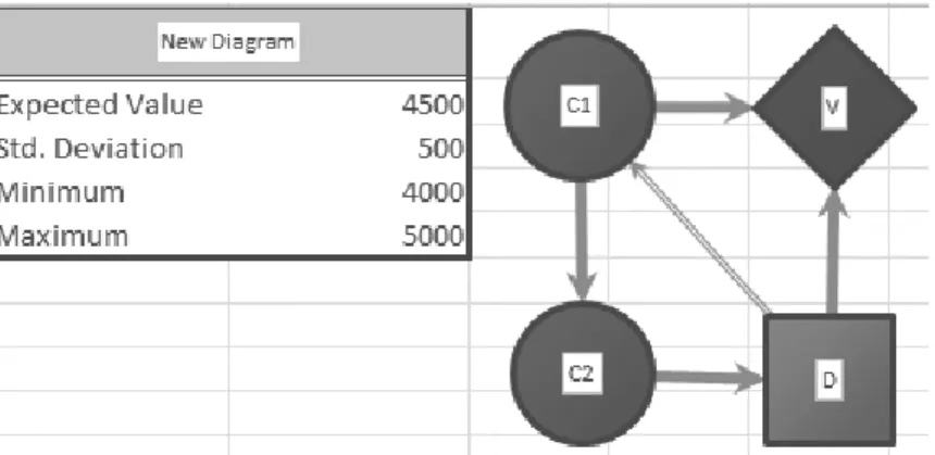
• PrecisionTree seemingly allows creating a cycle, if the cycle-closing arc is de- fined as of type structure. Defining the type of an arc is a feature that only PrecisionTree of the three compared tools has. When adding a relation (arc), its type of relation can be defined as either value, timing orstructure, or any allowed combination thereof. Figure 7 shows an example where C1, C2 and D are connected in a way that, at least on the presentational level, creates a cycle and therefore contradicts the very definition of influence diagrams as directed acyclic graphs. If the diagram was to be analysed in the generic context where the type of an arc is implicitly given as conditional or informational, depend- ing on whether it goes into a decision node or a chance node, this would be considered a flagrant violation of one of the main rules for influence diagrams.
In the generic context, arc C2-D represents a relation from a chance node to a decision node, i.e. is aninformational arc. C2 is aninformational predecessor of D, which means that the value of C2 as well as the value of all of its prede- cessors, which includes C1, are known to the decision maker when decision D is being made. The conditional link D-C1 makes D a direct conditional prede- cessor of C1. Interpreted in accordance with the rules for influence diagrams, this relation between C1 and D means that the value of C1 is observed first after the choice D is made, and the choice made in D influences the value of C1 which is clearly contradictory.
In PrecisionTree the cycle-closing arc D-C1 has a different meaning, being defined as of type structure. If an arc coming out of a chance or a decision node is defined as of typestructure, for each possible value of the decision or the variable one of 5 alternative effects may be chosen: symmetric, skip node, go to payoff, force or elminate. None of these five alternatives includes either the conditional or the informational relevance, and the predecessor node (in this case D) has no impact on the probability distribution for the successor node (in this case C1). The relation is purely structural, meaning that, depending on the choice made in D, the structure of the decision problem would be left as it is, or it would be changed in accordance with the chosen effect for the arc. Since the arcs defined as of type structure do not imply conditional or informational
relevance, they should be left out if the diagram is meant to function on the relation level only, i.e. if the goal is to only show the dependency between variables and decisions (see [Howard and Matheson, 2005]). If the diagram is meant to operate on the function and the number level as well, the structure arcs can be considered a very powerful feature. In section 4.2.2 we will see how this feature can help us with the issues related to asymmetric decision problems.
Figure 7: PrecisionTree seemingly allows creating influence diagrams that contain cycles.
The tests show the following with respect to rule 2 (in a regular influence diagram, the value node has no successors):
• Netica and Hugin Expert handle this issue in a similar way as they handle cycles. Netica allows creating a child node to a value node, but generates an error when compiled; Hugin Expert even here handles the case in edit time.
Even PrecisionTree handles this issue in edit-time12and does not allow creating a child node to a value node.
Regarding rule 3 (there is a directed path that contains all of the decision nodes) the tools are tested on the influence diagram representing a trivial problem. The problem is presented as follows:
X is out for a new car. The car X is considering might be in a good shape or in a bad shape, with the same probability, 50%. X might get a discount
12Actually, in PrecisionTree, there is no edit time in the right sense. All the changes to a diagram are compiled on-the-fly without having to explicitly call the compile function.
for the car, but it is not certain. The probability is 50% that he/she will.
X is also considering the option to borrow some money but he/she does not really need to - he/she has some savings. Should X buy the car?
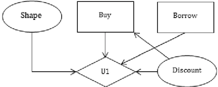
Note that the problem definition does not contain all the information needed to solve the problem, but that is irrelevant in the context. Furthermore, the problem description is not completely logical, but it suits the purpose of the test. The influence diagram for the problem is shown in Figure 8.
Figure 8: The influence diagram for the incomplete Car Buyer problem
We can see that the two decisions do not have any impact on each other, yet both of them influence the total utility U1. There is no direct or indirect relation between the two decisions, which means that the diagram can not be considered regular. The tests show the following:
• Hugin Expert and PrecisionTree do not address this issue. Creating influence diagrams that contain decision nodes that are not connected by a directed path is allowed and the values for the different scenarios including the “loose”
nodes are calculated, regardless whether a decision made in a loose node have any impact on the total utility or not.
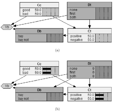
• Netica handles the issue by adding links in order to regularize the diagram. In this particular case, a link from Buy into Borrow is added. Netica makes an assumption that the temporal order of decisions represented by decision nodes is the same as the order of creation of the nodes. Since the node Buy was created first, and since the link from Buy into Borrow does not violate any semantic rules, the link is added (see Figure 9). Now that the link is added, Netica analyses the diagram and assumes that the information coming from the Discount node is relevant for the Borrow node, since it is relevant for the
Buy node that precedesBorrow and hence provide the informational input for it.
(a)
(b)
Figure 9: (a) The original influence diagram for the incomplete Car Buyer example; (b) Influence diagram for the incomplete Car Buyer example after being regularized.
Consider another example: let’s say that we’ve created the influence diagram for the simplified Car Buyer problem as defined in section 3.1, and that we’ve forgotten to add a link from Dt into Db. Despite the node Db being created first, Netica adds a link from Dt into Db keeping the intended semantics of the diagram. This might seem as an advanced AI algorithm running in the
background, but the explanation is rather simple. Namely, Netica realizes that adding the Db-Dt link would violate the no-cycles rule and chooses the only remaining alternative - adding the Dt-Db link.
(a)
(b)
Figure 10: (a) The original influence diagram for the simplified Car Buyer example; (b) Influence diagram for the simplified Car Buyer example after being regularized.
The feature itself (adding the arcs) may be considered useful, as it clearly points out conceptual errors that the user might have missed. However, defin- ing the relations between decision nodes correctly assumes knowledge about the structure of the problem and understanding of the temporal and condi- tional relations between variables, and Netica does not deploy advanced AI modules that would make this possible. Another related feature implemented in Netica and not in the other two tools is removing the arcs that don’t have any impact on the outcome of the problem. An example is shown in figure 11.
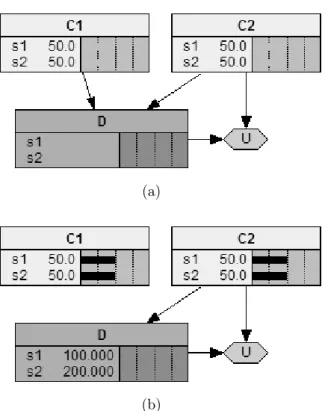
(a)
(b)
Figure 11: (a) Influence diagram in edit-mode (pre-compile). Chance node C1 is a predecessor of D, but it does not influence the outcome, since it does not influence value node U; (b) When the influence diagram is compiled, Netica removes the arcs representing relations with no effect on the outcome, in this case arc C1-D.
4.1.2 Handling the free-will condition
Another interesting issue when evaluating computer programs for influence diagrams is how the free-will condition is handled. The term free-will condition is used here to denote the fact that the consequences of a decision cannot be observed before the decision is made. This simply means that we can not know the outcome of nodes that are successor nodes to a decision node before the decision is made. Say that we have a chance node C that is a direct successor to a decision node D. The relation between D and C is conditional, meaning that the probability of C is conditioned by (dependent on) the choice made in D. It is then first after the decision in D has been made that we obtain the probabilities for the alternatives in C. If this condition is
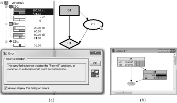
considered, then it should not be possible to lock the probability13for a chance node that has a decision node as predecessor. Hugin Expert handles the free-will issue straight-forward, by not allowing the probability for such a node to be locked. In Netica, the free-will condition is not addressed. The user can lock the probabilities for any chance node in a diagram, even if a node is a successor to a decision node (i.e. can observe/decide the consequences of a decision that has not been made yet).
(a) (b)
Figure 12: (a) The chance node C1 is conditioned by the decision node D1. Hugin Expert does not allow specifying the evidence for C1 if the specified evidence violates thefree-will condition. (b) In Netica, locking probabilities is always allowed; if the evidence is specified in conflict with the free-will condition, the conditioning decision (in this case d1) is calculated by the software.
PrecisionTree is not based on Bayesian networks, it does not come with the func- tionality to lock probabilities, thus for PrecisionTree, the issue of thefree-will is not relevant.
13To lock a probability means to set the probability value for one of the alternatives to 1 - to observe the alternative.
4.1.3 Handling barren nodes
In the context of influence diagrams, a barren node can be defined as a non-target node with no successors, i.e. a node that does not influence the result. As such, barren nodes are unnecessary and may be removed from the graph. [Norsys, 2015]
Even though barren nodes do not change the actual state of an influence diagram, a strict definition of the influence diagram states that it must not contain barren nodes. Netica is the only of the three compared tools that comply with this rule and does not allow creating a barren node, or leaving a node barren after making changes in the diagram. Netica handles this issue in the edit mode, so an influence diagram containing a barren node is never compiled. PrecisionTree and Hugin Expert both allow barren nodes and, despite the fact that they don’t influence the results, the probability distributions for barren nodes are calculated when the decision net is compiled. This may be a minor issue, but it is still important: unnecessary calcula- tions are done, and logical or structural flaws are more difficult to detect.
4.2 Handling asymmetric decision problems
A major disadvantage of influence diagrams compared to decision trees is in han- dling asymmetric decision problems. In [Jensen and Nielsen, 2007, p.310-313] an asymmetric decision problem is defined as a decision problem for which the number of scenarios in all of its decision tree representations is lesser than the cardinality of the Cartesian product of the state spaces of all chance and decision variables.
In order to represent an asymmetric problem, we need to add artificial states and for those states define what Smith et al call degenerate probability distributions [Smith et al., 1993, p.281] - we need to symmetrize it.
4.2.1 Symmetrizing asymmetric decision problems
In order to explain the concept of symmetrization of asymmetric decision problems, let us use the following version of the Car Buyer example where we have added the choice of doing one or two tests:
X is thinking about buying a used car. The probability that the car is in good condition is 80%, and the probability that it is in bad condition is 20%.
X expects to earn 60$ if the car is in good condition; otherwise, X expects to lose 100$. Before X decides whether to buy the car or not, X can choose to do one or two tests. The cost of test 1 is 9$, and the cost for both test 1 and test 2 is 13$. The probability that the first test is positive is 90% if the car is in good condition, 40% if the car is in bad condition. If the first test is positive, the probability that test 2 is positive is 88.9% if the car is in good condition, 33% if the car is in bad condition. If the first test is negative, the probability that test 2 is positive is 100% if the car is in good condition, 44.5% if the car is in bad condition.
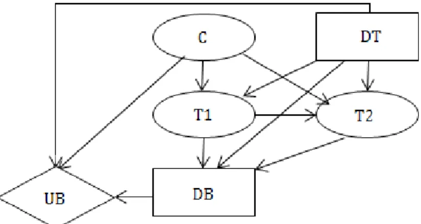
The influence diagram for the problem is shown in Figure 13, where
Figure 13: The influence diagram for the extended Car Buyer example.
• DT: decision – do none, one or two tests
• DB: decision – buy the car or not
• C: chance – car’s condition
• T1: chance - test 1, positive or negative
• T2: chance - test 2, positive or negative
• UB: pay-off
The problem contains two decision variables (DT and DB) and three chance variables (C, T1 and T2) with the following state spaces:
• SSp(DT) = [no tests, test 1, both tests]
• SSp(DB) = [buy, don’t buy]
• SSp(C) = [good condition, bad condition]
• SSp(T1) = [not done, positive, negative]
• SSp(T2) = [not done, positive, negative]
The cardinality of the Cartesian product of the state spaces (or the product of the cardinalities for the referred state spaces) equals 108 (3*2*2*3*3). However, a cor- rectly constructed decision tree for the problem contains only 21 possible scenarios, which makes the example problem a highly asymmetric one.
Let us proceed by analysing the diagram. Decision node DT has no predecessors which means that it is not conditioned by any variable. Chance node C has no predecessors nodes either; it contains given probability values for the car’s condition.
Table 1: The probability values for C.
Good Bad
80% 20%
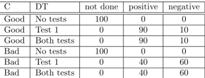
Chance node T1 has two direct predecessors: DT and C. It contains the probabilities for positive/negative outcome for test 1 depending on the car’s condition and the decision made in DT.
Table 2: The probability distribution for T1.
C DT not done positive negative
Good No tests 100 0 0
Good Test 1 0 90 10
Good Both tests 0 90 10
Bad No tests 100 0 0
Bad Test 1 0 40 60
Bad Both tests 0 40 60
If decision DT is to not do the test(s), then there is only one possible outcome for T1, namely not done. Otherwise, the outcome of T1 is one of the other two alternatives (positive or negative).
Chance node T2 has the same two direct predecessors as T1: DT och C. Further- more, it also has T1 as a direct predecessor, and it contains the probabilities for not done/positive/negative outcome for test 2 depending on the car’s condition, the choice made in DT as well as the outcome of test 1. All the possible outcomes for T2 are presented in table 3.
Table 3: The probability distribution for T2.
T1 C DT Not done Positive Negative
Not done Good No tests 100 0 0
Not done Bad No tests 100 0 0
Positive Good Test 1 100 0 0
Positive Good Both tests 0 88.9 11.1
Positive Bad Test 1 100 0 0
Positive Bad Both tests 0 33.4 66.6
Negative Good Test 1 100 0 0
Negative Good Both tests 0 100 0
Negative Bad Test 1 100 0 0
Negative Bad Both tests 0 44.4 55.6
However, not all 18 possible combinations for T1, C and DT have been considered in table 3. In order to symmetrize the problem, wee need to add artificial states for the eight impossible scenarios and then define the probability distribution for each state. This is presented in table 4.
Table 4: The probability distribution for T2 after symmetrization.
T1 C DT Not done Positive Negative
Not done Good No tests 100 0 0
Not done Good Test 1 - - -
Not done Good Both tests - - -
Not done Bad No tests 100 0 0
Not done Bad Test 1 - - -
Not done Bad Both tests - - -
Positive Good No tests - - -
Positive Good Test 1 100 0 0
Positive Good Both tests 0 88.9 11.1
Positive Bad No tests - - -
Positive Bad Test 1 100 0 0
Positive Bad Both tests 0 33.4 66.6
Negative Good No tests - - -
Negative Good Test 1 100 0 0
Negative Good Both tests 0 100 0
Negative Bad No tests - - -
Negative Bad Test 1 100 0 0
Negative Bad Both tests 0 44.4 55.6
Decision node DB has three direct predecessors: DT, T1 and T2. The decision table for all the possible scenarios emerging from predecessors is presented in table 5.
Table 5: The decision table for DB.
DT T1 T2 DB (buy car)
No tests Not done Not done x
Test 1 Positive Not done x
Test 1 Negative Not done x
Both tests Positive Positive x Both tests Positive Negative x Both tests Negative Positive x Both tests Negative Negative x
As we did for the outcomes for T2, we need to add 27-7=20 artificial states denoting impossible conditions for decisions DB. After symmetrization, the table for DB looks like in table 6.
Table 6: The decision table for DB after symmetrization.
DT T1 T2 DB (buy car)
No tests Not done Not done x No tests Not done Positive x No tests Not done Negative x No tests Positive Not done x No tests Positive Positive x No tests Positive Negative x No tests Negative Not done x No tests Negative Positive x No tests Negative Negative x
Test 1 Not done Not done x
Test 1 Not done Positive x
Test 1 Not done Negative x
Test 1 Positive Not done x
Test 1 Positive Positive x
Test 1 Positive Negative x
Test 1 Negative Not done x
Test 1 Negative Positive x
Test 1 Negative Negative x
Both tests Not done Not done x Both tests Not done Positive x Both tests Not done Negative x Both tests Positive Not done x Both tests Positive Positive x Both tests Positive Negative x Both tests Negative Not done x Both tests Negative Positive x Both tests Negative Negative x
Finally, value node UB has C, DT and DB as direct predecessors and contains the following values:
Table 7: The value table for UB.
C DB DT Profit
Good Buy none 60
Good Buy first 51
Good Buy both 47
Good Don’t buy none 0 Good Don’t buy first -9 Good Don’t buy both -13
Bad Buy none -100
Bad Buy first -109
Bad Buy both -113
Bad Don’t buy none 0 Bad Don’t buy first -9 Bad Don’t buy both -13
Adding the artificial states and assigning the probabilities obviously obscures the structure of the problem, but that is not the only issue related to symmetrization.
The complexity of the influence diagram increases as the asymmetry level of the problem increases, which may be an important performance issue for any computer program for the influence diagram evaluation. In our example, the values for 108 different scenarios are calculated for a problem with 21 possible outcomes. For com- plex problems with multiple decision nodes and a large number of chance variables, this may be a difference between calculating outcomes for a few hundreds possible scenarios or tens of thousands impossible, artificial scenarios. This makes handling asymmetric decision problems probably the most important feature of any influence diagram evaluation tool.
4.2.2 Test results
Influence diagrams for the Car Buyer problem as presented in 4.2.1 have been con- structed in each of the three compared tools. Netica and Hugin Expert, the two tools based on Bayesian networks, handle the problem in similar ways. The problem is first symmetrized and then the table entries with all the possible and virtual combi- nations need to be entered. The probability, value and decision tables in both Netica and Hugin Expert have the structure as presented in tables 1, 2, 4, 6 and 7. How- ever, they differ in one important aspect: how the probabilities for the impossible outcomes are assigned.
In Netica, there is an option to mark an alternative as impossible, and for such alternatives, probability values need not to be assigned. Even though this feature somewhat simplifies work with probability distribution tables, it is still rather in- convenient and it is not always easy to single out the combinations that are actually possible. In the Car Buyer example, 10 out of 18 combinations are possible for node T2 (table 4), 6 of which are determined by the problem structure. If the diagram did not have to work with symmetrized problems, we would only need to assign probabilities for 4 out of 18 alternatives. However, the fact that probabilities do not need to be assigned for impossible alternatives suggests that the algorithm is able to single out such alternatives and that they are not evaluated.
In Hugin Expert there is no option to mark an outcome as impossible, which has as a consequence that the probability distribution must be defined even for impossible outcomes. Hugin Expert does not offer the automatic probability functionality, so the probabilities need to be entered manually and it is up to the user to make sure that they add up to 1. Apart from being extremely frustrating, this suggests that Hugin Expert actually does all the unnecessary calculations for impossible scenarios, which is a major drawback. The more asymmetric a problem, the more impossible scenarios there are and the more unnecessary calculations will be performed.
Asymmetric decision problems are handled quite differently and more effectively in PrecisionTree, due to the type-defining feature for arcs that was explained in 4.1.1.
Figure 14: The influence diagram for the extended Car Buyer example created in PrecisionTree.
In our example, we are obviously not interested in the results for T1 (test 1) if our
decision (DT) is to not do any tests. Furthermore, we are not interested in the results for T2 (test 2) if the decision is either to not do any tests, or to do only test 1. While there is no way to handle this efficiently in Netica or Hugin Expert, in PrecisionTree we can avoid symmetrization by adding structure as the relation type for arcs DT-T1 and DT-T2. Adding structure as a type makes it possible to reconstruct the graph, depending on the decision made in DT. By choosing skip node as the effect for the alternative No tests for the arc DT-T1, and choosingskip node for the alternatives No tests and Only test 1 for the arc DT-T2, we make sure that DB does not contain impossible decision scenarios such as Buy the car if the test 1 is not done, test 2 is positive and the option No tests was chosen. Finally, since the car’s condition has no impact to the pay-off if we decide to not buy the car, a structure arc DB-C is added to skip node C for this scenario.
Let us see how this particular decision situation is handled in PrecisionTree. The chance node T1 (test 1) consists of 4 different combinations of predecessor node states, for each of which Test 1 can be either positive or negative:
• Do only Test 1, the car is in good condition
• Do only Test 1, the car is in bad condition
• Do both tests, the car is in good condition
• Do both tests, the car is in bad condition
Figure 15: PrecisionTree: the probability distribution table for T1.
In Netica and Hugin Expert, there are two more combinations:
• Do no tests, the car is in bad condition, and
• Do no tests, the car is in bad condition
that both generate the probability of 1 for the outcome not done in T1. Even for T2 (Test 2) there are only 4 combinations of predecessor node states:
• Do both tests, the car is in good condition, Test 1 is positive
• Do both tests, the car is in good condition, Test 1 is negative
• Do both tests, the car is in bad condition, Test 1 is positive
• Do both tests, the car is in bad condition, Test 1 is negative For each of the combinations, Test 2 can be either positive or negative.
Figure 16: PrecisionTree: the probability distribution table for T2.
In Netica and Hugin Expert, the probability distribution table consists of 18 options, 8 of which are impossible and 6 are always true (see Table 4). The information known to the decision maker when the decision to buy the car or not (DB) is made is one of the 7 plausible information states:
• No tests
• Only test 1; positive
• Only test 1; negative
• Both tests; both positive
• Both tests; both negative
• Both tests; test 1 positive, test 2 negative
• Both tests; test 1 negative, test 2 positive
Figure 17: PrecisionTree: the alternatives table for DB.
In Hugin Expert and Netica, there are altogether 27 different alternatives, 20 of which are implausible (see table 6). Finaly, the last table contains the pay-off value for all 12 possible outcomes.
Figure 18: PrecisionTree: the value table for UB.
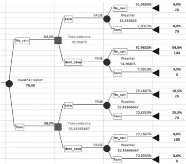
PrecisionTree is the only of the three compared tools that has the functionality to convert an influence diagram to a decision tree. In order for this functionality to be useful, such efficient handling of asymmetric decision problems is critical. The
auto-generated decision tree (Figure 19) consists of 21 different plausible scenar- ios. If PrecisionTree deployed the same solution as Netica and Hugin expert, the generated decision tree for Car Buyer problem influence diagram would have 108 branches/scenarios (Figure 20) of which only 21 are actually possible.
Figure 19: PrecisionTree: the auto-generated decision tree for the Car Buyer problem.
Figure 20: The decision tree equivalent to the influence diagram for the symmetrized Car Buyer problem as constructed in Netica and Hugin Expert.
4.3 Reversing arcs
As we’ve seen in chapter 1, the consistency with the constraints of the information availability is critical when working with decision trees. In a decision tree, the order of nodes must be consistent with the constraints, and this order is in most cases not a natural assessment order. If we can not know X before we know Y, and the infor- mation we have is the probability for Y given X, P(Y|X), then, in order to construct a consistent decision tree, we need to obtain P(X|Y) - we need toswapthe probabil- ities. Those constraints don’t apply in the same way when working with influence diagrams, but for different reasons, we still may need to perform a similar opera- tion - arc reversal. This very important functionality makes working with influence diagrams easier and much more flexible. For example, for a decision problem with imminent cycles it may be difficult to construct a proper influence diagram. Revers- ing arcs makes it possible to overcome the problem without changing the semantic content or the joint probability distribution of the diagram. This is not a straight- forward process, though. Cyclic relations need to be detected and handled by means of arc reversal before a cycle is actually created in a diagram. Reversing one of the arcs creating a cycle in an influence diagram is not possible, due to the restrictions imposed by the theorem for reversing arcs as given in [Barlow and Pereira, 1990, p.26-27].
In [Barlow and Pereira, 1990, p.25] reversing arcs is defined as the probabilistic in- fluence diagram14operation corresponding to Bayes’ formula. The operation, some- times called Bayesian swap, recalculates conditional probabilities and changes the predecessor-successor relation between two stochastic variables (chance nodes) with- out changing the joint probability distribution of the diagram.
Let us use the Car Buyer example as presented in section 4.2.115 to explain the concept more closely. Let one of the nodes in Figure 21 represent the car’s condition, C, and let the other represent the test result for test 1, T1. In (a) we see that the arc between the two nodes goes from C into T1, i.e. we know the probability that the test 1 is positive given that the car is in good condition, P(T1 +|C+). However, what we are interested in is the probability that the car is in good condition given that the test is positive, P(C+|T1+), represented in (b).
14Note that [Barlow and Pereira, 1990] use the termprobabilistic influence diagramfor a graph that in this paper is referred to as a relevance diagram and not an influence diagram.
15In this example, alternative probabilities are used. The probabilities as given in 4.2.1 may cause confusion: P(C+)and the obtainedP(T1+)have equal values, as doP(T1 +|C+)and the calculatedP(C+|T1+)
The following is known prior to test 1:
P(C+) = 0.7 (the car is in good condition)
P(T1+|C+) = 0.85 (test 1 is positive if the car is in good condition) P(T1+|C-) = 0.25 (test 1 is positive if the car is in bad condition)
In accordance with the theorem of total probability, the probability that test 1 is positive is given as
P(T1+) = P(T1+|C+) * P(C+) + P(T1+|C-) * P(C-) = 0.67
By applying Bayes’ rule we can now calculate the probability that the car is in good condition if the test is positive as
P(C+|T1+) = P(T1+|C+) * P(C+) / P(T1+) = 0.89
and the probability that the car is in good condition if the test is negative as
P(C+|T1-) = P(T1-|C+) * P(C+) / P(T1-) = 0.32
(a) P(C+)=0.7; P(T1+|C+)=0.85 (b) P(T1+)=0.67; P(C+|T1+)=0.89
Figure 21: By applying Bayes’ rule we can obtain P(C+|T1+), the prob- ability that the car is in good condition if the test is positive.
Reversing an arc has impact not only on the swapped nodes, but also on their predecessors. Barlow and Pereira suggest the following theorem for reversing arcs [Barlow and Pereira, 1990, p.26]:
An arc [x,y] can be reversed to [y,x] without changing the joint probability function of the diagram if
1. there is no other directed path from x to y
2. all the adjacent predecessors of x(y) in the original diagram become also adja- cent predecessors of y(x) in the modified diagram, and
3. the conditional probability functions attached to nodes x and y are also modified in accord with the laws of probability
Both Netica and Hugin Expert implement the arc reversal functionality in accor- dance with the arc reversal theorem. The functionality is implemented in the same way in Netica and Hugin; all the examples in the rest of this section are done in Netica, but they apply to Hugin Expert as well.
Figure 22 shows an example of arc reversal in a relevance diagram, i.e. a diagram containing chance nodes only.
(a)
(b)
Figure 22: (a) The original relevance diagram; (b) The same diagram with arc D-C reversed.
After reversing [D,C] to [C,D] new arcs are added ( [A,D], [B,D], [E,C], [F,C] ) in accordance with the arc reversal theorem, and the probability tables for affected nodes are modified.16 The modified probability tables for the example are found in Appendix A.
The next example shows the influence diagram for the Car Buyer example with arcs [C,T1] and [C,T2] reversed (Figure 23).
(a)
(b)
Figure 23: (a) The original diagram for the Car Buyer example; (b) The diagram for the Car Buyer example after the two arc reversals.
16Note that the nodes that are connected by the arc that is to be flipped must have same parents, i.e. they must share the set of parents. When the flip is done manually, the parent set for each of connected nodes must be updated accordinglybefore the flip is done.
After the reversal, the arc [DT,C] is added. The probability tables for affected nodes are found in the Appendix B.
PrecisionTree has no support for arc reversal. However, it comes with the function- ality that the other two tools do not have, namely to generate a decision tree from an influence diagram. The generated decision tree may then be used to obtain the modified probability distributions by deploying Bayesian swap on the arc that is to be reversed. All the structural modification needed in order to make sure that the reversal is done properly would have to be done manually, though.
5 Conclusions and Discussion
The influence diagram is an efficient and relatively simple analysis tool. Presenting a decision problem is fairly easy with the influence diagram, due to its high abstraction level. Nevertheless, a high abstraction level is not only positive. Influence diagrams hide most of the details of the decision situation for the user, and while they are suitable for the purpose of presenting the big picture of the decision situation, they may be difficult to interpret on a detailed level, and may be very difficult to evaluate.
In this study three commonly used computer programs for evaluation of influence diagrams are analysed and compared: Netica, Hugin Expert and PrecisionTree. The programs are analysed with regard to three important aspects: how they comply with the semantic rules for influence diagrams, how they handle asymmetric decision problems and if and how they support the arc reversal functionality.
The analysis shows that none of the programs fully complies with the semantic rules that have been used as the comparison criteria in this study. The two programs that are based on Bayesian networks, Netica and Hugin Expert, implement the influence diagram functionality in similar ways, and they deploy similar levels of strictness when it comes to respecting the rules for influence diagrams. In this respect they are both more strict than PrecisionTree. Hugin Expert handles some issues in edit mode that Netica detects first when a decision net is compiled (creating a cycle, creating a successor to the value node). This may not be an important issue for relatively simple graphs, but it might make the difference in performance for complex problems represented by calculation-heavy graphs. One important issue that, unlike Hugin Expert, Netica at least makes an effort to address is the rule that all decision nodes in an influence diagram must be connected by a directed path. As we saw in section 4.1.1, this feature is not fully functional in Netica, but it is still an important feature that may help the user construct a correct influence