PDF Computer Assisted Music Creation

Kurs: DA3005 Självständigt arbete 30 hp 2016

Konstnärlig masterexamen i musik, 120 hp

Institutionen för komposition, dirigering och musikteori

Handledare: Henrik Frisk

Patrik Ohlsson

Computer Assisted Music Creation

A recollection of my work and thoughts on heuristic algorithms, aesthetics, and technology.

Det självständiga, konstnärliga arbetet finns bifogat som partitur.

2

1 C ONTENT

2 Introduction ... 3

2.1 Background ... 4

2.2 Hypothesis ... 5

2.3 Purpose ... 7

3 Method ... 8

3.1 Heuristic algorithms ... 8

3.1.1 Backtracking ... 8

3.1.2 Genetic algorithm ... 11

3.1.3 Practical applications ... 15

3.1.4 Artistic applications ... 18

3.2 Fractal algorithms ... 26

4 Aesthetics ... 31

4.1 Idealism ... 32

4.2 Optimized Intelligibility ... 33

4.3 Mathematical-Music unification ... 34

5 Result ... 36

5.1 Weights Blows Encounters Motions – For Choir ... 36

5.2 Kort Etta – For Accordion and Acoustic Guitar... 40

5.3 KOLOKOL – For Chamber Ensemble ... 43

6 Discussion ... 48

7 References ... 50

8 Appendix ... 53

8.1 Analysis of Per Nörgård’s Symphony no. 3 bar 61-69 ... 53

8.2 PrunedSearch C++ class ... 54

8.3 KOLOKOL score ... 56

3

2 I NTRODUCTION

This work is the text part of the master’s degree in composition at KMH, it complements the artistic part which is supplied in the form of a musical score. Professor Karin Rehnqvist was supervising the artistic part of this work.

This text is partly a testament to my own journey within computer based composition, in particular for algorithmic music creation. It is also an exploration into regions of the thought-world that emerges as a consequence of the method – discussing aesthetic concepts and implications. I wish to introduce concepts that, in combination with an artistic idea, are enabled through the power of technology. I try to holistically approach these subjects – discussing aesthetics, technique, and realization of some musical idea. This, whilst also supplying plenty of notation examples, some code, and illustrations – specifically, to support the explanation of concepts that are uncommon to most students of music.

The text is, on an introductory basis, presenting concepts of both practical and artistic nature involving computer composition. There are a few sections however, that might require the reader to have some familiarity with a computer composition environment or language (such as Max/MSP or SuperCollider).

Not fully grasping these few concepts is not detrimental for the text as a whole, however – some are purposely advanced for completion’s sake, and for inclined readers to return to, if they so wish.

4

2.1 B

The potential of formalizing the compositional process and using programmable machines dates back to early 19^th century. Ada Lovelace, widely regarded as the first computer programmer (Hammerman

& Russell, 2015), stated in regards to Charles Babbage’s mechanical computer, the Analytical Engine:

Again, it might act upon other things besidesnumber, were objects found whose mutual fundamental relations could be expressed by those of the abstract science of operations, and which should be also susceptible of adaptations to the action of the operating notation and mechanism of the engine. Supposing, for instance, that the fundamental relations of pitched sounds in the science of harmony and of musical composition were susceptible of such expression and adaptations, the engine might compose elaborate and scientific pieces of music of any degree of complexity or extent. (L. F. Menabrea, 1842)

Though the field of algorithmic composition may be thought of as one involving computers, the core processes and methods predate the computer age. One early example of this is the pitch-time fractal music of Josquin des Prez – the prolation canon, a common form at the time (15-16^th century) and it involved the superposition of time-scaled and/or offset versions of a melody. This was superimposed on other harmony related rules. The canon itself is a structure built on the rigorous restraints of these rules that project every choice made by the composer that forces a relation to be considered later in time.

In my own work I have gradually transitioned from a non-algorithmic approach to a fully computer based algorithmic practice in the past five years. Initially this transition was done to spend more time on music making and less on fixing mistakes, but I found almost immediately that this shift in method had deeper repercussions in every part of my music creation.

Beyond solving issues there were several important questions brought up through this transition regarding both my own relationship to technology, the role of the composer, and the nature of music itself. By no means will I try to answer all those questions here, but I hope to provoke discussion and perhaps alleviate some common prejudice (Fowler, 1994) on the subject of computer composition.

The Method section of this text will present some potent tools for working with music composition in both practical and artistic ways. Heuristic search algorithms are the methods that lets us navigate huge spaces of possible states such as combinations of notes, durations, or sounds – to find solutions to a particular musical question. It is when attempting to answer such questions that the connection between a musical quality and the musical material is exposed – a significant effort will be put on just how to formulate such questions in this text.

A brief glance on machine learning and in particular deep learning will be included in a gaze forward in to what the algorithmic composition field may become. I will also present the plans for a research project where heuristic algorithms play a key part – the project is dealing with the entire chain from compositional idea to final rehearsals.

5

2.2 H

Composer Per Nörgård made the remark that objects we find and use for artistic purposes (‘objects trouvés’) and the objects belonging to mathematics which is also used for art, that is proportions, the overtone series, and infinity rows – are in kinship to one another.

It may seem surprising that within the same corpus of music, even perhaps within the same work - within the music of the same composer and even within the same work - one encounters on the one hand what have been called 'objects trouvés', that is, objects that have been found, and they don't have to be objects, things, like a box of matches, but also objects like birdsong (in the realm of sound), the roaring of the sea, the crash of waves, wind whistling through the grass, and so on, and on the other hand the composer working with proportions which are called Pythagorean, or the systems of the overtone rows, infinity rows and golden sections. There is, as it were, a Platonic, eternal world, and alongside it this world of immediate presence, of sense experiences. Now for me, these two things are not contrasts. Co-existing at the most, because as far as I can see their kinship is in no way different from that found in music, because in the same way in music we find a high level of abstract order linked to a sound that very much appeals to the senses. And if you remove one of these aspects from music and retain the other alone, then what you have is not music, but amputated music. (Nörgård, Kullberg, Mortensen, Nielsen, & Thomsen, 1999)

Nörgård accentuates the importance of the relation of sense and abstract structure, but there is also the reasoning that these are not contrasts. To some extent the ”eternal world” (Danish: evig verden) of Pythagorean proportions, overtones, and infinite sequences are discovered objects, repurposed for the sake of art or music – in a similar fashion to Marcel Duchamp’s Fountain (Duchamp, 1917).

Now, if music material, form, and every aspect of the music process, would all be “objects trouvés”, harnessed from the eternal world – could a composer be considered a discoverer and not a creator?

What is subjectivity in the composition process when the entire structure of the piece is ”discovered”

and its representation is just a set of practical choices, or even calculations in itself?

The line between representing as, and inventing music, is becoming increasingly blurry in my own work. Is this just a phenomenon of my transition to a programmable digital environment or is music making, at least partially, mathematical structure-representation in sound?

Nörgård’s corpus of music is especially interesting in this case as he has works on both ends of this spectrum – Voyage into the Golden Screen is the epitome for such musical mapping of a mathematical concept, the pitch content of the second movement can be reduced to these formulas:

The infinity row (OEIS: A004718) definition (0 = G over middle C):

𝑓(𝑛) = 𝑓(𝑛 − 2) + (−1)^𝑛+1 [𝑓(𝑛 2⁄ ) − 𝑓(𝑛 2⁄ − 1)]

𝑓(0) = 0, 𝑓(1) = 1 Instrumentation:

flute = 𝑓(𝑛) oboe = 𝑓(4𝑛 + 3) clarinet = 𝑓(2𝑛 + 1) bassoon = 𝑓(16𝑛 + 6) horn = 𝑓(4𝑛) harp = 𝑓(8𝑛 + 7)

With some additional instruments accenting longer wavelengths¹ of the infinity row, such as every 64^th and 256^th note. The piece is in itself a mathematical object represented in sound by Nörgård’s lush instrumentation and phrasing.

1 Nörgård uses the term wavelength (Danish: Bølgelængder) when referring to every nth number in the infinity row. E.g. wavelength 3 would refer to every 3^rd number in the sequence.

6

There is however a significant difference in being mathematical and being mathematically reducible. It is inspiring to imagine that all music has this elegant logic at the core of their being, just hidden in the sounding representation – but even looking at Nörgård’s other music there is obvious ambiguity where formalism ends and experience begin². Sound is described by physics and music structure is to a large extent based on mathematical relations – so every piece could in theory be considered mathematical.

Voyage into the Golden Screen, however, is mathematically reducible in that it can be expressed in a single formula generating the content and structure of the piece. Condensing any piece of any composer in to a simple formula³, is arguably inconceivable⁴.

Now, is there even any reason to believe such a mathematical formula exists for any given piece? If general reducibility of this kind would be discovered, how would this change the way we make and analyse music? This will be furthered discussed in the Mathematical-Music unification-part later in the text.

2 See Appendix – ”Analysis of Per Nörgård’s Symphony no. 3 mm. 61-69”

3 That is a function generating (and simultaneously explaining) all parts of the music, and this whilst being disproportionately simple in definition.

4 This is ultimately a discussion on what a piece is. Is it the emitted sound? The experience of the sound? The score? And what about the interpretation factor, the room, and listener preconceptions – all affecting the experience of the piece? Reducibility would only apply to the domain of conception (e.g. the score’s content, the DAW, or the doodles on a sketching paper), but even there – how would one deconstruct the arbitrarily complex layers of ideas and artistic choices of a piece, into a condensed, mathematical form?

7

2.3 P

There might be no definite answers to the questions stated above – yet I hope to properly introduce these topics and to inspire further research by this text. Also by, in reverse, showing how music can be made on mathematical, or algorithmic ideas – I hope to prove that music and mathematical concepts can share a common ground.

The first part of the text introduces some of the technical concepts such as heuristic and fractal algorithms, that are essential to my own music writing. These concepts are general enough to be applied to practically any musical style, as they are applied prior to, or in concurrence with the conception of the music representation. The text will only present applications that are present in my own work however, that to make it possible to present actual music built on these methods. The structure of the subsections of the Method part is as follows:

 Method description

 Practical applications

 Artistic applications

The second part will deal with some implications of algorithmic music making. Such as the subject of idealism – that is; if it is possible to exhaust the entire search space to find a solution to a musical problem, is there any inherent value (such as beauty) to a perfect solution? We will see that such a solution depends highly on the context of the stated question and the formulation of the question itself. Regarding a solutions value one might have to distinguish between practical and artistic problems but in both cases it is reasonable to favour elegant solutions in contrast to verbose or overly- complicated ones⁵. Now, is elegant the same as beautiful? This remains to be discussed.

In the Aesthetics section we will also discuss the score ↔ musician-relationship and study the effect the visual content of the score has on interpretation. Whilst this could be perceived as non-relatable to the subject of aesthetics it is in the juxtaposition of certain contemporary movements, favouring notational and performative difficulty, and that of optimized intelligibility, a natural outcome of the heuristic workflow (with the goal to maximize simplicity of notation for arbitrarily complex music) – that we might uncover some fundamental aesthetic discrepancies.

These and some other topics discussed in the Aesthetics part are more or less naturally derived from the techniques described in the Methods section and, at least partially, to algorithmic composition as a whole. New possibilities necessitate new theory – these are however only modest, food-for-thought topics, that I hope composers and other inclined readers can experience as inspiring and thought- provoking.

5 By the principle of Occam’s razor, and Optimized Intelligibility, that will be discussed later.

8

3 M ETHOD

3.1 H

When faced with a difficult combinatorial problem whose optimization may be prohibitively expensive, researchers frequently turn to the study of fast heuristic algorithms in an effort to guarantee near-optimal results. (Langston, 1987, p. 539) A practical shortcut taken when solving a combinatorial problem is called a heuristic (from Greek:

εὑρίσκω, "find" or "discover"). Heuristics are employed when a problem involving combinations is sufficiently complicated and it becomes impossible to solve using a brute force method in a reasonable time frame. A classic example is the travelling salesman problem (TSP) stated as follows: Given a list of cities and the distances between each pair of cities, what is the shortest possible route that visits each city exactly once and returns to the origin city?⁶ (Flood, 1956, p. 61)

Here each city added expands the problem exponentially and a full brute force search would start to become impractical already at around 11-12 cities. For 𝑛 cities there would be 1 × 2 × 3 ⋯ × (𝑛 − 1) or (𝑛 − 1)! combinations to try, e.g. for 10 cities: (10 – 1)! = 362880 combinations. Heuristic optimizations and efficient algorithms have made it possible to solve this problem with a million cities (Rego, Gamboa, Glover, & Osterman, 2011, p. 431).

There are several types of heuristic algorithms, from those who simply take shortcuts in a full search effort to those who imitates natural selection and gradually evolve a fitting solution. In general, there are two classes of heuristic methods i.e., those that guarantee an optimal solution and those that do not. When a problem is too large or complicated only an approximate solution might be reasonable to go for – in other cases, such as in the solution of the TSP, a heuristic efficient enough to prune down the search tree to a computable size, could be achieved.

In music there are several combinatorial problems that are similar to the TSP e.g.; deciding accidentals and placing time signatures. We may, as with the TSP, design our own implementation or pick from conventional music praxis to try and solve such problems with heuristic algorithms (see examples in the Practical applications part).

We could also formulate an artistic problem by quantifying a musical quality, defining a problem, and then solving it using heuristics on the resulting search space. One example is finding a combination of sets of pitches (each of size 𝑛) that results in the most occurrences of a specific interval. Another could be finding a combination of a set of sound clips that, when mixed, mimics the spectral structure of a church bell.

In a demonstration I will generate a full instrumentation with notation using: a sample library of instrument recordings, a source sound or sound ideal, a heuristic algorithm, and an exporter. This system can then be extended for microtonal subdivision which also enhances the results (more on this in the Artistic applications section).

3.1.1 Backtracking

A common procedure for solving combinatorial problems is the backtracking algorithm. Imagine picking marbles from some bags and by taking one from each bag you are trying to find a specific

6 Quote from https://en.wikipedia.org/wiki/Travelling_salesman_problem, see reference for the formal problem statement.

9

combination, for example; the set of marbles, one from each bag, that are the largest in total. By picking marbles in a certain order we can make sure that we have tried every combination and indeed found the largest set of stones. To visualize this, we imagine a tree structure where each full branch is a complete combination of marbles as shown in Figure 1.

We pick one marble from each bag until we have reached the last bag, there we cycle through all of its stones, after this we backtrack to the second to last bag and exchange our current stone with a new one from this bag – then cycle through the stones in the last bag again. Once we have picked the last stone from the first bag and cycled through all the stones in all subsequent bags we know that all combinations have been shown and can say for sure what the largest combination of marbles is.

Figure 1, Marble tree (left-to-right) of three bags (dashed), each with two marbles each.

Numbers denoting the order in which the backtracking algorithm picks each marble combination.

This is the full search or brute force method. All combinations are checked with no heuristics for branch pruning, this is not very efficient on a large set of marble bags with many stones in them but it is a good starting point.

As shown in Figure 1, the backtracking algorithm starts at the root of the tree and navigate depth wise down each branch. If we wish to improve the brute force version then each partial solution (Knuth, 1975, p. 125), that is each incomplete combination, could be evaluated against some constraint. If this fails, the algorithm ignores the invalid sub nodes and do an early backtrack up to its parent node to continue with the parents next child node.

A demonstration of the backtracking algorithm for a trivial smallest sum-problem is shown in Figure 2 and Figure 3. We want to determine a sequence of 3 numbers from some groups of positive integers whose sum is the smallest, if the sum is greater than 3 then we have lost.

1

3 4 6

7

8

10 11 13

14

10

Figure 2, Smallest sum < 4.

Partial solution in grey, this won’t continue to check nodes [1] and [2], as the sum is already = 4.

In Figure 2 we see a partial solution/branch where we will check if the constraints are satisfied. Now as 1 + 3 is not less than 4 we see that the constraint has failed. Therefore, we backtrack up the tree and go to the other possible node instead.

Figure 3, Smallest sum < 4.

Sum is less than 4 and it is the bottom of the tree, we found a solution!

There in Figure 3 we see that there exists a solution all the way down the tree, i.e. 1 + 1 + 1. Now in this trivial case we would probably stop searching but if we are not certain that this solution is the best or there might be several optimal solutions we would just output and continue the search.

Large trees where each node have multiple sub nodes could obviously require stricter heuristics. In the smallest sum-problem we could, for example, keep track of the scores of each complete solution and backtrack when a partial solution supersedes the best of these values. This could prune down the tree and improve computation times and it would still find the global optimum/optima.

Now, not all problems are of the smallest sum kind, consider what happens if we want the largest sum instead. Any partial solution would obviously grow when going further down the tree so we cannot, without some prior information about the nodes, use a threshold constraint. Some problems may not be uniformly increasing or decreasing at all which makes heuristic construction tricky or even infeasible⁷.

The backtracking algorithm is well suited for solving a wide array of musical problems as will be demonstrated in the Practical/Artistic applications sections. It works particularly well on smaller combinatorial problems even without strict heuristics. It is easily tailored for optimizations on sequential material such as pitches, scales, durations, number sequences and the like.

My C++ implementation of a version of the backtracking algorithm will be included in the appendix.

7 This could be the case when the nodes represent something non-trivial (e.g. a signal, word, object) or the process of evaluation of solutions is cross-domain, e.g. requires a mixing of signals in the time domain and analysis plus constraint evaluation in the frequency domain.

1

3 1

2

1 1

3

1

3 1

2

1 1

3

<

<

<

<

<

<

<

<

<

<

<

<

<

<

<

<

<

<

<

<

<

<

<

<

<

<

<

<

<

<

<

<

<

<

<

<

<

<

<

<

<

<

<

<

<

<

<

<

<

<

<

<

11 3.1.2 Genetic algorithm

The idea is to start with several random arrangements of components that each

represent a complete but unorganized system. Most of these chance designs would fare very poorly, but some are bound to be better than others. The superior designs are then

"mated" by combining parts of different arrangements to produce "offspring" with characteristics derived from both their "parents". (Peterson, 1989, p. 346)

Genetic algorithms (GA) are part of a larger group of biologically inspired methods called evolutionary algorithms (EA). These procedures are approximate models of actual natural behaviour such as selection, reproduction, and mutation. These methods are used to solve optimization problems, train artificial neurons, or create self-evolving computer programs.

A GA generates a heap of random (complete) solutions (such as marble combinations) and calculates each solution’s fitness, that is, a numerical value signifying how well this particular solution solves the problem (e.g. which marble combination is the largest in total). The most fit solutions are paired and, using a crossover procedure, spliced together to create a new “generation” with a slightly higher average fitness.

The details of the crossover procedure are implementation specific but two common implementations are demonstrated in Table 1. Note that the GA can work on almost any data type and with continuous variables, therefore, designing a custom crossover function might be necessary. Imagine for example what a crossover function on a musical fragment would do – would it splice horizontally, vertically or maybe both?

Crossover at random point

Crossover randomly

Solution 1 (parent): aaaaa Solution 1 (parent): aaaaa Solution 2 (parent): bbbbb Solution 2 (parent): bbbbb Crossover (child): aaabb Crossover (child): ababb

Table 1, Crossover examples.

A GA with just a crossover method would not work very well in practice. Population diversity would decrease quickly, causing the algorithm to “stall” (average fitness not improving by each generation).

This could be mended by 1) including less optimal solutions in the next generation and 2) inducing random mutations on some members of the population. The effect of this is as follows:

1. Helps sustain genetic diversity in the population. In nature, it is not solely the elites that breed the next generation.

2. Simulates the effects of damage, environmental effects and natural variation on individual genes. This also increases variability within the gene pool.

Mutation, as with crossover, is done differently depending on data type and precision. It could be a random alteration applied on all solutions in the population, or just a fraction. It could be a large change, or small. The extent of the mutation could even vary depending on the current generation number – it is all up to the implementer and the problem at hand.

Finally, there are some stopping conditions for the algorithm to seize operation and return the best solution it could find. Some conditions could be superseding a max generations count, improving beyond a fitness tolerance or breaking a time limit (on slow problems).

12

The GA has proven efficient on optimization problems in a surge of areas ranging from scheduling, product design, computational biology (Ławrynowicz, 2008) (Balakrishnan & Jacob, 1996) (Barta, Flynn,

& Giraldeau, 1997), to music and arts (Johnson & Cardalda, 2002).

A significant difference between the GA and the backtrack procedure is that the GA is not guaranteed to return a global optima solution (Forrest, 1993, p. 875). Depending on the starting conditions, crossover and mutation procedures – there is always a risk that the GA gets stuck on a local optimum instead. Another issue is when optima are far apart, solutions might not be able to cross the gap in the search space – this is particularly a risk when the mutation effect is small in comparison to the distances between optima.

These disadvantages are countered by the incredible scalability inherent to the GA – a well implemented algorithm can handle hundreds of variables and achieve high fidelity results.

As mentioned – a GA can be used on many problems of the optimization kind and to end off this section, a GA will be applied to a cross domain fitness problem. Could a ‘tone’ be ‘grown’ in a time domain signal, by looking at it in the frequency domain and evaluate the signal fitness on the spectral content?

The time domain signal consists of 100 samples, these are the variables that the GA will try to optimize.

The GA requires a population of several 100-sample sets, or solutions – each solution in the initial population consists of randomly generated values in the range of -1 to 1. This is the initial setup of the program, now on to the optimization procedure.

As mentioned, before calculating each solutions fitness, the time domain signal needs to be converted in to a frequency domain polar signal. This is done using a discrete Fourier transform which is defined as follows:

𝑋_𝑘 = ∑ 𝑥_𝑛𝑒^{−2𝜋𝑖𝑘𝑛/𝑁}

𝑁−1

𝑛=0

𝑥_𝑛 is our time domain signal, 𝑁 the number of samples in our signal (100) and 𝑋_𝑘 the resulting frequency domain signal over frequency 𝑘. 𝑋_𝑘 consists of complex-valued points in the Cartesian plane but only the amplitude of a particular frequency is of interest in this example – to get this we need to perform a Cartesian to polar conversion (disregarding phase):

𝐴_𝑘 = √𝑟𝑒𝑎𝑙(𝑋_𝑘)²+ 𝑖𝑚𝑎𝑔(𝑋_𝑘)²

𝐴_𝑘 contains the amplitude values for frequency 𝑘. It is on this frequency domain representation the fitness function will be evaluated.

Now, in this example a ‘tone’ will only be ‘grown’ at a single frequency, say 4 Hz, so what is interesting is the value of 𝐴_𝑘 at 𝑘 = 4. What would the time domain signal be expected to look like in the end?

Well, hopefully like a sine wave oscillating 4 times over the 100 sample signal. And what about the frequency domain signal? A pure sine wave of 4 Hz in the time domain would translate to a single straight peak where 𝑘 = 4 in the frequency domain.

The fitness function will not just attempt to maximize 𝐴₄ but it also has to decrease energy at other frequencies, so, the actual fitness formula will be as follows: _max(𝐴^𝐴4

𝑘,𝑘≠4)

A good fitness would mean that the numerator 𝐴₄ is significantly larger than the denominator and the entire expression is approaching infinity.

13

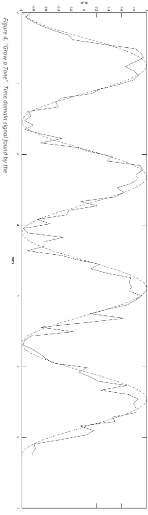
Figure 4, "Grow a Tone". Time domain signal found by the GA and optimal solution in dashed line.

14

Figure 5, "Grow a Tone". Frequency domain representation of time domain signal found by the GA.

The GA was implemented in the Matlab programming environment using the ga function (MathWorks, ga, 2016) with mostly default parameters. By default, ga uses a “scattered” crossover function, that is equivalent to the “Crossover randomly” in Table 1. For mutation, an adaptive function is used by default – when constraints are present. There are only constraints on the range of values (−1 ≤ 𝑥 ≤ 1) but Matlab’s mutationadaptfeasible function guarantees that mutations will not put any solution values outside these bounds.

The only change to the default parameters of ga was population size which was raised to 500 – this proved to be a decent balance between performance and quality on the particular rig this was executed on. After about 500 generations the best solutions in the population were approaching a sine wave, as shown in Figure 4 – the same signal in the frequency domain, the way the GA saw the signal, is shown in Figure 5. Here a clear peak at 4 Hz is apparent and there is not much energy elsewhere.

Obviously, this is not a very artistically interesting problem, but it does demonstrate the power of the algorithm. The GA “figures out” the relationship between a sweeping sine wave in the time domain and a peak in the frequency domain, by just looking at the amplitude at a certain Hz-value, comparing it to the surrounding amplitude level and, gradually evolving a good solution.

It has not been mentioned yet but the time domain sine wave could start at any phase, as this information was discarded in the evaluation process. So there is not just one way for the GA to converge – but infinitely many. The final phase of the sine wave will depend on the initial conditions but with the ability to converge at any phase – it is fascinating that the GA is able to find a particular solution at all.

15 3.1.3 Practical applications

On to some musical examples where the heuristic algorithms outlined above could be used. The two examples will be on general notation issues that are particularly relevant to melodic, serialist, and polyphonic writing. These techniques are, to some degree, present in my own work – as will be further expanded upon in the Result part.

3.1.3.1 Accidentals

When notating a melody, series, or polyphonic part – one will have to decide on a system for setting accidentals. In modal music with no key changes this is not, typically, an issue. If key changes are present there might be some ambiguity on where new accidentals should be introduced – but it is not, unequivocally, a case of right and wrong. Instead, the scenario presented here is when the pitch material is free tonal, atonal, or of unknown structure – as could be the case when mapping a number series to a chromatic scale.

First of all, what could be some of the problems when only picking accidentals of one type (flat or sharp)? In Example 1, a randomly generated 12-tone row with only flat accidentals, some discrepancies are clear. There are augmented intervals from notes 1 and 9, and diminished intervals from note 6 and 7 – this makes the notation a bit harder to read whilst also hinting at a modality that may not be present.

Example 1, All flat 12-tone row.

A neutral representation of the 12-tone row in Example 1 would, preferably, lack augmented or diminished intervals. Also, in an atonal context, it is reasonable to avoid F♭, E♯, C♭, or B♯ – as they impair the readability of the music. So, how could selecting melodically sound accidentals be thought of as a combinatorial problem of the marble-picking kind?

Now, each black key-pitch could be expressed in two ways – sharp low note or flat high note. White key-pitches could, potentially, be written in three ways – for this example only the natural version is allowed. Analogue to the marble problem, we could think of each pitch as a bag of marbles, but instead of stones – each bag contains the different alterations of a given pitch.

Figure 6, Alteration tree (left to right) - first four pitches in Example 1.

The search tree when dealing with accidentals could look relatively minimal, as it only branches on black key-pitches. For longer melodic segments, however, it may turn prohibitively complex as branching exponentially increases the amount of combinations. In Figure 6 the search tree for the first

G♯ A♮ C♮ D♯

E♭

A♭ A♮ C♮ D♯

E♭

16

four notes in Example 1 is demonstrated, and it is clear how this could be navigated in the same manner as the two previous backtracking examples.

Now, what remains are the backtracking constraints – that is, the rules deciding if a partial solution is defunct and backtracking should happen. This could, for example, happen when a branch appends a diminished/augmented interval or reaches a sharp even though all previous music is notated in flats and flat is a possible alteration on the pitch.

The obvious way of filtering out diminished or augmented intervals would be to just backtrack when encountering one – however, this would not guarantee that a solution could be found. Consider note 5, 6, and 7 in Example 1 – there is no way to avoid a diminished/augmented interval without using double accidentals. By this fact we see that terminating an entire branch due to a single diminished/augmented interval is a bad way of guaranteeing good results.

An alternative approach would be to only backtrack on really bad partial solutions, such as when intervals are notated in a different direction from the sounding pitches (e.g. E♯ → F♭). For lesser violations a penalty score would be incremented and the search continued. To improve the heuristics, the penalty score of a partial solution is compared against the best complete solution. If the penalty score surpasses the best penalty score of a previous complete solution, it can be concluded that no optimal solutions exist down that branch – backtracking can be performed.

Example 2, 12-tone row (from Example 1) backtracking results.

In Example 2 the results of this algorithm on the same 12-tone row as in Example 1, are shown. The algorithm was implemented in C++ with the input being the MIDI values of the pitches (middle C = 60) and the output as a vector of number pairs. The first number in each pair being the ordinal (unaltered pitch) and the second number the alteration (-1, 0, or 1).

This is not the only solution, as is clear by the 6^th note, that could just as well be F♯ – fixing the diminished third from 6 to 7, but creating an augmented unison on 5 to 6. Additional heuristics could be imagined, such as incrementing the penalty when a minority alteration is present in a solution – as would be applicable in a locked-down situation such as the note 5-7 dilemma (Example 1 to Example 2). As flats are in minority, over all, penalizing minority accidentals would then result in an additional penalty score on the 6^th note – making F♯ a more viable solution.

For this algorithm to work in a polyphonic setting the heuristics would have to be altered somewhat – making the implementation a bit more complex. This won’t be detailed here but I recommend anyone interested in this to try this out themselves. Were one to allow double accidentals but still want the algorithm to prioritize natural notation then this would have to be arranged correctly in the penalty system.

3.1.3.2 Time signatures

Some problems are perhaps not as common in manual music notation as they are in algorithmic composition – this is true for the following technique. This method should, however, be of interest for anyone writing polyphonic music. The problem this method solves is the following: when generating

17

or composing a rhythmically complex and highly individualized polyphonic texture – how can we ensure that optimal time signatures are selected to maximize on-beat events?

It might seem easy at first to imagine how a backtracking algorithm or GA could solve this problem, but it does in fact introduce some new issues.

1. There are basically infinitely many time signatures – that is if any subdivision of meter and any compound bar structure is accepted (in practice, however, it doesn’t make sense to group below the shortest note duration or create excessively complex compound bars).

2. As time signatures are laid out consecutively, and may be of varying length, there is also a variable number of time signatures in a complete solution. This comes as the total length of the bars has to be ≥ total length of the music, and therefore, the time signature count is dynamic. For the search tree this means that the tree depth, or (complete) solution size, is variable – determined by the content of a particular partial solution.

Besides this, there are no additional complications to what was shown in the accidental problem.

It could be argued that a set of time signatures producing the most on-beat notes is optimal, one might also wish for note ends on beats, as this further simplifies the music-reading⁸. A reasonable conclusion would be that on-beat note ends should be at a lesser priority than on-beat note starts or the algorithm might select an unfit solution.

The particular complications in this example does not hinder using a backtracking algorithm to find an optimal solution – it is, however, inherently easier to implement using a GA (at the possible expense of globally optimal solutions). It is done in these five steps:

1. Calculate start (and end) positions in absolute time of each note in the music to be grouped.

2. Select a number of time signatures, or possible numerator/denominator combinations that will be tested by the GA.

3. Calculate a fixed variable count (number of consecutive time signatures) by:

𝑣𝑎𝑟𝑖𝑎𝑏𝑙𝑒 𝑐𝑜𝑢𝑛𝑡 = 𝑡𝑜𝑡𝑎𝑙 𝑚𝑢𝑠𝑖𝑐 𝑡𝑖𝑚𝑒 𝑠ℎ𝑜𝑟𝑡𝑒𝑠𝑡 𝑏𝑎𝑟 𝑡𝑖𝑚𝑒 .

E.g. if the total music time is 30 quarter notes and the shortest time signature is 3 8 then:

𝑣𝑎𝑟𝑖𝑎𝑏𝑙𝑒 𝑐𝑜𝑢𝑛𝑡 =^{30 4}_{3 8⁄}^⁄ = 20.

Solutions overextending the total music time could be discarded by posing a nonlinear constraint (MathWorks, Nonlinear Constraints, 2016) – or included and the overflow is ignored.

4. The fitness function receives a random complete solution of time signatures that are guaranteed to hold the entire music. The absolute start positions of all beats are calculated from this sequence of measures. Any start (and end) position calculated from the music that does not sit on a beat increments the solutions penalty score.

5. Finally, the GA does its magic of picking from the population of sets of time signatures and gradually improving them until an optimal solution has been found.

8 These rules are good for textural music with little rhythmical accentuation (e.g. György Ligeti’s Lontano), but less adaptable, in general, to homophonic parts where melodic movement would influence measure structure.

18 3.1.4 Artistic applications

Two useful examples were shown on practical⁹ notation issues, but, it is in finding solutions to artistic problems, that I personally believe the potential of heuristic algorithms is the greatest. Two problem statements on two, seemingly contrary composition techniques, will be introduced here in short and later be exemplified in actual music – in the Result part.

Here, I wish to emphasize that the composition techniques presented will not be done so in an overly- faithful way to their inventor(s) – as I would rather explore the full potential of each technique (sans archaic aesthetic restrictions). Arguably, any composition technique is merely a vessel of artistic potential that should not be ignored or praised on any historical preconception. I do find, however, that it is in the undiscovered cracks within this known that the most communicative expression is found.

3.1.4.1 Twelve-tone

I do not have any particular affection for early 20^th century twelve-tone music – yet, I have found that working within a restricted space, such as in dodecaphonic music – can be inspiring at times. A twelve- tone row consists of twelve notes of twelve unique pitch classes. Now, there are guidelines on constructing twelve-tone rows imposed by the inventor, Arnold Schoenberg, that are, in no way, adherent to the technique itself – instead, rather a testimony on his aesthetic views (and, of course, to some of his contemporaries).

The term emancipation of the dissonance refers to its [the dissonance’s]

comprehensibility, which is considered equivalent to the consonance's comprehensibility. A style based on this premise treats dissonances like consonances and renounces a tonal center. By avoiding the establishment of a key modulation is excluded, since modulation means leaving an established tonality and establishing another tonality. (Schoenberg, 1950, p. 150)

Schoenberg wished to get rid of any hints of tonality in his dodecaphonic music and keeping true to his ideals now, would have implications beyond the fundamental rule of having twelve different pitch classes. I will respectfully ignore Schoenberg in these specifics, but, is it possible to take his general concept and search for 12-tone rows that are musically dissolved in other ways?

A natural first step would be to not only have 12 unique pitch classes but also 11 unique intervals. This is commonly referred to as an all-interval twelve-tone row and it has been used extensively by composers Elliott Carter (Childs, 2006) and Luigi Nono (Il canto sospeso, 1955).

Example 3, Luigi Nono – Il canto sospeso. All-interval twelve-tone row.

Typically, intervals of the same size but differing direction are still treated as equivalent and should only happen once. This is demonstrated in Nono’s all-interval row for Il canto sospeso, shown in Example 3. In disjunction with Schoenberg’s dodecaphonic design principles – Nono’s row also has

9 Practical issues are often indiscernible to artistic issues when discussing a specific implementation, the separation is true only from the bird’s eye perspective of this text. That is, that practical application considers more general issues, whilst artistic applications consider a range of specific issues.

19

cadence like movement (such as in note 4-6), that might hint at a tonality. It is, however, the expanding ranges; the dramatic structure of the row – that are the most striking.

Even with all-interval rows it is questionable if the uniqueness of each interval is really a factor in the perceived dissolution of the music. I.e., the row in Example 3 with its powerful trajectory – does arguably not match the punctualist undertones of its unique pitch classes and intervals. Still, there are conceivable situations where an all-interval row, with its lesser internal “connectedness”, is more appropriate to use than an ordinary twelve-tone row – for example in polyphonic music, if repeating harmony is sought to be avoided.

Are there twelve-tone rows that, on an even deeper level, lacks repetition? Even with the questionable perceptibility of the phenomena could, not only, uniqueness in pitch classes and intervals – but also intervals of intervals, and deeper – be of any artistic value?

An ‘interval of intervals’ is essentially just the difference of consecutive intervals. These could be thought of as the growth / shrinkage of the intervals over time and they can be expressed in the ways written on the last two rows (from the top) of Table 2.

Pitch (semitone)

0 1 -1 2 -2 3 -3 4 -4 5 -5 6

Diff 1 1 -2 3 -4 5 -6 7 -8 9 -10 11

Diff 2 -3 5 -7 9 -11 13 -15 17 -19 21

Diff(|Diff|) 1 1 1 1 1 1 1 1 1 1

Table 2, Number representation of all-interval row in Il canto sospeso. |_| denote the absolute values.

In Table 2 a numerical representation of Nono’s row in Example 3, is shown. The top row is equivalent to the pitches (in semitones) from a centre pitch (0), the 2^nd row from the top displays the intervals, and 3^rd and 4^th rows the interval difference – with the 4^th row displaying the difference on the absolute intervals (non-negative). It is clear that the 4^th row is a more tangible representation, as it is observable (in Example 3) that each interval grow one semitone at a time. Yet, when considering the bidirectionality of intervals – row three from the top is the more correct.

Obviously the individual values in the 4^th row of Table 2 are not unique (they are all 1), and if we wrap musical intervals ≥ an octave (e.g. minor 9 = minor 2, major 10 = major 4) and disregard direction – then, the values in the 3^rd row are not unique either. The interval wrapping procedure on the numerical representation is defined by: 𝑊(𝑥) = |𝑥 𝑚𝑜𝑑 12|, where “𝑚𝑜𝑑 12” refers to the remainder after dividing by 12 (retaining the sign of 𝑥), and |𝑥| meaning the absolute value of 𝑥 (removes the sign).

The wrapped numerical representation of the 3^rd row is then: [3, 5, 7, 9, 11, 1, 3, 5, 7, 9]. The first interval difference (originally a falling minor third) is now equal to the 7^th interval difference (originally a falling minor 10) – in this definition, not all interval differences are unique in Nono’s row.

Now, are there even any all-difference twelve-tone rows so that, not only, all interval differences are unique – but also the differences of the interval differences, the differences of the differences of the interval differences and so forth?

It turns out, and the backtracking algorithm can exhaustively prove, that no complete all-difference twelve-tone rows exist (at least not within an octave’s range) – but, it does get very close. First, let’s look at a complete difference matrix (post-wrapping) for Nono’s row:

20 1 2 3 4 5 6 7 8 9 10 11 3 5 7 9 11 1 3 5 7 9 8 0 4 8 0 4 8 0 4 8 4 0 8 4 0 8 4 0 4 8 0 4 8 0 4 0 8 4 0 8 4 8 0 4 8 0 8 4 0 8 0 4 8 4 0

Table 3, difference matrix of the 12-tone row in Il canto sospeso.

Each row in table 3 displays the wrapped values of the unwrapped difference of the row above – the same method used in Table 2, but direction excluded. As shown – the first row (the musical intervals) are all unique – but values are repeating in the 2^nd to 8^th row, which would not be the case in an all- difference twelve-tone row.

Searching for an all-difference twelve-tone row is relatively straight-forward, and similar to what has already been demonstrated on accidentals and time signatures. As in the accidentals-algorithm, I employ a penalty system rather than a terminating one, to ensure that good solutions are not discarded. The penalty score is calculated from the difference matrix – starting at zero, it increments once for each repetition of a number on a row in the matrix.

If all twelve tone-combinations within an octave is tested by the backtracking algorithm using the penalty score for heuristics (see the Accidentals example) – then there are no 0-penalty solutions in the entire search space. More interestingly however, there are exactly four 1-penalty solutions – in fact four versions of one series – that happen to be both all-interval and all-interval-difference twelve- tone rows.

Example 4, Four all-difference 12-tone rows.

Note that each row is transposed to start at C.

Of these four twelve-tone rows shown in Example 4, the second is just the inversion (SI), the third the retrograde (SR), and the fourth the retrograde-inversion (SRI) of the first row (S).

21 9 11 10 7 4 6 8 5 2 1 3 8 9 5 11 10 2 1 7 3 4

5 2 4 9 0 3 8 10 7

7 6 1 9 3 11 6 5

1 7 10 0 2 5 11 8 5 10 2 7 4 1 3 0 9 11

4 3 9 8

7 0 5 7 5 0

Table 4, wrapped difference matrix for “S” in Example 4.

The one penalty – a repeated 6 (tritone) on the 4^th difference level – marked in grey.

The imperfection is on the 4^th difference level (that is the differences of the differences of the interval differences) – a recurring tritone in the, arguably, imperceptible sub structure of the twelve-tone row.

This particular repetition of a tritone is present in all four versions of the row – on this same level.

Of 12 factorial, or 479001600 possible combinations – there is, effectively, just one (imperfect) all- difference twelve-tone row. It is, by this definition – the least repeating and most melodically dissolved combination of twelve-tones in an octave, that could exist. If this quality transfers to the realm of perception is another matter of course, and one that is subject to further study.

3.1.4.2 Spectral composition

The Orchidée and Orchids tools, developed at IRCAM in Paris – are two relatively well known spectral composition software, that generate orchestration suggestions based on the analysis of a sound file (Esling, 2014). Orchids uses an interesting combination of partial tracking, psychoacoustic classifiers, and heuristic search algorithms (Esling, 2014, p. 10), to find a matching orchestration to a source sound – the specifics, however, are not well documented (it is a proprietary software, after all).

I decided to construct my own algorithm for generating an instrumentation based on the spectral content of a given sound clip in late summer 2015. This developed in to a miniature suite of orchestration tools for Matlab – not yet released to the public.

At the core is a synth or sample library generating the audio data to be selected from. Most of the tools will work with any VSTi (virtual instrument), but by default they use the 120 gigabyte orchestra library – EWQL Symphonic Orchestra Platinum. The hosted VSTi is programmatically manipulated to construct matrices of audio data, to be used in the combinatorial problem. The final output is a Lilypond notation file (.ly) containing the suggested instrumentation. This file can be further manipulated in any text editor, or in the freely available Frescobaldi notation software (frescobaldi.org, 2015).

There are specific backtracking algorithms for small instrumentations that can exhaustively search through all instrumentation combinations, and genetic algorithms for medium, to large instrumentations. The tools differ in how they compare the source and generated instrumentation sound. Commonly though, a long-term average spectrum (LTAS) is calculated from a few seconds of audio data (from the instrumentation) – this can then be compared with the data from the source sound.

Several methods for comparing temporal and spectral data are already built-in, but the option of supplying a custom comparison method is also supported. In some of the tools the comparison is done directly on the LTAS of the two sounds, whilst others do various manipulations of the data first. Some built-in methods for comparison sounds include partial distance comparison, regression analysis, and fundamental analysis.

22

Unlike Orchids, one can also specify a sound ideal, in the form of a custom fitness function – which the algorithm will optimize. There are some psychoacoustic helpers, such as perceived amplitude correction (Fletcher-Munson curves), that assist in improving the result. An objective could be designed for, for example, finding the instrumentation that generates the most audible partials, the most even spectrum, or the most energy on the pitch A♭. That way, it is not only useful for sound matching, but for almost any orchestration problem. Some areas this could be used are in spectrally consistent reductions, and adaptations of a piece for a new instrumentation.

All the details on the underlying algorithms driving these tools is beyond the scope of this text, but the toolset was used extensively in composing KOLOKOL a piece I made for chamber ensemble. For the obliged, I suggest reading the part on this piece in the Result section.

Figure 7, Instrumentation algorithm example using a genetic algorithm.

Note that fitness evaluation is done for every solution in the GA population.

A general example of the functionality of these tools is demonstrated in Figure 7. A row in the audio data matrix typically corresponds to a single recorded note of the virtual instrument. The matrix could therefore be organized according to the range of the instruments – so that reconstructing the instrumentation could easily be done from the generated row indices for the matrix¹⁰.

Some of the tools support floating point indices. The integer part of the index could then be used for selecting a sound from the matrix – and the fractional part for calculating a pitch shift on that sound.

10 In reality, the tools create a support structure for easily reconstructing the instrumentation (with pitch and dynamic) from the indices in the matrix (generated by the GA).

23

This way, continuous microtonal solutions could be generated – optional pitch rounding is also possible at any stage of the algorithm (for notation purposes).

The tools are fairly rudimentary, not having any built-in way of dealing with spatialization for example (as is included with Orchids) – but they are programmed on a highly modular principle, meaning that such features could be appended almost anywhere in the algorithm. Spatialization, a custom fitness function, or heuristic could easily be supplied as an extension – via a Matlab file (.m) or anonymous function.

The reasoning behind this extensibility is that the GA is highly sensitive to initial conditions – seemingly small changes in the input data or GA settings, might unexpectedly produce bad results. Being able to control the parameters, extend, and reshape the algorithm for each problem – is therefore of importance on an artistic level.

An interesting phenomenon, that I became aware of when I was writing the piece Weights Blows Encounters Motions for choir, and the piece Variation for 13 musicians (see Example 5) – was the effect of having an extraordinary density of events and voices in close proximity. This seemed, at moments, to have the potential to destroy all perceptive identifiers pertaining to the individual voices, or groups – resulting in the experience of a new, non-divisible sound. The effect is similar to what happens when instruments are playing pitches at harmonic partials from a common fundamental pitch. When balanced perfectly the instruments may no longer be perceived individually, they have become the sum of their parts. An example of this phenomenon, on a harmonic series on E♭ can be heard at the very end of the Prelude to Act I in Richard Wagner’s Parsifal (see Example 6).

Gérard Grisey also described a technique in the article “Structuration des timbres dans la musique instrumentale”, that seem to enable the investigation of this phenomenon. He called it instrumental synthesis – a reconstruction (and extension) of a source sound by orchestrating instruments on the partial pitches of the source spectrum (Grisey, 1991). However, the purpose of this technique was not necessarily to create the illusion of a new sound, but rather to realize a greater theory of spectral harmony – yet, it is reasonable to believe that the perceived illusion of two or more sounds fusing, to create the illusion of a new sound, is in some way a result of overlapping spectra.

A personal goal I set up, in late summer 2015, was to create a music piece consisting only of such sound illusions – never revealing the true sources contained in each polyphonic sound. I started working on the tools presented in the first part of this section, with the hopes of having a workable prototype for the two pieces I would make in the spring of 2016 – one for orchestra, and one for 7 musician Pierrot ensemble. Unfortunately, discovering instrumentations that would generate such sound illusions proved extremely difficult. Having a sound to compare against and then trying to approach its spectral identity, by listing sounds of various instrumentations was one thing – finding a quantifiable measure for the perceived degree of illusion proved a much harder task. There are several potential reasons why it did not consistently succeed in adequately solving the instrumentation fusion problem (IFP), some that I have analysed this far are:

1. Problems pertaining to the heuristic algorithm (GA, backtracking). Resulting in sub optimal solutions even though good solutions existed within the search space.

2. Problems pertaining to the fitness function. Resulting in improper quantifications of relevant perceptual factors in the IFP (several ways of analysing each generated instrumentation’s spectrum was tested).

3. Problems pertaining to the sound generating modules (for the instrumentations). Resulting in an inadequate or incomplete search space.

24

4. Problems pertaining to external factors and method. Perhaps there are no instrumentations from the selected instruments that would create such an illusion. As the algorithm was mainly testing orchestrations of long notes (with some exceptions), perhaps there were solutions using moving pitches.

Finally, I had to settle with a weaker mimetic form of the software (see Figure 7) to do the analysis for one of the pieces (KOLOKOL for Pierrot ensemble). Neither the fusing or mimetic form of the tool was used for the orchestra piece. Yet, the prospect of utilizing illusions of fused sounds in music composition could, like universally unique structures – reveal an entirely new, spectrally surreal, domain of expression.

Example 5, Patrik Ohlsson, Variation for 13 musicians – trills and expressive notes.

25

Example 6, Richard Wagner, Parsifal, Act I, Prelude – ending.

Mainz: B. Schott's Söhne, n.d. (1882). Public Domain.

26

3.2 F

Leaving heuristic algorithms for now and moving on to another central concept for my own work.

Fractal integer sequences, of which Nörgård’s infinity row is one, was the main subject for my bachelor thesis (Ohlsson, 2014). Several methods for generating and composing with self-similar number sequences were exemplified there – therefore, this part will only discuss some recent development regarding self-harmonizing fractal sequences.

First, a clarification – there are many kinds of “fractal sequences”. Any sequence, containing itself as a sub sequence is by definition self-similar / fractal¹¹. Drexler-Lemire and Shallit uses the term “𝑘-self similar” when the sequence recurs on every 𝑘th (for example, every 3^rd) element (Notes and Note- Pairs in Nørgard’s Infinity Series, 2014, p. 11) – this is the case with Nörgård’s infinity row, and it is the definition used in this text.

Now, what does self-harmonizing mean in this context? Looking at the infinity row of Nörgård, one of its defining properties is the exact recurrence of the sequence on every 4^th, 16^th, 64^th, and so on, element. This means that two musicians playing this exact same pitch sequence – one on 16^th notes and the other on quarter notes – would result in them playing unison intervals on all concurrent notes.

Also, a third musician playing the inversion of the sequence on half notes – would play in unison to the others as well.

This is pretty remarkable in itself, yet I wondered – could the cross-voice interval be something else than unison on simultaneous notes? Could series be discovered that recur on musical thirds, or even has a changing relationship to the original voice? Searching for such a sequence could possibly be done through heuristic algorithms, but a more straightforward way is possible if we revisit the original definition of Nörgård’s infinity row.

𝑓(𝑛) = 𝑓(𝑛 − 2) + (−1)^𝑛+1 [𝑓(𝑛 2⁄ ) − 𝑓(𝑛 2⁄ − 1)]

This shows that the element 𝑛, for which to evaluate, is dependent on a value found two steps earlier ( 𝑓(𝑛 − 2) ), the interval at the index half the value of 𝑛 ( 𝑓(𝑛 2⁄ ) − 𝑓(𝑛 2⁄ − 1) ), and a sign changing function ( (−1)^𝑛+1 ). New values depend on prior values, that themselves depend on prior values, and so forth.

Now, a 𝑘-self similar sequence could simply be constructed by picking 𝑘 random numbers, iterating over all other indices 𝑛 = 𝑘 ⋯ 𝑚 − 1 and looking up the value on index ^𝑛_𝑘 on every 𝑘th value. All other values could just be picked at random, as is demonstrated in Example 7.

Example 7, Plain k-self-similar sequence for k=3, constructed from random chromatic pitches.

Sequence recurring on every 3^rd value, highlighted above the staff

11 Consider the sequence of numbers that result from counting 1 ⋯ 𝑛 for each number 𝑛 on the number line in order, i.e. 𝑠(𝑚) = 1, 1, 2, 1, 2, 3, 1, 2, 3, 4, 1, 2, 3, 4, 5 ⋯ (A002260, in the OEIS). If we remove the first occurrence of each number; 1, 2, 3, 4 ⋯, in 𝑠(𝑚) – this will return the very same sequence 𝑠(𝑚) again. This can be repeated indefinitely.

27

The sequence in Example 7 only displays self-similarity on one level, that is, every 3^rd value from the starting point. In this way it is a fairly uninteresting sequence, any value could occupy each “random”

slot so there is a fundamental arbitrariness to this entire process. So, how can several levels of self- similarity be achieved? What would a level be?

A level of self-similarity can be thought of as a 𝑘-power-scaling at a particular offset in the sequence, where the original sequence is recurring (in Example 7 on every 3^rd,with offset 0). In Nörgård’s infinity row the full sequence recur transposed, and/or inverted – on any offset value if 𝑘 is a power of 2 (> 1) (Ohlsson, 2014, p. 14). This means that, even if we start at say the 26^th value in the series and take every 4^th value on to infinity, this sequence would already have occurred starting at offset 26 4⁄ (rounded), i.e. index 7, 8, 9, 10 ⋯ in the row.

𝑠(𝑛) = { 𝑎,

𝑏_𝑚 𝑠(𝑛 𝑘⁄ ) + 𝑐_𝑚, if 𝑛 = 0;

if 𝑛 mod 𝑘 = 𝑚.

𝑚 = 0 ⋯ 𝑘 − 1

A general method for constructing 𝑘-self similar sequences like Nörgård’s row is shown above, the variable 𝑎 is the starting value of the sequence 𝑠(𝑛), 𝑏_𝑚 is the coefficient of a