Study on optimal train movement for minimum energy consumption

(1)

School of Innovation, Design and Engineering

Study on optimal train

movement for minimum

energy consumption

Master thesis work

30 credits, Advanced level

Product and process development Production and Logistics

Panagiotis Gkortzas

Commissioned by: Erik Dahlquist Contact person (company): Kevin Babr Tutor (university): Erik Dahlquist Examiner: Sabah Audo

(2)

[2]

ABSTRACT

The presented thesis project is a study on train energy consumption calculation and optimal train driving strategies for minimum energy consumption. This study is divided into three parts; the first part is a proposed model for energy consumption calculation for trains based on driving resistances. The second part is a presentation of a method based on dynamic programming and the Hamilton-Jacobi-Bellman equation (Bellman’s backward approach) for obtaining optimal speed and control profiles leading to minimum energy consumption. The third part is a case study for a Bombardier Transportation case. It includes the presentation of a preliminary algorithm developed within this thesis project; an algorithm based on the HJB equation that can be further improved in order to be used online in real-time as an advisory system for train drivers.

Keywords: Optimal control, train energy consumption, dynamic programming, Hamilton-Jacobi-Bellman equation

(3)

[3]

ACKNOWLEDGEMENTS

I would like to thank all of the people that helped me throughout my studies in Sweden, my family, friends and colleagues. I would also like to thank people that helped me with this project, Professor Erik Dahlquist and Fredrik Wallin.

Special thanks to Markus Bohlin; this project would never be possible without his valuable help.

Special thanks also to Kevin Babr and Bombardier Transportation Västerås for their help and support during this last semester of my studies.

Finally, I would like to thank my professors during my studies in MDH, especially Professor Sabah Audo for all of the support during the last two years.

(4)

(5)

[5]

Figures

Figure 1: Example of a discrete time problem: going forwards………20

Figure 2: Example of a discrete time problem: going backwards………21

Figure 3: Cylindrical rolling movement……….24

Figure 4: Derivation grade resistances………..……25

Figure 5: Train modes based on power………...28

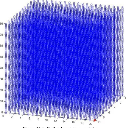
Figure 6(a), (b): Optimal cost-to-go matrix………..38

Figure 7(a): Transitions from a point leading to final time slice………..43

Figure 7(b): Possible transitions from a point inside the matrix - general case………43

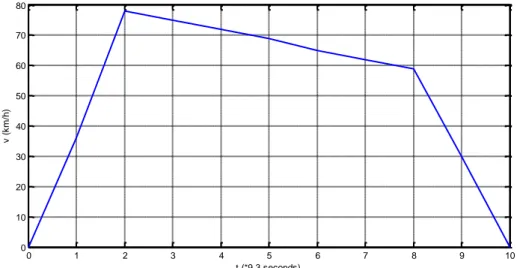
Figure 8: Optimal speed profile for state (0,0,0)(whole trip)……….56

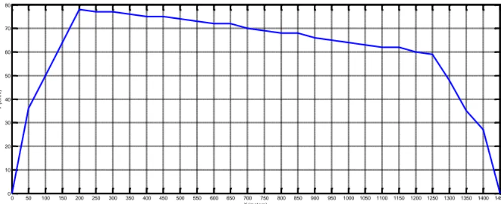
Figure 9: Speed profile for state (0,0,0) based on distance………..57

Figure 10: Optimal speed profile for state (1,4,30)………...57

Figure 11: Optimal speed profile for state (2,3,30)……….58

(7)

[7]

Figure 15: Optimal speed profile for state (6,15,35)………..61

Figure 17: Total distance covered for 30 cases………..64

Figure 18: Optimal speed profile for initial state (0,0,0) and total trip time 200 sec………72

(8)

[8]

1. INTRODUCTION

1.1. Background

In our days, almost all of the companies are concerned about going “green”, making their products/services and their whole function range more environmental-friendly. This is happening due to many reasons. These reasons may have to do with legal issues, since most of the developed countries have already legislated on this direction and have already put limits to the companies regarding parameters like waste, resources, emissions and energy.

Apart from this, there are many other reasons why the companies are moving to this direction. Generally it can be said that taking measurements and moving to an environmental-friendly direction results in a win/win situation for environment, customers and the companies. The scope of this thesis is not to point out these benefits. These are mentioned because exactly these issues and concerns are the reasons for which this project was started.

A transformation of this type for a company usually affects all the range of functions; from the most obvious ones, like waste management, to more complex fields like remanufacturing.

One of the most important aspects of this issue that must be taken under consideration when doing this transformation is energy consumption. It is known that generally the energy resources have been violated by humanity especially during the past century. The last decades there have been many studies pointing out this violation and introducing new ways for energy saving in all the aspects of today’s life; from everyday life functions (e.g. green houses) to complex systems (like energy saving systems on research projects).

Almost all of today’s companies have concerns about reduction of energy consumption. Reduction of energy consumption might refer to the energy consumed during production operations, supply chain-transportation and/or the energy consumed during functioning of the products after sales.

Especially in public transportation, there is a big need for lower energy consumption. The main reason why it is urgent to reduce the energy consumption as much as possible in transportation is that a vast percentage of earth’s population are using public means of transportation which results in this consuming a significant amount of energy. Public transportation means are also used for the transportation of raw material, finished and unfinished products. It is a mean of transportation that is used by many companies in different parts of their functions. This means that, by finding ways to make the public transportation more environmental friendly and by reducing the energy consumed in transportation, a series of benefits will occur firstly for the environment and humanity as a whole, secondly financial benefits for the countries and/or the companies that are responsible for these functions and thirdly

(9)

[9]

for the companies that are providing these environmental, energy-saving solutions because they will be preferred to others in the market.

Exactly for these major reasons, but for other minor reasons as well, there are lots of studies made on this field with different approaches but all with the same scope; meeting the demands (customer satisfaction, satisfying the timetables etc.) with the lowest amount of energy consumed possible.

Bombardier Transportation, as a worldwide leader in the rail-equipment manufacturing and servicing industry is highly concerned about environmental issues in general and more specifically in energy-saving systems in trains.

This thesis project was started as the first part of a bigger long-term project. The whole project has a view to result in an online advisory system for train drivers that will lead to minimum energy consumption. No matter what might have happened during the trip, any delays or other problems that might have occurred, the advisory system that is to be developed will be able to provide the best solution, the control input series that will lead in minimum energy consumption meeting all the requirements as long as this is possible.

By now, there has been great progress in energy-saving techniques for train trips but, most of these systems are offline, which means that they give a speed and control profile that leads to minimum energy consumption from the start of the trip. The major drawback of these techniques is that they do not take under consideration all the random parameters that might affect the trip. This obstacle is surpassed by using an online system like the one presented here, which gives an answer based on a current state that the train is in.

1.2. Problem formulation

The problem to be solved in this thesis is train movement planning for minimum energy consumption. Another way to state this problem is what is the optimal speed profile of a train in a specific line for minimum energy consumption and how can this get further improved in order to be able to be used online as an advisory system for train drivers.

1.3. Aim and Research questions

As mentioned above, this thesis project is the start of a bigger project which means that, everything was started from zero point. This means that in the start many different approaches to the problem were considered until the method that was used was decided. This project’s main aim is to build an algorithm that will calculate the speed profile of a specific train in a specific line that leads to minimum energy consumption. The aim is not an accurate algorithm (since this is not possible in the time given), but a preliminary algorithm on which an accurate program that can be used in real time as an advisory system for train drivers can be based. Some research questions that were to be answered were:

- How should the energy consumption of a train be calculated? What approach should be used since there are different ones?

- What is the method that should be followed for obtaining train optimal speed profile in this project since there are many different ones?

(10)

[10]

- How can a system that can be used online (in real-time) be developed?

- What is the process (logical steps) that has to be followed to obtain optimal speed profile and control series?

1.4. Project limitations

The biggest limit of this project was the time available. Since it is the start of a bigger research project, the expectations were to find a suitable approach to the problem, analyze it and make a working algorithm that can be used in real time.

The algorithm developed is general and can take a number of factors into account, including electric losses, altitude resistances, curve resistances etc. However, in this thesis, only rolling resistances were modeled in detail due to time restrictions.

The aim of this project was mainly to provide an algorithm that can be developed further and result in an accurate advisory system.

The algorithm gives results regarding the trip between two successive stops. This means that the weight load of the train is fixed, given by data from Bombardier and does not change during the trip.

The penalties in the dynamic programming algorithm when a state is not possible, like not being in the end of the line at final time, are just big numbers and have not been picked according to real measurements. Either ways it is impossible to translate for instance the cost of “being late” in energy cost. The penalties issue is something that also needs further research.

Thus, the energy costs that the algorithm is returning may not be fully accurate, but respectively the results are both logical and useful.

(11)

[11]

2. RESEARCH METHODOLOGY

In this part of the report the research methodology followed in this project will be presented. This thesis project includes two main types of research; a literature review and a case study. The literature review can be considered as a part of the case study. This thesis project uses quantitative methods of research. This section of this thesis report will be divided in two chapters; the first chapter will include reasoning on why this project is purely quantitative while the second part will describe the characteristics of this case study and the modes of generalization and reasoning used in this report.

2.1. Qualitative or quantitative?

The research method used in this project is purely quantitative. To support this statement, the general characteristics of quantitative research procedures will be compared to the respective characteristics of the presented project thus identifying similarities and proving that this project is using quantitative research methods. The general characteristics of quantitative research are given by Johnson(2007).

a) Scientific method

The scientific method in quantitative research is deductive or “top-down”. Deductive methods have been used in this project as well, the researcher tests hypotheses and theory with data.

b) View of human behaviour

The human behaviour in quantitative research as well as in this project is regular and predictable. This comes in contrast with qualitative research where the human behaviour is unpredictable, fluid, dynamic, situational and personal.

c) Most common research objectives

The research objectives of this thesis project are in general description of the case and the theory, explanation of the methods used and application of theory and prediction of the results that would be obtained in case this theory was applied in practice. These are the most common research objectives of quantitative research in general as well (Johnson, 2007)

d) Focus

The main focus in quantitative research which is also the main focus of this thesis project is in a narrow-angle target and testing specific hypotheses.

(12)

[12]

After specific assumptions were made, a specific hypothesis/case was made and tested in this project.

e) Nature of observation

In quantitative research there is always an attempt to study behaviour under controlled conditions. This is the method of observation in this project as well, where the conditions of the problem formulated are fully controlled (parameters of track, train and method) and, under these conditions, the behaviour of the train is studied.

f) Nature of reality

The nature of reality here in this project as well as in general quantitative methods is fully objective. What is observed is generally accepted and understood.

g) Form of data collected

In quantitative research the form of data collected is quantitative data based on precise measurement using structured and validated data collection instruments.

In this thesis project, the data used have been given by Bombardier Transportation. The source of the data is automatically proving the precision and validity of the measurements and parameters used here.

h) Nature of data

The data used in quantitative research are variables, while in qualitative research is mainly words, images and categories. The data used in this project are variable values like coefficients, masses, train and track data.

i) Data analysis

The data analysis in quantitative research includes identification of statistical relationships and analyzing numerical results while in qualitative research it includes searching for patterns, themes and holistic features.

In the presented project the data analysis is exclusively an analysis on numerical results so, from a data analysis aspect as well this project belongs to quantitative research.

j) Results

The results in quantitative research are generalizable while in qualitative research the findings are particularistic. As far as it matters the generalizability of the results obtained in this project, there is a need to go to

(13)

[13]

a bit deeper explanation. This will happen in the second part of this section (2.2).

k) Form of final report

The form of the final report in quantitative research is statistical report (e.g. with comparison of results, presentation of mean values etc.) while in qualitative research the form is of a narrative report with contextual description and direct quotations from research participants. Based on these, this report belongs to quantitative research from this aspect as well.

From all the above, the conclusion that can be made is that the presented thesis project is a purely quantitative piece of research. In the next chapter the characteristics of this case study will be presented together with the modes of generalization and reasoning associated with the project.

2.2. Case study characteristics

According to Johansson (2003), a case study should have a “case” which is the object of study. The “case” should:

• be a complex functioning unit,

• be investigated in its natural context with a multitude of methods, and • be contemporary.

The complex functioning unit in this project is the train and its movement on a specific line. The case of the train is investigated in its natural context using approximations while the study is contemporary as explained also in the introduction, since energy-saving train movement is of high interest for all the train manufacturers and users.

Robert Stake (1998) as cited in Johansson (2003) points out that crucial to case study research are not the methods of investigation, but that the object of study is a case: “As a form of research, case study is defined by interest in individual cases, not by the methods of inquiry used”. According to this definition this project is purely a case study, since the focus is on a specific case fully explained and defined.

A very important feature of a case study that has to be explained is the issue of generalisation and reasoning. Johansson (2003) states that generalisations from cases are not statistical, they are analytical. They are based on reasoning. There are three principles of reasoning: deductive, inductive and abductive. Generalisations can be made from a case using one or a combination of these principles.

In this thesis project it can be said that both deductive and abductive reasoning has been used. In fact this project is a hypothesis testing where a theory is tested in a case and it is validated; this shows deductive reasoning. The mode of

(14)

[14]

generalisation based on deductive reasoning is going from a hypothesis and facts to the validation of a theory on optimal control. But this project also includes the procedure of synthesising a case; a case is synthesised from facts in the case and a principle, theory (Johansson, 2003). This points out abductive reasoning. The mode of generalisation associated with abductive reasoning is going from facts and a theory to a case (Johansson, 2003). It can be said that this project is mostly based on deductive reasoning and the associated generalisation type with some characteristics of abductive reasoning.

As a conclusion in this chapter it can be said that this project is a case study made using purely quantitative methods and a mix of deductive and abductive reasoning.

The next section of this report is presenting the theoretical framework of the project.

(15)

[15]

3. THEORETIC FRAMEWORK

In this section, the theoretic part of the presented thesis project will be reported. As mentioned above, this project started from zero point and, exactly because of this, a big part of the study was the theoretic research. The first issues that had to be solved were which method for obtaining an optimal solution should be followed and what would be the most appropriate approach for the energy consumption calculation for our problem. The research went through different stages, different types of models were considered until the one regarded as the most suitable for our case was chosen. In this section of the report, only the theory that was finally used will be presented, even though this was only the final part of the theoretic research and other approaches regarding both energy calculation and the solution to the optimal control problem have been seriously considered and studied before ending up to this method.

This section of the thesis project is divided into four chapters. The first chapter is briefly giving some information about optimal control in general. The second part of this section will be a presentation of the theoretic part of the model used in this study, based on dynamic programming. This second part of the theoretic framework will be a presentation of the Hamilton-Jacobi-Bellman equation. A simplified form of this equation was finally used in the algorithm that will be presented later on in this report. In this part, the equation background will be detailed and for the general case problem. In the next section (empirics), the way that this equation was used as a dynamic programming method will be presented so that the reader will understand the approach that was used better.

The third chapter is presenting the model that was used to calculate the energy consumption of the train. This chapter will present the studies that were used as a guide together with the final equations used, regarding the formulas that Bombardier Transportation uses. In the final part of the theoretic framework, the different modes that the train can be in are presented briefly.

3.1. Optimal Control Theory

The optimal control theory is a still growing field of science in our days. Optimal control is a powerful tool that gives the ability to deal with complex control problems. It requires an advanced mathematical and dynamic programming background and is already famous for its adaptability and quality of results.

Todorov(2006) states that optimal control theory is a mature mathematical discipline with numerous applications in both science and engineering. It is emerging as the computational framework of choice for studying the neural control of movement, in much the same way that probabilistic inference is emerging as the computational framework of choice for studying sensory information processing.

Optimizing a sequence of actions to attain some future goal is the general topic of control theory (Stengel (1993); Fleming and Soner (1992) as cited in Kappen(2011). It views an agent as an automaton that seeks to maximize expected

(16)

[16]

reward (or minimize cost) over some future time period. One example that illustrates this is motor control. As an example of a motor control task, consider a human throwing a spear to kill an animal. Throwing a spear requires the execution of a motor program that is such that at the moment that the spear releases the hand, it has the correct speed and direction such that it will hit the desired target. A motor program is a sequence of actions, and this sequence can be assigned a cost that consists generally of two terms: a path cost, that specifies the energy consumption to contract the muscles in order to execute the motor program; and an end cost, that specifies whether the spear will kill the animal, just hurt it, or misses it altogether. The optimal control solution is a sequence of motor commands that results in killing the animal by throwing the spear with minimal physical effort. If x denotes the state space (the positions and velocities of the muscles), the optimal control solution is a function u(x, t) that depends both on the actual state of the system at each time and also depends explicitly on time (Kappen, 2011).

Kanemoto(1980) states that although continuous time problems may be solved by the conventional techniques such as Lagrange's method and nonlinear programming if the problems are formulated in discrete form by dividing time (or distance) into a finite number of intervals, continuous time (or space) models are usually more convenient and yield results which are more transparent. This is exactly the method that was used in the continuous-time problem of train movement. The time space given was divided in finite-number time intervals. Even if this method provides a much easier approach to the problem, it involves some approximations that had to be done. The approximations that have been used will be presented in section four (Empirics).

The general stochastic control problem is intractable to solve and requires an exponential amount of memory and computation time. The reason is that the state space needs to be discretized and thus becomes exponentially large in the number of dimensions. Computing the expectation values means that all states need to be visited and requires the summation of exponentially large sums (Kappen, 2011). This is where the Hamilton-Jacobi-Bellman equation and more specifically Bellman’s backwards approach comes to give the answer. Bellman’s backwards approach is a method that is solving the discrete transformation of a continuous-time system (Papageorgiou, 2010). Since our problem in its roots is a continuous-time optimal control project, the formulation of the general continuous-time optimal control problem was considered as essential to present. The equation referring to the discretized time approximation problem will be presented in chapter 3.2.

3.1.1 Continuous-Time Optimal Control

As mentioned above, our basic problem for the train movement control is a continuous-time problem, for which a discrete-time approximation is used. For this reason, it is essential to explain and present the general continuous-time dynamic system and give an example of a formulation.

Bertsekas(2000) is describing the general formulation of continuous-time optimal control as follows.

(17)

[17] We consider a continuous-time dynamic system

(eq. 1) where x(t) Є Rn is the state vector at time t, ẋ(t) Є Rn is the vector of first order time derivatives of the states at time t, u(t) Є U Є Rm is the control vector at time t, U is the control constraint set, and T is the terminal time. The components of f, x, ẋ, and u will be denoted by fi, xi, ẋi and ui respectively. Thus, the system (1) represents the n

first order differential equations

(eq. 2)

We view x(t), ẋ(t), and u(t) as column vectors. We assume that the system function fi is continuously differentiable with respect to x and is continuous with

respect to u. The admissible control functions, also called control trajectories, are the piecewise continuous functions {u(t) | t Є [0,T]} with u(t) Є U for all t Є [0, T].

In order to be able to deal with the difficulty of this subject, we assume that, for any given admissible control trajectory {u(t) | t Є [0,T]}, the system of differential equations (1) has a unique solution, referred to as the corresponding state trajectory. In a more rigorous treatment, the issue of existence and uniqueness of this solution would have to be addressed more carefully.

We want to find an admissible control trajectory {u(t) | t Є [0,T]}, which, together with its corresponding state trajectory {x(t) | t Є [0,T]}, minimizes a cost function of the form

(eq. 3) where the functions g and h are continuously differentiable with respect to x and g is continuous with respect to u.

Bertsekas (2000) gives also a simple example of formulation of a continuous-time optimal control problem of resource allocation as follows:

A producer with production rate x(t) at time t may allocate a portion u(t) of his/her production rate to reinvestment and 1-u(t) to production of a storable good. Thus x(t) evolves according to

where γ > 0 is a given constant. The producer wants to maximize the total amount of product stored

(18)

[18] Subject to

The initial production rate x(0) is a given positive number.

The problem formulation in the Bombardier case will be explained in section four (Empirics).

3.2. The Hamilton-Jacobi-Bellman equation

Nikovski et.al.(2012) state that optimal control problems can be solved by solving the Hamilton-Jacobi-Bellman equation. In our case, we will use a simplified approach of this equation. The approach that was used in this project will be presented in chapter 4. Even if the approach that was used in this thesis is better to be explained graphically, it is necessary to present the mathematical background of this equation before explaining our approach in a much more simplified way.

Bertsekas (2000) is presenting the Hamilton-Jacobi-Bellman equation as follows:

For the general continuous-time optimal control problem presented in chapter 3.1.1 we will now derive informally a partial differential equation, which is satisfied by the optimal cost-to-go function. This equation is the continuous-time analog of the Dynamic Programming (DP) algorithm, and will be motivated by applying DP to a discrete-time approximation of the continuous-time optimal control problem.

Let us divide the time horizon [0, T] into N pieces using the discretization interval:

We denote

We approximate the continuous-time system by:

and the cost function by

(19)

[19]

: Optimal cost-to-go at time t and state x for the continuous-time problem, : Optimal cost-to-go at time t and state x for the discrete-time approximation.

The DP equations are:

Assuming that has the required differentiability properties, we expand it into a first order Taylor series, obtaining:

Where o(δ) represents higher order terms satisfying , denotes

partial derivative with respect to t, and denotes the n-dimensional (column) vector of partial derivatives with respect to x. Substituting in the DP equation, we obtain:

Cancelling from both sides, dividing by δ, and taking the limit as , while assuming that the discrete-time cost-to-go function yields in the limit its continuous-time counterpart,

we obtain the following equation for the cost-to-go function J*(t, x):

with the boundary condition

This is the Hamilton-Jacobi-Bellman (HJB) equation. It is a partial differential equation, which should hold for all time-state pairs (t, x) by the cost-to-go function J*(t, x), based on the preceding informal derivation, which assumed differentiability of J*(t, x). In fact we do not know a priori that J*(t, x) is differentiable. However, it turns out that if we can solve the HJB equation analytically or computationally, then we can obtain an optimal control policy by minimizing its right-hand-side (Bertsekas, 2000).

(20)

[20]

3.3.1 Description of the HJB equation, forwards and (Bellman’s)

backwards approach

This chapter will be a simpler explanation of the HJB equation and the different approaches regarding forwards and backwards calculations.

It has to be mentioned here that this explanation is based on a lecture by Professor Yi Ma from the University of Illinois. The lecture is included in the course of optimal control and is on Dynamic Programming and the HJB equation regarding discrete systems. The skeleton of the following chapter is taken from this lecture and this is mentioned here because, since this is taken from lecture notes, the description is coded in bullets and had to be further explained by the author of this thesis.

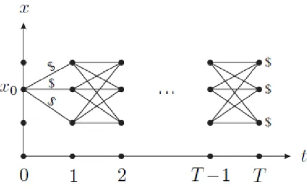
So, according to Ma (2008), Bellman’s dynamic programming approach is quite general, but it’s probably the easiest to understand in the case of purely discrete system. The general form of this equation is:

(eq. 16)

Where is a finite cardinality N, is a finite set of cardinality M (T,N,M are positive integers).

This equation is referring to the forwards calculation. It can be supposed (to show the relation with the train motion problem) that xk is the speed of the train at

step k taken from a pool X of possible speed values, and uk is the control input at

step k taken from a pool U of possible control inputs (like accelerating, coasting etc.). If the forward calculation method was used, this equation means that, at each step, the optimal speed of the next step is obtained by minimizing a cost function, regarding the possible transitions from the current speed and control that can be applied. To explain it better, a simple example (two dimensions-speed and time) will be presented briefly.

Suppose that, at a step k, the speed of the train is xk, the pool of speed values X is

81 values (from 0 km/h to 80 km/h), the control input at a step k is uk and that the

possible control inputs U are accelerating, coasting and decelerating. The way that the forward HJB dynamic programming approach would find the optimal speed for the next step k+1 is the following:

In the start of the track (starting time, k=0) the speed x0=0. At this step it is

obvious that the only possible control input is accelerating (because current speed is zero). Given that the maximum acceleration (speed difference) during one step is known (let’s say that the train engine can accelerate at each step maximum 30 km/h, leveled straight track), the control u0 is accelerating and the possible transitions are

30 for the first step (each transition leads to a different speed value, from 1 km/h to 30 km/h). The HJB equation (eq. 16) would check all the transitions from the given point x0 to the next step k+1 including the non-possible transitions. Then for each

(21)

[21]

transition, an energy cost would be assigned. The way that the non-possible transitions are avoided is assigning penalties for non-possible transitions, so that they will never be considered as optimal. A graphical representation of this simple problem is presented in Yi Ma (2008):

Figure 1: Discrete time: going forwards (Ma, 2008)

Figure 3 shows the most naïve approach where only three transitions are possible. In the example given above these transitions are 80 at each step. Ma (2008) explains that in this method, starting from x0, all the possible trajectories have to be

enumerated, the cost for each must be calculated and then they have to be compared and select the optimal one for the whole problem. The possible sequences that are possible in this problem are actually 81T and to find the cost for each of these sequences T terms have to be added. This means roughly MTT operations. This makes the calculation of the minimum-cost trajectory complicated and almost impossible to define due to the number of calculations needed.

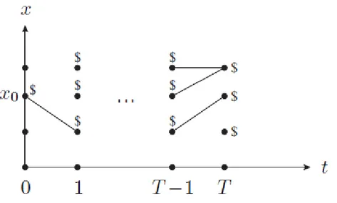
Exactly because of the difficulty of the forwards calculation, the best way to treat this problem is to start from a fixed final state and go backwards in steps (time). In order to use the backward calculation method, at each state a cost-to-go to the ending state must be assigned. At k=T, the terminal costs are known.

The next step is to go to the previous step k=T-1. For each xT-1 all the possible

transitions to k=T must be checked and the minimum one has to be chosen, so as to have the smallest “cost-to-go” (1-step transition cost plus terminal cost). This process must be repeated for all x’s for k = T-2,…,0. When this process is done, an optimal path is obtained from each x0 to some xT. This method is providing the

optimal solutions from each state xk to a fixed final xT that is the desired final state.

The path that will be obtained from this method is unique unless there are more than one paths resulting in the same cost. In the end of the method, for each state xk

an optimal-cost-to-go will be assigned and an optimal trajectory is possible to be assigned. The backward calculation implementation for this simplest case is presented graphically in the following Figure 4.

(22)

[22]

Figure 2: Discrete time: going backwards (Ma, 2008)

A question that usually rises is if the output trajectory is indeed optimal. The answer to this is the principle of optimality for this method.

Principle of optimality: A final portion of an optimal trajectory is itself optimal (with respect to its starting point as initial condition). The reason for this is obvious: if there is another choice of the final portion with lower cost, we could choose it and get lower total cost, which contradicts optimality (Ma, 2008).

What the principle of optimality does is guarantee that the steps that are discarded (going backwards) cannot be parts of optimal trajectories in contrast with the forward calculations where nothing can be discarded (Ma, 2008).

The advantages of the backwards (dynamic programming) approach are (Ma, 2008):

 The computational effort is clearly smaller than with the forwards approach. Furthermore, the backward approach gives an optimal policy for each initial condition (and ). With the forward approach, to handle all initial conditions would require an enormous amount of calculations (T*N*MT), and still it would not cover some states for k>0.

 Even more important is the fact that the backwards approach gives the optimal control policy in the form of feedback: given x, we know what to do (for any k). In the forwards approach, optimal policy does not depend on x but on the result of the entire forward pass calculation.

For the simple two-dimensional example used above since it is known that the final state’s speed must be zero (xT=0), a cost-to-go of zero is assigned at the states

were xT is equal to zero (three states because each state is defined by both speed

and control input). To all the other states at k=T penalty costs are assigned so that it will be sure that the final state chosen will always represent zero speed (the train has stopped).

(23)

[23]

On the next step, we would have to go backwards to T-1 and check all of the states xT-1. For each xT-1 we would have to check all of the possible transitions to the

time “slice” of T-1 and assign the optimal transition and the related optimal cost-to-go to the final time slice of T-1.

In advance, the same method is applied to all the previous time “slices” of 2, T-3, …, 0. In the end, an optimal policy and the related optimal cost-to-go to the end for every possible state would have been obtained. The optimality of the results relies on the principle of optimality presented above.

The example that was presented briefly above is a simplified version of the approach used in this thesis report to solve the optimal energy consumption problem of the case presented in this thesis. The case study that was conducted for this thesis report, together with all the approximations done and detailed explanation of the procedure followed will be presented in section four of this report (Empirics).

3.3. Calculation of energy consumption in trains

The way that the energy consumption is calculated in train motion studies varies regarding both to the approach that is used and in the precision of the formulas used given the approach.

After studying different approaches to this particular field, the most suitable one was chosen to be the calculation of energy consumption based on the driving resistances. This approach is presented to a study conducted by Lindgreen and Sorenson (2005). Their proposed model for the calculation of energy consumption was studied in details and was one of the main guides that led to the model used in the presented thesis project.

Another study that was taken under consideration when the energy consumption equations were being investigated was the doctoral thesis of Lukaszewicz (2001). He used the same main idea on calculating the energy consumption, but his formulas were more detailed, taking under consideration many more parameters and going far in depth in the calculations. This is the most accurate model found in literature, but it is not possible in the time given to collect all the different data needed to apply this model. A similar approach was also used by Jong and Chang (2005) which was also taken under consideration.

Thus, the main idea for the energy calculation formulas was taken mainly by these two studies (Lukaszewicz (2001) and Lindgreen and Sorenson (2005)). For the calculation of the forces though, the formulas given by Bombardier were used instead.

The model presented by Lindgreen and Sorenson (2005) is based on the fact that the energy needed during a specific trip of a train is the energy needed to overcome all the resistances during the motion of the train.

Firstly, all the different driving resistances must be considered. These are presented right below.

(24)

[24]

3.3.1 Driving resistances

It is known that the formula that relates the sum of forces with the acceleration is Newton’s 2nd law:

In our case, a is the acceleration that the train is experiencing when all the different forces F are applied to it. Thus, the connection between the driving resistances and motion is given from Newton’s 2nd law as follows (Lindgreen and Sorenson (2005)): (eq. 4) Where

FM: the locomotive’s traction force at the wheels

Frr: the rolling resistance

FL: the aerodynamic resistance

Frs: the gradient resistance

These four forces are the ones that are most commonly used in different studies on this field. What will actually give us the ability to calculate the energy needed is the traction force needed at the wheels which will result in the train overcoming the resistances and reach the desired acceleration and speed.

m*a is normally called the acceleration force FA, or acceleration resistance. So the

equation (eq.4) becomes:

(eq. 5)

3.3.1.1 Curve resistance

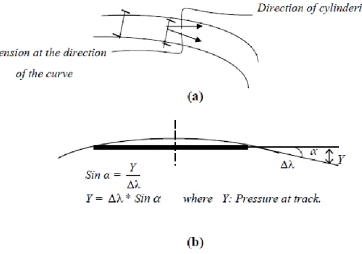
When a vehicle travels on a curve section of its travelway, external forces act on the vehicle. Certain components of these forces tend to retard the forward motion of the vehicle. The sum of these components is the curve resistance. In train motion this resistance depends on the friction between wheel flange and rail, the wheel slippage on the rails (figure 1 (b)), and the radius of curvature (Hoel et.al (2008), p. 107).

Curve resistance is also caused by increasing of tension (direction of tangent of the curvature, figure 1 (a)), increase of pressure on the internal track or external one and possible bad maintenance on the line (Al Helo, n.d.).

(25)

[25]

Figure 3: Cylindrical rolling movement (Al Helo, n.d)

The formula that gives the curve resistance used by Bombardier is:

(eq. 6)

Where

Frk: total curve resistance

mstat: total train static mass (tones)

Cr0, Cr1: constant known values

R: curve radius (m)

3.3.1.2 Aerodynamic resistance

The air in front of and around a vehicle in motion causes resistance to the movement of the vehicle, and the force required to overcome this resistance is known as air resistance. The magnitude of this force depends on the square of the velocity at which the vehicle is traveling and the cross-sectional area of the vehicle (Hoel et.al. (2008), p.103).

The formula presented in Lindgreen and Sorenson (2005) for the calculation of the air resistance in train motion is:

(26)

[26] Where

FL: total aerodynamic resistance (N)

v: train’s speed (m/s)

vwind: the (head) wind speed (m/s)

ρ: air density (kg/m3) CL: drag coefficient

Afr: the frontal area (m2)

3.3.1.3 Gradient resistance

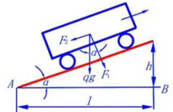
In a rail vehicle rolling along a straight level track, the force component perpendicular to the direction of gravity is zero. However, when the plane of the track is inclined (e.g. when the train runs uphill or downhill), a force component F2 develops parallel to the plane of the track (Figure 2), and in the case of an uphill gradient this component is an additional resistance to vehicle motion (Ding et.al, 2009).

Figure 4: Derivation grade resistances (Ding et.al, 2009)

The equation that gives the gradient resistance is (Lindgreen and Sorenson (2005):

(eq. 8)

Where

FS: total gradient resistance (N)

mtot: train mass (kg)

g: acceleration of gravity (9.82 m/s2) a: angle of the gradient

Δh is the height difference (m) over the horizontal distance (m) And the similar equation that Bombardier uses is:

(27)

[27]

(eq. 9)

Where

Frs: total gradient resistance (N)

mstat: total train static mass (tones)

g: acceleration of gravity (9.82 m/s2) S: gradient (‰)

3.3.1.4 Rolling resistance

Rolling resistance is the sum of the mechanical forces, exclusive of windage and braking, acting to impede the forward motion of a train traveling at constant speed on level track under operating conditions. These have been divided into two parts which are classified "normal" and "abnormal" (Bernsteen et.al, 1983).

Normal Rolling Resistance includes energy losses in the suspension system, hysteresis in the soil beneath the tracks, friction within the bearings, and sliding at the wheel-rail interface.

Hunting, flanging, unequal wheel radii on the same axle, and wheel lift are the most important forms of abnormal rolling resistance. Parasitic energy dissipation in the draft gear caused by grade changes and train handling is another form of abnormal rolling resistance (Bernsteen et.al, 1983).

The formula presented by Lindgreen and Sorenson (2005) for the calculation of total rolling resistance (normal and abnormal) is:

(eq. 10)

Where

FR: total rolling resistance (N)

CR: rolling resistance coefficient

mtot: train mass (kg)

g: acceleration of gravity (9.82 m/s2)

The formula that is used from Bombardier for the calculation of the rolling resistance is:

(eq. 11)

Where

Frr: total rolling resistance (N)

arr, b, c: rolling resistance coefficients (depending on weight load)

(28)

[28]

3.3.2 Energy consumption

Based on this approach there are two main ways to calculate the energy consumption. The first one is based on distance while the second one is based on time.

The energy cost based on distance or time is obtained as follows:

3.3.2.1 Energy consumption calculation based on knowledge of

driving resistance and distance

(eq. 12)

Where Ftot is the sum of the driving resistances as mentioned above.

3.3.2.2 Energy consumption calculation based on power and time

The total power Pe needed can be calculated as (Lindgreen and Sorenson (2005)):

(eq. 13)

Where

Pe: total power (W)

v: speed (m/s)

Ftot: sum of the driving resistances (see above) (N)

based on that the energy consumption is obtained by integrating the total power needed for the total trip time. This gives (Lindgreen and Sorenson (2005)):

(eq. 14)

Where

E: total energy consumption (J) Pe: total power (W)

t: elapsed time (s)

(29)

[29]

(eq. 15)

The model that was preferred for this thesis was the one based on time. The reason for which this model was preferred together with the final formulation will be explained in section four (empirics).

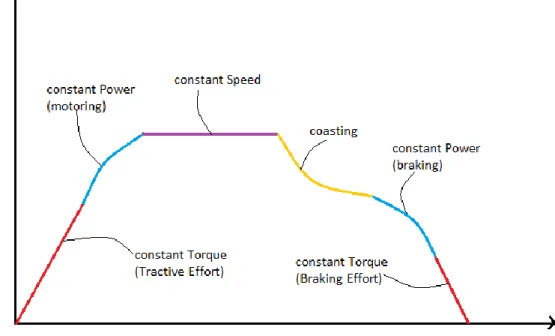
3.4. Train modes

The different modes that the train can be in are six based on the output power of the motor and the motor torque. The output power (P) of the motor is given by:

Where:

P: the output power of the motor T: the motor torque (tractive effort) ω: the motor angular speed

The different modes of the train movement based on speed are shown roughly below:

Figure 5: Train modes based on power

In this thesis project the modes are separated as: accelerating, constant speed, coasting, regenerative braking and mechanical braking. The modes will and the way they are defined will be explained in section four (empirics).

(30)

[30]

4. EMPIRICS

In this section of the presented thesis the steps that have been taken throughout the study will be explained in details. The way that optimal control theory and the Hamilton-Jacobi-Bellman equation were applied to the Bombardier case will also be explained in details. The first part of this section will be a presentation on how the energy consumption formula was obtained from theory regarding the Bombardier case and all the approximations that had to be assumed.

4.1. Driving resistances and energy consumption in the

Bombardier case

4.1.1 Driving resistances

The long-term goal for the whole research project is a detailed model, taking under consideration all the different parameters, which will be able to give optimal advice to the train drivers on the actions they should follow in order to reach to the next station on time with the lowest energy consumption possible, given the current position of the train, the time remaining according to the time tables and the current speed of the train.

Given that this thesis project was time-limited and that the scope of this thesis was not a fully detailed model, but a working model that can be improved further, not all of the resistances have been taken under consideration. The reason why this happened will be explained in the following paragraphs.

When it comes to the curve resistance (resistance associated with the curves (turns) of the track), the ability to calculate it demands a very detailed knowledge of the tracks. This information is available for the line that is under study, but the process of adding these resistances in our calculations is time-consuming and needs to be further studied. This happens because, in order to use the dynamic programming model, the track had to be divided into equal distance intervals. This means that each of these intervals may include different curves, making the process of adding this type of resistances difficult. One way for the curve resistances to be taken under consideration is, for a specific line given, to distribute the curve resistances equally along the position intervals, and collect an approximated energy amount that is needed to overcome these curves. The calculation of this type of resistances, as well as the aerodynamic and gradient resistances, were regarded from the start as a problem that is to be considered and solved later on this project, and are not a part of this study.

(31)

[31]

As far as it matters the aerodynamic resistance, this is generally not taken under consideration from Bombardier. This happens because this type of resistance is depending highly on the weather and is more or less random throughout the year. In fact, even if a detailed and accurate forecast for the wind direction and speed was available, still the calculation of the aerodynamic resistance is almost impossible. This happens because the train is changing direction through the line when taking turns, so the side where the wind is facing the train is changing. It can be said that, since the curve resistances are not taken under consideration, the train is not changing direction along the line, but even if this assumption is made, the aerodynamic resistance will not return realistic results. In order for this type of resistance to be reasonable and represent the real value, the direction of the train against the wind must be known in details. This is the reason why the aerodynamic resistance is not taken under consideration.

The gradient resistance is actually a major factor of the energy consumption formula. Just like the curve resistance, the gradient force needs detailed track data which will need to be further processed in order to be used, because of the method that was used. As mentioned above, for the formulation of the problem, the track had to be divided into equal intervals. Each interval might include different values of gradient, a fact that causes a problem when the gradient resistance is to be calculated. In order for the gradient resistance to be included to the model that was developed, an approximation has to be used. One way to approximate the gradient resistance is to go across the line, starting from the first interval, consider the gradient changes inside the interval and calculate a unique approximated gradient resistance for each interval. The fact that for each position interval, a different coefficient would have to be used would make the formulation of the problem much more complex. This will be understood better after the detailed explanation of the optimal control algorithm that was developed.

The rolling force is the biggest resistance force during the train motion. The coefficients of the rolling resistance equations are different for different weight loads of the train. In this study, the train was supposed to be fully loaded so the rolling coefficients that were used were the ones associated with a train fully loaded. The formula that was used to calculate the rolling resistance in this thesis is the one used by Bombardier (eq. 11).

The acceleration force or acceleration resistance (FA) is coming from Newton’s

second law. In reality, and in the case under study, this force represents the force needed to achieve an acceleration value of a for a train of mass m when no resistances are applied to the train movement. This would be the only resistance in the ideal case of a straight leveled track (no gradient and curve resistances) with no other parameters affecting the train motion.

It has to be mentioned here that, as described in the theoretic background and will be described further later on, the approach used to our problem is a mixture of equal-time and equal-distance dynamic programming model, with a main focus on equal-time steps. This means that the total trip time between the stations under study, had to be divided into equal-time steps. Thus, whenever a calculation has to be done, it is done for a time duration of one time step which will be referred to this text by the term tstep. This is a realistic approach since all of the transitions that are calculated in this project refer to one time step.

(32)

[32]

In this thesis the forces/resistances are calculated as follows: a) Acceleration force FA (for one time step)

(eq. 17)

where the term

(eq. 18) is the equivalent constant acceleration that makes the train experience a difference in speed of for one time step. As mentioned in the previous chapters, this comes from the approximation that for each time step the acceleration is constant and the speed is linear with time for each time step.

b) Rolling resistance Frr (for one time step)

Since the speed is linear with time for each transition (time step), the rolling resistance for each time step can be calculated according to the average step speed which is:

(eq.19)

So the rolling resistance for each time step will be:

(eq. 20)

So, in our case it will be:

(33)

[33]

4.1.2 Energy consumption

From equations (eq. 13) and (eq. 14) taken from theory the total energy consumption of the train can be obtained from:

(eq. 22)

Where

T: total time duration of the trip (for our case is T=93 seconds) Pe: power consumption

Ftot: Total resistances the train has to overcome

E: total energy consumption

Since the speed is supposed to be linear with time for each time step (eq. 22) from (eq. 19) becomes:

(eq.23)

dt is the time step. Given that the total trip time between the two successive stations under study is known the time horizon is discretized into equal time steps. Therefore, dt will be known and replaced by the term tstep. Now (eq. 23) becomes:

(eq. 24)

Where

E: total energy consumption T: total time duration of the trip

Ftot: sum of all driving resistances based on time

tstep: time step/interval (10 equal time intervals for a total trip time of 93 seconds gives a value of 9.3 seconds for each time step)

v(t-tstep): starting train speed of each time interval v(t): final train speed of each time interval

As mentioned in the theoretical background, there are two ways by which the total energy consumption can be calculated; one based on the driving resistances and position and one based on power (which actually comes from the first one since total power is calculated from total driving resistances and average interval speed). In case that the first approach was chosen, it would be easier to include all the secondary resistances in the model. This is a fact because position would be included to the objective function and, for different position values, all the different resistances would have to be added. The problem that arises when using this approach is that the most important constraint which is actually the trip time would have to be calculated from the values of position and speed. This, regarding the

(34)

[34]

resistances and the approximations that have been made, would lead to approximated time values.

An approximation that had to be used is that the speed is changing linearly with time. This made easier the transformation of the objective (energy cost) function, so that the acceleration was translated into speed difference over time. This was also an important reason why the calculation was made based on time instead of position. For every transition in the dynamic programming model the energy cost was calculated, and the position value was calculated from speed difference and time using the appropriate approximations and transformations. This process of calculations will be explained further later on this report.

So, based on these formulas, the energy consumption equation becomes:

(eq.25)

And for one time step (eq. 25) becomes:

(eq. 26)

4.2. Distance/position calculation

As it has been described already, in order for this model to be applied, the trip between two successive stations had to be divided into time and equal-distance intervals. Since the model for the energy consumption that was used is based on time and does not include distance, at every step (transition) that is made in the algorithm the distance covered had to be calculated. The distance covered is easy to get obtained by the ordinary equations of accelerated motion with constant acceleration. The trip under study covers a total distance of 1.51 km. The track is divided into 20 equal-distance steps, so every distance interval represents a distance of 75.5 meters.

Time, distance and current train speed are the dimensions of the 3D matrix that holds the energy cost-to-go, a matrix which is the guide to the optimal control trajectory calculations. Since distance represents a dimension of a matrix, the position values must be integers. This means that every time that the distance covered in one time step is calculated, the result has to be rounded to the closest integer. Thus, a reasonable variation in the total distance covered is experienced, a fact that will be discussed further in the section where the results will be presented.

For a time step transition from state n-1 to state n from the equations of accelerated motion with constant acceleration the position covered can be calculated as follows:

(35)

[35]

And for 1 time step this becomes:

(eq. 27) Where

Xt: final position of the train for one transition

Xt-tstep: Starting position of the train for one transition

vt: final train speed for one transition

vt-tstep: initial train speed for one transition

tstep: time interval for one transition

This is the formula that gives the final position of a transition when the starting position, starting and final speed, and the time step are known.

The way by which these transitions are calculated and the whole philosophy behind this method will be explained further in the following chapters.

(36)

[36]

4.3. Implementation of the Hamilton-Jacobi-Bellman

equation, Bellman’s backwards approach

In this chapter, the process of finding the optimal solution will be explained in details. This part of the presented thesis project will include the following chapters:

1) Introduction to algorithm implementation; planning the algorithm, description of the matrices associated with the program

2) Initialization: fixing the final state, filling the ending time-slice of the cost-to-go matrix, assigning initial penalties

3) Description of transitions leading to the ending time-slice of the cost-to-go matrix

4) Description of all the possible transitions inside the cost-to-go matrix 5) Obtaining the optimal final speed for each matrix element

6) Obtaining the optimal control input for each matrix element

7) Obtaining the optimal speed and control trajectory given the input (current time, position and speed)

4.3.1 Introduction to algorithm implementation

This chapter will be an introduction to the model built during this thesis project based on the implementation of the backwards Hamilton-Jacobi-Bellman equation (dynamic programming approach).

As explained before in this report, the main idea behind our algorithm is to build a matrix that will hold the minimum cost-to-go (to the end of the line and time) for every combination of time elapsed, distance covered and current speed.

After this matrix is initialized and filled backwards, it becomes the basic tool by which the optimal sequence of control inputs and optimal speed values are obtained. The process by which this is achieved will be explained in details.

Apart from the cost-to-go matrix there are two more matrices of the same size as the (cost-to-go) matrix that needed to be generated and used. These are the optimal control matrix and the optimal next time step speed matrix. These two matrices are used in order to make it possible for the program to return results that are easy to understand and make the algorithm results easy to understand by people that are not familiar with optimal control, such most of the train drivers.

This is the main objective of the long-term project as well as for this thesis project. The expected result is an algorithm that can be used online, which requires an algorithm that is running fast, and gives results that can be immediately used by the train drivers. This requires results that are easy to understand and implement.

Study on optimal train movement for minimum energy consumption