VTI särtryck 365A
Utgivningsår 2005
www.vti.se/publikationer
Design
ing an up to date rut depth monitoring
profilometer, requirements and limitations
Leif Sjögren and Thomas Lundberg
Crack measures and reference systems for a
harmonised crack data collection using
automatic systems
Petra Offrell and Leif Sjögren
Reprint from the 2
ndEuropean Pavement and Asset Management
Conference, 21
st–23
rdMarch 2004, Berlin, Germany
The influence of r
oad surface condition
on traffic safety
Anita Ihs
VTI särtryck 365A · 2005
Designing an up to date rut depth monitoring
profilometer, requirements and limitations
Leif Sjögren, Thomas Lundberg
Crack measures and reference systems for a
harmonised crack data collection using automatic
systems
Petra Offrell, Leif Sjögren
The influence of road surface condition
on traffic safety
Anita Ihs
Reprint from the 2
ndEuropean Pavement and Asset
Management Conference, 21
st–23
rdMarch 2004,
DESIGNING AN UP TO DATE RUT DEPTH
MONITORING PROFILOMETER, REQUIREMENTS
AND LIMITATIONS.
Senior Researcher Leif Sjögren and Research Engineer Thomas Lundberg, The Swedish National Road and Transport Research Institute (VTI)
SE-581 95 LINKÖPING/ SWEDEN TEL: +46 13204359, +46 13204395
E-mail: leif.sjogren@vti.se; thomas.lundberg@vti.se
1 Abstract
Sweden has a long tradition in road surface condition monitoring. There are two measures that have dominated the estimation of the road surface condition; namely rut depth and IRI (International Roughness Index). Rut depth is the estimate of unevenness in the transverse and IRI in the longitudinal direction of the road. Deformation or wear that shows up as rut depth are common in Sweden. One big reason is that there is a law to use winter tyres (usually studded) during the winter season. Yet another reason is the actual loads that are transported. To detect differences in wear origin certain specifications is needed to be fulfilled in the design of the monitoring device. This report will deal with findings and conclusions made from years of experience in Sweden. The organized road surface monitoring scheme started in the end of 1970: s. The result is stored in the Swedish PMS (Pavement Management System). Almost all paved roads maintained by the government have been monitored every year. In this paper the result is focused on 10 years of data from one of the seven regions in Sweden. The length of measured roads in this region, Mälardalen is approximately 3000 km per year. A mean transverse profile is stored every 20 meter of measured road. Each profile is estimated from 17 sensors.
We have looked on questions like; have the distance increased between the two wheel tracks during the years? How many sensors are needed and who should they be arranged to best fulfil different missions?
The results from this study show that distance between the wheel tracks has increased. We have also found a possible best specification for design of a rut measuring device.
2 Background
The transverse profile from roads is used as one input to determine the condition of the road. From the transverse profile rut depth is calculated. This measure is much depending on how the transverse profile is measured and what type of profilometer and algorithms to calculate rut depth that is used. This article describes how to best equip a profilometer to measure rut depth.
Road Administrations around the world has, for a great many years in succession, used data from road surface surveys collected by survey vehicles as the basis for maintenance
management on paved roads. Today, this constitutes a substantial amount of the data input supplied to the PMS (Pavement Management System) used by the Swedish Road
The type and priority of used data from road surface surveys is chosen different among the users around the world. The requirements due to climate, traffic, vehicles and road material is different. Actually this is the case even within countries and is also changing during the years. In Sweden studs has been used frequently during wintertime under a long period of years. This has been one reason why transverse evenness expressed as rut depth has been a prioritised road surface measure in Sweden.
The mean transverse profile is the basis for many of the parameters that describe transversal unevenness. Rut depth is defined and calculated using what is called the ”wire surface principle”, which means that an imagined wire is stretched tense across the transverse profile and the greatest deviation from this line measured at a right-angle constitutes the maximum rut depth.
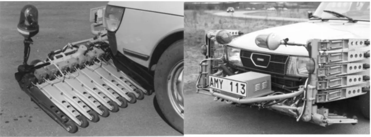
The first Swedish organized road surface data collection started in the seventies. A SAAB Road Surface Tester (RST) was developed and used to collect road surface data. The transverse profilometer consisted of 25 wheels on a bar in front of the car, see figure 1.
Figure 1: SAAB RST, the right picture show the transport position
The 25 wheels and their vertical change due to unevenness across the road were measured and formed a transverse profile. In the eighties the Laser RST that used contact less measuring with the help of eleven lasers, to collect the data, replaced the SAAB RST. One major finding was the possibility to angle the outermost lasers to reach a wider measurement width than the maximum allowed width of a vehicle, see figure 2.
Later requirements improved the system and they are currently using 17 measuring points. Two of the laser, in the supposed wheel tracks was also used to measure the longitudinal unevenness. The displacement of those two lasers defined who to drive laterally on the road to fit in the wheel tracks.
With the change of conditions such as traffic loads, vehicle, material improvements and new type of studs, an investigation was done to find out if the displacement and number of lasers was optimal to satisfy the needs for a stable and objective measure. One hypothesis was that the distance between the rut bottoms has increased. If this was the case a change of either the lateral position when measuring had to be done or a new set up of displacement had to be specified. The investigation led to a number of interesting results. One was the optimal number and placement of measuring points to be used in the transverse profile to calculate the rut depth. For instance it was found that some of the laser points were almost never used when rut depth was calculated. With respect to the data material in the investigation the optimal rut depth configuration has been determined and methods how to determine this has been developed. The investigation has also established algorithms to calculate rut depth.
3 Problem
description
• The first part of the study looked at questions like: What measuring points are used from a transverse profilometer when rut depth is calculated?
• The second part of the study looked at if the distance between rut bottoms have increased during the years. As an extra study we also evaluated if the cause of wear could be identified by looking at the transverse profiles.
• And the last part discusses the design of an optimum rut depth profilometer. How many sensors are needed and who should they be arranged to best fulfil different missions?
4 Method
The first and second part of the study used the following method and data. By using the stored mean transverse profiles and do recalculation of rut depth it is possible to simultaneously save statistics about support points (active reference points) in the profile. The result from road monitoring for the past five years (1998 – 2002) from three of the seven regions in Sweden is summarized. Data from the main roads are used in the study. The amount of data used each year is shown below.
• South of Sweden, region Skåne – 2000 km. • Middle of Sweden, region Mälardalen – 3400 km. • North of Sweden, region Norr – 4000 km.
A mean transverse profile is stored every 20 meter of measured road. Each profile is estimated from 17 sensors.
The third part of the study used approximately 9000 reference profiles from a large number of different road types. The reference profile was measured as described in chapter 4.3. Simulated computer models of different transverse profilometer configurations were used to calculate rut depth from the reference profiles. The chosen configurations can be seen in figure 4.
4.1 Measurement
points
used in rut calculations
In Sweden the rut depth are calculated using the principle called the wire method. The method is used on three sections of the transverse profile, namely the left, right and the complete profile. In this part of the study the effects from the complete profile is considered. Below is an example of the wire method principle.
Supporting point Supporting point Point "max rut"
Figure 3: Wire rut method
The rut depth is the maximum distance between the tensed wire and a measurement point in the profile. In this study all rut depth calculations are based from the twenty metre average transverse profiles. Statistics of supporting and “max rut” points are stored for every profile. The statistics are used to examine who often measurement points are used as support points in the wire rut calculation.
4.2 The change of rut shape characteristics
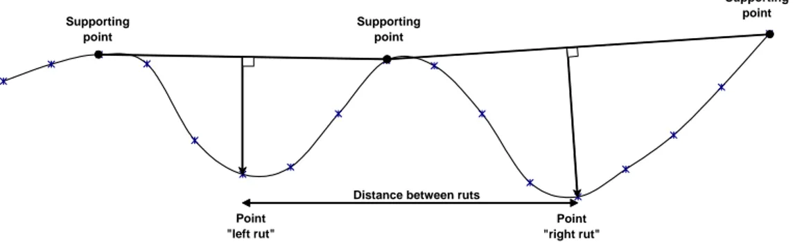
The change (increase) in time of the distance between the rut bottoms has also been studied. This information can be used to determine the influence of traffic and vehicle types on the wear and deterioration of the road surface. The definition of distance between the rut bottoms is explained in the figure below.
Supporting point Supporting point Point "left rut" Point "right rut" Distance between ruts
Supporting point
Figure 4: Definition of distance between rut bottoms
The distance between position of the left and right maximum ruts is calculated. To avoid outliers in this study there are some criteria that has to be fulfilled to include a transverse profile in the analyses. The main purpose is to only include profiles with traditional and distinct ruts. The criteria are as follows.
• The left and right rut depth should be greater than 5 mm. • The maximum rut depth should be greater than 7,5 mm. • The distance between ruts should be greater than 1,3 m.
profile reference data, mainly used as comparison material for measurement vehicles and detailed road studies. The reference data is collected as a continuously measured transverse profile with the VTI-TVP (VTI Cross Profile Scanner). The VTI-TVP is a semi-static reference instrument mainly used at the Swedish procurement of road surface measurements. The vehicle is instrumented with an inclinometer and three lasers of witch one is scanning the transverse profile at a width up to 4 m. A transverse profile including crossfall is collected normally every second metre along the road. The transverse sampling rate is 4 mm.
Figure 5: VTI-TVP reference transverse profile measurement equipment
Simulated computer models of measurement vehicles with different setup
0 500 1000 1500 2000 2500 3000 Transverse distance (mm) 5_1 11 17 25 33 65 15 5_2 17_new 15_new
VTI-TVP reference transverse profile Three different lateral positions with a five point model
-10 -8 -6 -4 -2 0 2 4 6 8 -2 -1.5 -1 -0.5 0 0.5 1 1.5 2 Transverse distance (m) Pr o fi le (mm)
Lateral position - left Lateral position - middle Lateral position - right
Figure 7: Example of lateral position on reference profile for tested measurement vehicle model
5 Results
5.1 Measurement points used as support point in rut calculations
What measuring points are used from a transverse profilometer when rut depth is calculated? In figure 8, 9 and 10 some results from this investigation are presented. One interesting finding is that a number of points are almost never used as active points in the calculations. Two points can especially be identified, one at 1070 and one at 2130 mm. The conclusion is that they should be moved. One can also see that the leftmost rut is sharp and the right most is more smeared out.
0% 10% 20% 30% 40% 50% 60% 70% 80% -100 400 900 1400 1900 2400 2900 Transverse distance (mm) Fr e quen cy ( % )
Left supporting point Point of max rut Right supporting point
0% 10% 20% 30% 40% 50% 60% 70% -100 400 900 1400 1900 2400 2900 Transverse distance (mm) Fre q ue ncy (% )
Left supporting point Point of max rut Right supporting point
Figure 9: Measurement points used in wire rut calculation, region Skåne
0% 10% 20% 30% 40% 50% 60% 70% -100 400 900 1400 1900 2400 2900 Transverse distance (mm) F req ue nc y ( % )
Left supporting point Point of max rut Right supporting point
Figure 10: Measurement points used in wire rut calculation, region Mälardalen
5.2 The change of rut shape characteristics
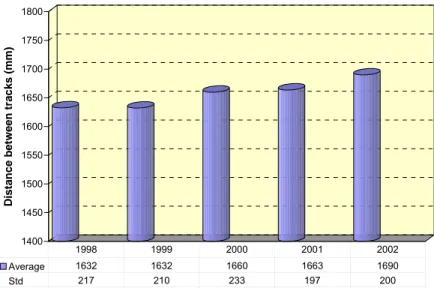
In the second part of the study it can be shown that the distance between the wheel tracks has increased. This can be seen in figure 11, 13 and 15. The increase is in general 10 mm per year.
In figure 12, 14 and 16 the result about what type of traffic causes the ruts is shown. In the last five years ruts caused of cars have decreased from 57% to 41% in the studied regions and consequently ruts caused of heavy traffic have increased from 43% to 59%.
1600 1650 1700 1750 1800 1850 1900 1950 2000 Distan ce b e tween trac ks (mm) Average 1795 1804 1815 1830 1848 Std 221 264 195 197 216 1998 1999 2000 2001 2002
Figure 11: Distance between rut bottoms, region Norr
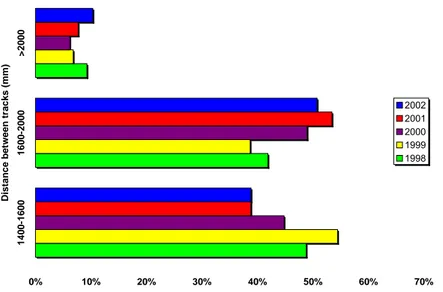
0% 10% 20% 30% 40% 50% 60% 70% 80% 1400-1600 1600-2000 >2000 Distance b et w een tr acks (m m) 2002 2001 2000 1999 1998
1400 1450 1500 1550 1600 1650 1700 1750 1800 D is ta nc e bet w ee n t rack s ( mm) Average 1670 1633 1675 1702 1713 Std 227 202 212 213 223 1998 1999 2000 2001 2002
Figure 13: Distance between rut bottoms, region Skåne
0% 10% 20% 30% 40% 50% 60% 70% 140 0-16 00 1600 -200 0 >2000 Distan ce b et w een tr acks ( mm) 2002 2001 2000 1999 1998
1400 1450 1500 1550 1600 1650 1700 1750 1800 Dis tan ce be tw ee n tr ac k s (m m) Average 1632 1632 1660 1663 1690 Std 217 210 233 197 200 1998 1999 2000 2001 2002
Figure 15: Distance between rut bottoms, region Mälardalen
0% 10% 20% 30% 40% 50% 60% 70% 1 400 -1 600 160 0-200 0 > 2 000 Dista n c e b e tw een track s (m m) 2002 2001 2000 1999 1998
Figure 16: Cause of wear based on evaluation of transverse profile, region Mälardalen
5.3 Designing an up to date rut depth monitoring profilometer
Results from the investigation to find optimum configuration of a rut depth profilometer is shown in figure 17-21.In figure 20 and 21 one can see that 17 to 25 points seems to be optimum if cost per extra point is considered. The rut depth decreases a lot when less than 17 measurement points are used provided that 3,2 m measurement width are used.
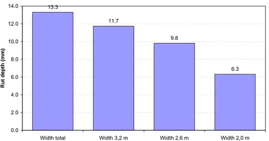
330 cm seems to be a good choice of measurement width for Swedish conditions, see figure 22. The lateral position of the measurement vehicle is as important as the number of sensors, e.g. the driver and operators should be thoroughly educated. This has been evaluated in other tests done in Sweden. Increasing measurement width definitively increases the calculated rut depth (mainly on primary roads). The width must of course be adapted to the situation and type of road.
Rut depth calculated with computer models using 9000 reference profiles 3.47 7.26 9.65 7.95 10.10 10.31 10.23 10.69 10.97 11.39 11.76 0.00 2.00 4.00 6.00 8.00 10.00 12.00 14.00 5 point 2,0 m 5 point 3,2 m 11 point 3,2 m 15 point 2,6 m 15 point 3,2 m 17 point 3,2 m 17 point (new) 3,2 m 25 point 3,2 m 33 point 3,2 m 65 point 3,2 m Continuous transverse sampling 3,2 m R ut de p th ( m m )
Figure 17: Average rut depth from investigated computer models of profilometers
The Influence of Measurement Width on Rut Depth Continuous transverse sampling
13.3 11.7 9.8 6.3 0.0 2.0 4.0 6.0 8.0 10.0 12.0 14.0
Width total Width 3,2 m Width 2,6 m Width 2,0 m
R u t de pt h ( m m)
Figure 18: The influence of measurement width on rut depth when using continuous transverse sampling
The Influence of Lateral Position and Measurement Width on Rut Depth Continuous transverse sampling
0.00 2.00 4.00 6.00 8.00 10.00 12.00 14.00
Left Middle Right
Lateral position
R
u
t depth (mm)
Width 3,2 m Width 2,6 m Width 2,0 m
Figure 19: The influence of measurement width and lateral position on rut depth when using continuous transverse sampling
The Influence of "Number of Measurement Points" on Rut Depth Measurement Width = 3,2 m, Right Transversal Position
0.00% 10.00% 20.00% 30.00% 40.00% 50.00% 60.00% 70.00% 80.00% 90.00% 100.00% 0 5 10 15 20 25 30 Rut Depth (mm) Cu mu la tive freq u e n cy (%)
Cumulative frequency 5 lasers 3,2 m Cumulative frequency 11 lasers 3,2 m Cumulative frequency 17 lasers 3,2 m Cumulative frequency 25 lasers 3,2 m Cumulative frequency 33 lasers 3,2 m Cumulative frequency 65 lasers 3,2 m Cumulative frequency Continuous transverse sampling 3,2 m
Average Rut Depth and Number of Measurement Points Measurement Width 3,2 m 5 11 15 17 25 33 65 0.00 2.00 4.00 6.00 8.00 10.00 12.00 14.00 0 10 20 30 40 50 60
Number of Measurement Points
Ru
t Dep
th (
mm)
Middle Position 'Target Value Middle Position'
Figure 21: The influence of number of measurement points on rut depth at 3,2 m measurement width
The change of rut depth when increasing the number of measurement points from: 17 to 25 is 0,4 mm
17 to 33 is 0,6 mm 17 to 65 is 1,1 mm.
Used Straightedge Length at Different Measurement Width
0.0% 1.0% 2.0% 3.0% 4.0% 5.0% 6.0% 7.0% 8.0% 9.0% 10.0% 11.0% 12.0% 0 200 400 600 800 1000 1200 1400 1600 1800 2000 2200 2400 2600 2800 3000 3200 3400 3600 3800 4000
Required measurement width (mm)
Freq
uen
cy (%)
C
RACK MEASURES AND REFERENCE SYSTEMS FOR A
HARMONISED CRACK DATA COLLECTION USING AUTOMATIC
SYSTEMS
PhD. Petra Offrell SCC/Ramböll RSTIsbergs gata 3, SE-211 19 Malmö/ Sweden Phone +4640105536 / Fax +4640305905
E-mail petra.offrell@scc.se Leif Sjögren
Swedish Road and Transport Research Institute (VTI) SE-581 95 Linköping / Sweden
Phone +46 13204359 / Fax +46 13204060 E-mail leif.sjogren@vti.se
Abstract:
The increased use of automatic systems for crack data collection has created some interesting questions about suitable crack measures. Traditional measures are sometimes unsuitable or even impossible to obtain using automatic data collection. However, the efficient and fast automatic crack data collection has also increased the numbers of possible measures that can be calculated from the results.
Another issue originated from the need of conformance within Europe as well as globally is the necessity of an acceptable reference system that can be used to compare and accept different systems.
This paper discusses different cracks measures and possible reference systems. The need for different measures, based on the level of which the application is intended to, is also discussed.
6 Introduction
The status of the road can be represented by rutting, cracking and unevenness. An even road without rutting can still have a fair amount of cracking. A correct assessment of the road status is therefore impossible without the crack information. Cracking, in combination with other road surface distresses (e.g. unevenness), can also give an indication on the bearing capacity of the road. At the moment, no high speed measurement technique for bearing capacity measurements exists, except for a few research tools. It has also been practically impossible to collect crack data efficiently in large scale. However, new methods for automatic crack measurements have recently been taken into use, and England is the first country in Europe to implement annual register of crack data, in larger scale, using fully automated systems on road network level. Furthermore, the automatic measurements reports crack data differently compared to traditional visual surveys, therefore new measures have to be defined and implemented.
Developing new systems and defining new measures demands large investments. Therefore, a large market open for measurements with the same system, for example Europe, may be necessary for success. Consequently, there is a need for harmonised goals
7 Methodologies for automatic crack data collection
Manual methods for crack data collection are frequently used around the world (COST 324 and 325, 1997). Generally, surface distress (such as cracks) is divided into different types where the severity, extent and probable causes are defined. RADA et al. (1997) investigated the variability of manual distress data surveyed by seven accredited LTPP distress raters. He found that the individual rater variability was large for any distress type-severity level combination. The major drawbacks of manual collection of surface distress data are poor repeatability and reproducibility as well as excessive time consumption. Furthermore, the traffic may pose a risk for the surveyor (SHRP 1993, Goodman 2001).
COST 325 (1997), WANG (1998), SJÖGREN (2002) and PIARC (2003) describe available automatic systems. Automatic methods can be divided into three subgroups:
1. Traditional video (analogue or digital, e.g. PAVUE and ARAN ) 2. Line scan video (analogue or digital, e.g. HARRIS)
3. Distance measuring laser cameras (point or line scan, e.g. LVS, Laser RST)
When using video cameras to collect crack data, a good lighting system is important to reduce the influence of ambient light and to normalize the surrounding conditions. Shadows are created by the difference in depth between the crack and the ambient surface texture. The darkness of the shadows has to be distinguishable from the asphalt background. If cracks are illuminated from a suitable angle, the visibility is enhanced, whereas an illumination directly from above can erase the visibility of the cracks. Another important parameter is the resolution. The minimum crack width that can be detected is dependent on the texture and colour of the surrounding surface as well as the illumination and resolution (WANG and LI 1999). Standard video/film creates frames/images that cover a certain area. The frames are generated at a constant speed, which means that the coverage of the pavement will depend on the speed of the survey vehicle. If it is too fast there will be gaps between frames and if too slow, the images of the pavement will overlap. The technique can be categorized as a two dimensional method with a third pseudo dimension expressed as the grayscale levels.
A line scan camera is an image acquisition tool whose sensor consists of one line of photo elements. The image is therefore acquired line by line. The scanning of lines is controlled by the speed of the measuring vehicle. This is categorized as a two dimensional method with a third pseudo dimension of gray scale levels.
The final method using lasers is categorized as a true three-dimensional technique. The principal is to measure the distance from a reference plane with as many and closely spaced measuring points as necessary. This gives true three-dimensional distance information. If distance measuring laser cameras are used for crack data collection, illumination is less important. The distance to the road surface is continuously recorded by the laser camera. When the distance diverges from the normal distance, a crack is found. To compensate for the texture of the road, the data has to be filtered (ARNBERG et al. 1991). This will normally also filter out narrow and not so deep cracks. Another dilemma is the fact that the lasers do not cover the entire road width, and consequently, the number of laser cameras and line positions chosen has to represent the entire road width. This result in many missed longitudinal cracks. However, it may be possible to concentrate the measurements into the wheel path areas where cracking is expected to be highest and of most interest (SJÖGREN 2002).
The process of automated crack data collection can be divided into three steps; data collection, data analysis and data presentation (c.f. Figure 1). In the first stage, raw data is collected using cameras or lasers. The typical result is data files and sometimes video tapes or digital images. In the next step, the raw data is processed in order to extract crack data (e.g. crack maps). In the last step, different measures or indices are calculated from the extracted crack data. In some systems the first two or all three steps are integrated and performed in real-time.
Fig. 1: The process of automated crack data collection
8 Reference
systems
What are the requirements of a reference system? Does the reference device need to be more accurate than the tested device? These questions are very much relevant. The main purpose for using data from the survey equipment is to support maintenance and management systems. The technical improvement of the equipment is much faster than the development of the management and maintenance systems. It is therefore important to remember that a reference system is to be used as a comparative standard and not as the true value. Manufacturers should still aim their improvements to reach higher and have the true value as the target and not only the reference value. This is demonstrated in Figure 2. The reference device should be as repeatable as possible, and as close to the true value as possible. But most important is that the relations between the tested device and the reference, beta, can be established. It should also be a goal that the relation between the true value and the reference, Alfa, is smaller than Beta, but it should not be mandatory. A reference device must not be a black box and it must also sustain its specifications to be fully regarded as a reference system. Consequently, it can be discussed if software codes and technical drawings of the reference system should be publicly available. An estimate is that the reference must be sustained over a period of at least 10 years. The requirements can be summarized in six points:
• Documented safety procedures that consider road closure and slow speed operation.
• Able to measure with known accuracy covering the range of interest.
• Preferably better accuracy than tested device but not mandatory. • Finally, the reference must be accepted by involved users. Those requirements will result in a sustainable reference method.
Fig. 2: Relation between reference, true value and tested device
8.1 Acceptance testing at TRL
Routine crack measurements are performed in large scale on the English Principal road network since 2000. To ensure that the measurement systems used, and the data delivered, hold a certain quality, an acceptance testing procedure has been developed by TRL. Each system has to be approved and then re-tested once a year by certain criteria (UK ROADS BOARD 2003). Crack measuring systems are compared with two different reference methods; (1) image capturing using HARRIS with visual analysis of the images and (2) comparison with other systems that have undergone the acceptance testing by TRL.
The resolution of the reference images collected using HARRIS are approximately 2mm. In the first reference method, a grid (200 x 200 mm) is placed on top of the images and inspectors rate each grid tile cracked or non-cracked. The total number of cracked grid tiles is recorded over 50m lengths. The relative crack intensity for each sub-section is calculated as the number of cracked grid tiles divided by the average number of grid tiles in all the sub-sections. The relative crack intensity is then classified into high, moderate or low crack intensity. To get accepted, the tested system has to find the sub-sections as defined in Table 1. To calibrate the tested system, a sample of reference data is provided by TRL.
CRACK INTENSITY RELATIVE CRACK INTENSITY ACCURACY REQUIREMENT
High ≥1.75 Rate 75% of the subsections correctly
as high crack intensity level
Moderate 0.5-1.25 Rate 50% of the subsections correctly
as moderate crack intensity level
Low ≤0.2 Rate 75% of the subsections correctly
as low crack intensity level
Tab. 1: Accuracy requirements for the cracking parameter in TRL acceptance testing.
The acceptance testing procedure established by the TRL has a great potential to become a standardised testing procedure adopted by several European countries providing that the accuracy requirements are reasonable. The advantages of a standardised procedure are that the results from different crack measurement systems become comparable. However, for the countries situated far from the testing facility, it can be costly to transport the equipment to perform the tests and to perform the annual audit. A possibility to overcome this is to implement the same testing procedure at several places in Europe, preferably managed by national research institutes in cooperation with TRL.
9 Levels of use
When performing measurements of cracking, it is important to distinguish between different levels of usage; network, program or object level.
Data on network level is used for providing information in order to define the overall condition of the road network or to divide means for maintenance over for example different regions. The data is used for object identification on program level, and for design of maintenance type and control of performed maintenance activities on object level.
Due to the time consumption, manual methods are almost only performed at object level. However, manual methods have also been used at network level, sometimes in a modified form where the observer travels very slowly by a car instead of walking. Naturally, the possibility to detect narrow cracks is reduced when travelling by car compared to walking. The high repeatability of the automatic systems is especially important on network level, where different roads or regions are compared. Using automatic systems on a program level, one have to keep in mind that some types of cracks are missed, e.g. hairline cracks. The sufficiency of the detail level can be questioned at object level. Today, probably no automatic device exists that can work as an exclusive control tool, e.g. for measuring cracking in functional contracts. However, it is important to keep in mind that the alternative method, visual inspection, generally does not register hairline cracking either. Table 2 lists the advantages and limitations of using an automatic system on the different levels (compared to traditional visual inspections). A general conception of the amount of cracking is gained on all three levels despite the limitations.
LEVEL ADVANTAGES MAIN LIMITATIONS USE
Network Objective
Fast
Safe (traffic safety) Repeatable
Some cracks are missed Ravelling/ macro texture can be interpreted as cracks
Overall condition Divide means
Program Objective Fast
Safe (traffic safety) Repeatable
Some cracks are missed Ravelling/ macro texture can be interpreted as cracks
Object identification
Object Objective Safe (traffic safety) Repeatable
Relatively low level of detail Design of maintenance type
Control of performance
10 Crack measures
By using manual methods, cracks are generally reported by severity level and crack extent combined with type of crack and its position on the road (SHRP 1993; HDM-4 1995; GÖRANSSON and WÅGBERG 2002).
When using automatic crack data collection systems, frequently used measures are crack length, crack width, crack type and crack position across the road. Crack width is always an interesting measure as this is often used to define the severity of the cracks. However, crack width is a very complicated measure because a single crack seldom shows only one width, and there is no simple way of defining which width is the important one (c.f. Figure 3). For example, it is questionable if the maximum width should be used as it is only representative for a short section of the crack length, and whether the medium width is a representative measure for the crack. Furthermore, the width of the crack is generally altered in the process of removing noise from the images and converting the images into crack polygons. The precision after analysis is therefore too low to give a representative value for the width.
Fig. 3: The width normally varies along the crack
The major influence of the choice of crack data measures has probably been the limitation of the used manual crack data collection method. By using automatic video image systems instead of traditional manual surveys, a variety of new possible measures appear. However, it may not be possible to use the traditional severity levels, which are based on subjective decisions. It is possible to use the measures extent and position across and along the road and also to classify cracks into different types based on shape and the position, although it is neither simple nor unambiguous.
It is important to consider whether traditional measures should be used. The questions in this matter are whether the measures are representative for the condition of the pavement, and if they can be used for prediction of the future condition and as a basis for choice of suitable maintenance activity. The new possibilities of crack measures originated by automatic methods could eventually provide more suitable crack parameters.
Such possible parameters could be:
• Crack length (Lt). The crack length is calculated as the perimeter of the individual crack polygon divided by 2.
• Accumulated longitudinal (L) or transversal (W) crack extent. The crack extent is calculated as the height or width of the box which inscribes the individual polygon.
• Direction. The direction is defined by the angle (a) between the diagonal of the box which inscribes the individual polygon and the driving direction.
• Shape (S). the shape can be defined by the length of the polygon divided by the diagonal of the box which inscribes the individual crack polygon. A high value would impose a crack with many branches.
• Percentage of cracked area (P). It is defined as the area covered by crack pixels in a section divided by the total area of the same section. This can be calculated for different section intervals.
In Figure 4 definitions of the crack measures above are illustrated.
Fig. 4: Definitions of different crack measures (from left to right, top down; length, crack extent, position, direction, shape and percentage of cracked area)
Different measures could also be used for different purposes, i.e. for prediction of crack propagation or as a basis for maintenance planning, and at different levels, i.e. network, program or object level (c.f. Figure 5).
Fig. 5: Different measures should be used for different purposes
For most crack types, the extension can be defined by a crack length measure. It is a measure easy to relate to, and easy to verify in field. Crack length measured by manual surveys is normally registered in metres of cracked longitudinal road section with no decimal, while at automatic surveys, the accuracy of measured crack length can be almost the size of the pixel resolution of the automatic system used.
An automatic survey will normally divide cracks into smaller crack segments. The individual crack lengths can be added for comparison with for example manual surveying or to describe the condition of the pavement.
Another way of describing the condition of the pavement is to use cracked surfaces. The pavement surface is then divided into equally long sections. These have to be small enough so not all sections would be registered as cracked, for example 1-metre sections.
Dividing the surface into smaller sections can increase the accuracy. A subdivision can also be made across the road surface, i.e. into a grid (cf. Figure 6). Another advantage, except for the increased accuracy, is the possibility to distinguish where the cracks are positioned across the road. This makes it possible to add different weight into different positions, for example to put a higher significance to cracked areas in the wheel path areas, and calculate a sort of crack index. Furthermore, it is possible to define different severities based on how concentrated or spread the cracked areas are.
Dividing the area into small surfaces, e.g. 20 cm x 20 cm grid, could also introduce a new possibility to filter out small polygons that derive from other features than cracks. This is possible by using the information of surrounding grid tiles. If none of the adjacent grid tiles are cracked, then the cracked grid tile should be considered as noise and should be disregarded. For production measurements on network level, this is probably a suitable measure.
Fig. 6: Example of the measure cracked surface. Images of cracked asphalt (1) is converted into crack polygon maps. A grid (20 x 20 cm) is placed over the map (2) and grid tiles containing polygons are made grey or black, depending on whether they are located inside or outside the wheel path areas (3). Coloured grid tiles are considered as cracked areas.
The same measurement technique can probably be used on all three levels but the crack measures should differ in level of detail. In Table 3 different use of the cracked surfaces for different levels of use are proposed.
LEVEL PARAMETER MAIN LIMITATIONS
Network Percentage of cracked area based on the grid. Some cracks are missed
Ravelling/macro texture can be interpreted as cracks
Program Percentage of cracked area inside and outside the
wheel path area based on the grid.
Some cracks are missed
Ravelling/macro texture can be interpreted as cracks
Object Length, crack extent, direction, shape, etc. for
individual cracks and/or accumulated.
Distribution/concentration of cracked area based on the grid.
Crack types Crack maps
Despite the limitations and the fact that there is still no European standard of how to report crack data from automatic measurements, the advantages of automatic systems compared to traditional manual visual surveys should be convincing enough to abandon the old way and implement objective and repeatable automatic crack data collection.
11 Conclusions
Some of the conclusions that can be drawn are:
• Automatic methods for fast, safe and repeatable measurements of crack data exist for production purposes.
• Crack data from automatic measurements does not replicate visual survey cracking data, but will generally report a lower intensity of cracking than would be observed visually. Also, fretting and ravelling on some asphalt pavement types may be interpreted as cracking.
• A wide variety of new possible crack measures can be calculated from the automatic measurements.
• The choice of crack measure should be based on the purpose of the measurement as well as the level of use.
• Crack width is not recommended as a crack measure.
• A suitable way to describe cracking is to use a grid and calculate cracked and non-cracked grid tiles.
• On network level, the grid can be used to calculate percentage of cracked area. • On program level, the density of cracking inside and outside the loaded are can be
used.
• On object level, for example shape, length, crack extension and type of crack can be used for describing cracking. Also the percentage of the cracked areas in combination with the distribution can be used.
• It is expensive to develop crack measurement systems. Therefore it is necessary to harmonise crack measurements and define a European standard so that the same systems can be used all over Europe.
• An established reference method and/or a standardised acceptance testing procedure are necessary. The reference system should be sustainable and known.
12 References
ARNBERG, P.W., BURKE, M.W., MAGNUSSON, G., OBERHOLZER, R., RÅHS, K., SJÖGREN, L. (1991). The Laser RST: Current Status. Swedish Road and Transport
Research Institute (VTI), 372A:6, p. 161-203, VTI Rapport, Linköping.
COST 324 (1997). Long Term Performance of Road Pavements – Final Report of the Action.
European Commission Directorate General Transport.
COST 325 (1997). New Pavement Monitoring Equipment and Methods – Final Report of the Action. European Commission Directorate General Transport.
GOODMAN, S. N., (2001). Assessing Variability of Surface Distress Surveys in Canadian Long-Term Pavement Performance Program. Transport Research Record 1764, Paper No. 01-2037. Transportation Research Board, Washington, D.C.
GÖRANSSON, N-G. and WÅGBERG, L-G., (2002). Long-term Pavement Performance (LTPP) Study of Swedish In-service Pavement Test Sections, status report 2002-02. (In Swedish). VTI notat 3-2002, Swedish Road and Transport Research Institute (VTI), Linköping.
HDM-4 (1997). HDM-4 Technical User Guide, Part D: Models, D-1 Road Deterioration (Flexible Pavements). June 1997.
RADA, G. R., BHANDARI, R. K., ELKINS, G. E., and BELLINGER, W. Y. (1997). Assessment of LTPP Manual Distress Data Variability. Transport Research Board 76th Annual Meeting, Preprint No 970402, Washington DC.
OFFRELL, P. (2003) Methods for Measurements and Analyses of Cracks in Flexible Pavements. Doctoral thesis, Division of Highway Engineering. Department of Infrastructure and Planning, Royal
Institute of Technology, Sweden.
SHRP, (1993). Distress Identification Manual for the Long-Term Pavement Performance Project. SHRP-P-338. SHRP, Washington D.C.
SJÖGREN, L., (2002) State of the Art; Automatic crack measurement of road surfaces. (In Swedish). Swedish Road and Transport Research Institute (VTI), VTI notat 24-2002. Linköping.
WANG, K.C.P. (1998). Automated Systems for Pavement Surface Distress Survey: A Historical Perspective on Design and Implementation. Transport Research Board 77th
Annual Meeting, Preprint.
WANG, K.C.P., LI, Xuyang (1999). Use of digital cameras for pavement surface distress survey. Transportation Research Record 1999, no 1675, pp 91-7
PIARC (2003). Automated pavement cracking assessment equipment, State of the art.
Technical committee on surface Characteristics, PIARC, Routes Roads No 320.
THE UK ROADS BOARD (2003). TRACS-Type Surveys of the Principal Road Network. Advice Note and Specification. Version 1.0. The UK Roads Board, May 2003.
The Influence of Road Surface Condition on
Traffic Safety
Senior Researcher, Ph D, Anita Ihs
Swedish National Road and Transport Research Institute SE-581 95 Sweden
Tel: +46 13 204000/Fax: +46 13 141436 E-mail: anita.ihs@vti.se
Abstract
During the latest years VTI has carried out research within a project called “The impact of road surface on traffic” on commission by the Swedish National Road Administration (SNRA). The objective of the project is to improve and supplement the road user effect models in the SNRA pavement management system (PMS). Studies have been/are being carried out on the impact of road surface on vehicle speed, ride comfort, fuel consumption, noise properties and safety.
The main objective with this study has been to provide new models describing the relation between traffic safety and the road surface condition. In the accident cost model used today the only road surface parameter included is rut depth and only ruts deeper than 10 mm are considered to have any influence on traffic safety. The relation is then linear and the accident cost increases with increasing rut depth.
The investigation that has been carried out is based on data from the road surface measurements done by SNRA on the state roads during the period 1992 – 1998 and accidents reported by the police during the same period. Also data on precipitation has been used.
Regression analyses have mainly been used. Dependent Y-variable has been accident ratio (accidents/ 100 million axles pair kilometres). Independent X-variables have been rut depth (mm) and/or unevenness given in the measure of unevenness called International Roughness Index (IRI in mm/m). The material has been divided into several different classes such as traffic flow and precipitation classes.
By linear regression with rut depth as the only independent variable it is found that the accident ratio is independent of rut depth. When dividing into summer and winter period there is a tendency that the accident ratio decreases during summer and increases during winter with increasing rut depth.
By linear regression with IRI as the only independent variable it is found that the accident ratio increases with increasing unevenness for most divisions of data. This applies also when only accidents with personal injuries and fatal accidents are studied.
By multiple linear regression with rut depth and IRI as independent variables it is found that the accident ratio decreases with increasing rut depth and increases with increasing
Even though the data from the whole state road network is included in the analyses 95 percent of the material represents roads with a rut depth less than 15,4 mm and IRI value less than 5,1 m/m. The consequence of this is that the estimated linear relations are valid only for roads with this god standard. A variance analysis that has been carried out does however support that the accident risk on the roads with the deepest ruts should not differ dramatically from that on the roads with smaller rut depths. The analysis also further supports that a higher IRI value means a higher accident risk.
1 Introduction
The main objective of the study has been to develop a relation between traffic safety and road surface condition for the Swedish National Road Administration’s (SNRA) decision support system for the maintenance of paved roads (Pavement Management System, PMS). Rut depth has so far been the only road surface parameter included in the accident cost model used in PMS, and only ruts deeper than 10 mm were considered to have any significance with regard to road safety. The relation was thus linear and the deeper the ruts the higher the accident cost.
An earlier study by (SJÖLINDER, VELIN and ÖBERG 1997) looked at the relation between traffic safety and road surface condition where the road surface condition was described in terms of rut depth and unevenness. The study used police reports of accidents, and rut depth and unevenness data from 1986 and 1987. Data was obtained from the SNRA’s routine measurements of the condition of the state road network taken with Laser RST (Road Surface Tester) vehicles (ARNBERG et.al 1991). However, not all roads in the state network were measured with the RST vehicles during that period, which somewhat limited the material. The unit used to express unevenness was also changed during the period in question. The conversion and subsequent correction of the unevenness values from the first year that proved necessary naturally introduced further uncertainty. Nonetheless, the results can be briefly summarised as indicating that ruts possibly seem to have a tendency to improve traffic safety while unevenness has the opposite effect.
Against this background, in 1999 VTI was asked to repeat the study, this time using data from 1992 to1998, in order to include more data and of higher quality (IHS, VELIN and WIKLUND 2002). In the earlier study the limit was roads with AADT >1500. However, since the major roads normally have a higher road surface standard than minor roads with relatively little traffic, all state roads were now included.
2 Method
Regression analyses have been the main tool for analysis. An accident rate (accidents/100 million axle pair km) was used as the dependent Y variable, with rut depth in mm and unevenness expressed in IRI (International Roughness Index) in mm/m as the independent X variables. In this way it can be estimated whether the accident rate increases or not when rut depth or unevenness increases. In the regression, each observation is weighted with traffic load divided by predicted accident rate. This is done because the variance in the observed accident ratios is assumed to be proportional to the predicted accident rate divided by traffic load.
were speed limit, type of road, road width (dividend into road width classes), type of pavement and traffic flow (divided into a number of classes). Not all of these variables, however, were used in the analyses; the division into traffic flow classes was the one most used.
Weather data (temperature and precipitation) was also collected for each day of each year and for every county, with corresponding data for variations in traffic. This data was necessary to be able to distribute the traffic load and accidents over different weather conditions. Only the precipitation data, however, has hitherto been used in the analyses. Below is a summary of the results obtained from the accident analyses. It should be noted that 95% of the material in the analysis, weighted with traffic load, had a rut depth less than 15.4 mm and an IRI value under 5.1 mm/m. Consequentially, the linear relations estimated mainly represent conditions with a good road surface standard.
A pilot study has also been carried out in the (old) VTI driving simulator, where the influence of pavement ruts on driver behaviour was investigated (TÖRNROS and WALLMAN 2003). The benefit with this kind of study is that the experiment situation can be almost perfectly controlled; the conditions are similar for every subject. The drawback with the driving simulator that VTI had at this time was that only driving on rutted roads could be performed. Noise and vibrations could be simulated quite realistic, but larger vertical movements, e.g. driving over a bump, were not possible. This also meant that it was impossible to simulate driving in ruts with noticeable depth. The study therefore had to be confined to studying driver behaviour on rutted roads, where the ruts were on a level with the surrounding road surface, but with different colour and where noise and vibrations increased obviously.
Twenty subjects participated in the experiment. The road geometry was derived from a real two-lane rural road, surveyed and implemented into the simulator. The driving distance was ten kilometres; posted speed was 70 km/h for nearly three kilometres and 90 km/h for the rest of the stretch. The subjects drove the twice, once on smooth, even pavement and once on a rutted road surface.
3 Results and conclusions
3.1 Study on police reported accidents and road condition data 3.1.1 Linear regression with ruts as independent variable
The rut measurement used in the analysis is the one called ”max rut depth” and is expressed in mm. Viewed as a whole year, the material indicates that ruts have negligible effect on the accident ratio. When the material is divided into summer season (from 16th April to 15th
October) and winter season (from 16th October to 15th April) the accident ratio increases with
greater rut depth during the winter (but not significantly at the 5% level) while it decreases somewhat with increasing rut depth in the summer (significant at the 5% level).
3.1.2 Linear regression with unevenness as independent variable
Unevenness is expressed as IRI (International Roughness Index) for which the unit is mm/m. Looking at the whole material, the accident ratio increases with increasing unevenness (higher IRI). The increase is a little greater in winter than in summer. The increases can be regarded as significant (5% significance level).
Also when the material is divided into traffic flow classes the accident ratio increases with increasing IRI for almost all traffic flow classes. The effect of unevenness also increases as traffic flow increases. The results are shown in the figure below.
0 10 20 30 40 50 60 70 80 90 100 0 1 2 3 4 5 IRI (mm/m) Ac ci dent ra te 0-1000 1000-4000 4000-8000 8000-12000 >12000 MW, 110 km/h MW, other
Fig. 1: Results from linear regression with accident rate (number of accidents per 100 million
axle pair kilometres) as dependent and IRI as independent variables, for different traffic flow classes (AADT) and the whole year.
The substantial influence of IRI that is seen in the highest traffic flow classes (AADT > 8000), would seem, however, to be unreasonably great. One reason for this might be that the inhomogeneity is too great as regards which types of road are included in the traffic flow classes. Traffic flow classes can include both
• 13-metre wide roads and clearways with speed limits of 90 or 110 km/h and a high road surface standard
• 7 – 13-metre wide roads with a 70 km/h speed limit close to major towns and cities and with a lower standard of road surface. The accident risk for this latter type of road is on average double that of the first type described above
• roads with four driving lanes in densely populated areas with speed limits 50/70 km/h having high traffic flow (AADT > 12 000). The accident rate on these roads is high mainly because of rear end accidents and accidents in junctions.
The difference in accident risk and road surface standard between the different types of road in the same traffic flow class may thus have contributed in part to the results obtained from the regression analyses.
To investigate if this inhomogeneity concerning road types has had any influence on the results, the material in the highest traffic flow classes was further divided according to existing speed limit. The results for the traffic flow class AADT >12 000 is shown in the figure below.
0 20 40 60 80 100 120 140 0 0,5 1 1,5 2 2,5 3 3,5 4 4,5 5 IRI (mm/m) Ac cid ent r a te 50 km/h 70km/h 90 km/h 110 km/h
Fig. 2: The relation between IRI and accident rate (number of accidents per 100 million axle pair kilometres) in traffic flow class AADT > 12 000 when dividing into different speed limit classes.
The regression line is unbroken up to the IRI-value corresponding to the 95 percentile of the road sections in the speed limit class. For example, 95 percent of the road sections in traffic flow class AADT > 12 000 with speed limit 50 km/h have an IRI-value that is 4,25 mm/m or lower.
The strongest relation between accident rate and IRI is found in the two lowest speed limit classes. For the speed limit class 110 km/h the regression coefficient is not statistically significantly separated from 0 (on the 0,1 % level).
Regressions with a coefficient of variation for IRI as independent variable were made and it was found that the accident ratio increases as the coefficient of variation increases. The interpretation is that not only the level of the IRI value (unevenness) but also the variation in unevenness is significant for the accident risk.
Finally, a study was made of the relation between unevenness and only accidents with personal injuries, both for all such accidents and only those with fatalities or seriously injured people. The material was divided into traffic flow classes. The conclusion is that the effect of IRI is the same regardless of whether all the accidents are studied or only those where personal injury was caused, i.e. the higher the traffic flow class the greater the slope of the curve (coefficient of regression). The coefficient of regression is not, however, significantly separated from 0 in the lowest traffic flow class (AADT < 1000).
3.1.3 Multiple linear regression with ruts and unevenness as independent variables
The accident ratio decreases with increasing rut depth and the accident ratio increases with increasing unevenness. This applies to both summer and winter and for all precipitation classes and traffic flow classes. The results are significant except for days with high precipitation.
unevenness is greatest for vehicle accidents. For all traffic flow classes, the single-vehicle accident ratio decreases with increasing rut depth and increases with increasing unevenness.
3.1.4 Alternative analysis of the effect of ruts and unevenness
An alternative method to linear regression analysis for studying the relation between accident risk and road surface condition is variance analysis. As is clear from the above, conditions are good as regards the road surface on most of the road network, and less than satisfactory conditions are rare. The consequence, as stated earlier, is that the linear relations that are estimated mainly apply for the good standard in most parts of the Swedish road network. Using variance analysis it is possible to detect whether abnormally large rut depths or IRI values have any special effect on accident risk. The results from the variance analyses are shown in figures 3 and 4.
Variance analysis does not support the theory that the accident risk on the roads with the deepest ruts, i.e. ≥ 18 mm, and which account for barely 2% of the traffic load, should differ dramatically from the accident risk on roads with shallower ruts. The analysis does, though, show that the higher the IRI value the higher the accident risk.
Flöde Motorväg 8000 -4000 - 8000 2000 - 4000 1000 - 2000 500 - 1000 250 - 500 0 - 250 400 200 100 80 60 40 20 10 8 6 4 Spårdjup 0.0 - 3.5 3.5 - 5.0 5.0 - 6.5 6.5 - 8.0 8.0 - 11 11 - 15 15 - 18 18
-Fig. 3: Graph showing the confidence interval (95%) for the expected accident rates in different rut depth classes and traffic flow classes when IRI is constant within each traffic flow class.
Rut depth (mm)
Traffic flow (AADT)
Flöde Motorväg 8000 -4000 - 8000 2000 - 4000 1000 - 2000 500 - 1000 250 - 500 0 - 250 400 200 100 80 60 40 20 10 8 6 4 IRI 0.00 - 1.25 1.25 - 1.75 1.75 - 2.25 2.25 - 2.75 2.75 - 3.50 3.50 - 4.50 4.50 - 5.50 5.50
-Fig. 4: Graph showing the confidence interval (95%) for the expected accident rates in different IRI classes and traffic flow classes when rut depth is constant within each traffic flow class.
3.1.5 Aquaplaning accidents
Very few accidents are classified as aquaplaning accidents by the police. Of the about 80 000 accidents that were included in this study, 600 accidents were classified as aquaplaning accidents.
A separate analysis of these accidents was carried out to investigate the influence of rut depth combined with cross fall. The hypothesis is that the risk for aquaplaning accidents is highest for large rut depths in combination with a small cross fall, i.e. during conditions with poor water drainage leading to larger amounts of water remaining on the road.
The material was divided into three rut depth and three cross fall classes, i.e. a total of nine classes with the same amount of data in each. The results are shown in the figure below. As expected, they confirm the hypothesis.
4,6-7,6 >7,6 <1,83 1,83-2,83 >2,83 0 50 100 150 200 250 Accident rate Cross fall (%) IRI (mm/m)
Traffic flow (AADT)
Fig. 5: Aquaplaning accident rates (number of accidents per million axle pair kilometres) during summer days with precipitation > 10 mm in different rut depth and cross fall classes.
3.2 Driving simulator study
The simulator study showed small but often significant differences in driving behaviour. There were for example significant differences with regard to the number of changes in lateral position within certain size groups. Smaller changes, up to 15 centimetres, were more frequent on the rutted road. The speed variance was also greater for the rutted road, with a significant difference for the section with speed limit 90 km/h. However there were no differences in mean lateral position or in mean speed between the rutted and the smooth roads.
The question is whether the observed differences in driver behaviour on rutted and smooth roads have any influence on traffic safety. On one hand the drivers’ more active behaviour when driving on rutted roads might make him or her more attentive. On the other hand, more noise and greater vibrations may be more tiresome for the driver. The first hypothesis is supported by earlier studies in the driving simulator where it has been found that noise and vibrations improve driver performance. A plausible conclusion would therefore be that rutted roads decrease accident risk.
REFERENCES
ARNBERG, P. W., BURKE, M. W., MAGNUSSON, G. OBERHOLTZER, R., RÅHS, K. and SJÖGREN, L (1991). The Laser RST: Current Status;
IHS, A., VELIN, H. and WIKLUND, M. Vägytans inverkan på trafiksäkerheten. Data från
1992-1998 (The influence of road surface condition on traffic safety. Data from 1992-1998);
VTI meddelande 909. Swedish National Road and Transport Research Institute, Linköping, Sweden (in Swedish with English summary), 2002.
SJÖLINDER, K., VELIN, H. and ÖBERG, G. Vägytans inverkan på trafiksäkerheten. Data
från 1986 and 1987 (The influence of road surface condition on traffic safety. Data from 1986
and 1987); VTI notat 67. Swedish National Road and Transport Research Institute,
Linköping, Sweden (in Swedish) 1997.
TÖRNROS, J. and WALLMAN, C-G. Inverkan av spår i beläggningen på förarbeteendet (The
influence of pavement ruts on driver behaviour); VTI meddelande 940. Swedish National
Road and Transport Research Institute, Linköping, Sweden (in Swedish with English summary). 2003.
ACKNOWLEDGEMENTS
The studies have been financed by the Swedish National Road Administration (SNRA). The contacts at the SNRA have been Jaro Potucek and Johan Lang.