Tax arbitrage and labor supply¤
Jonas Agell* and Mats Persson**
Abstract
We examine how tax avoidance in the form of trade in well-functioning asset markets affects the basic labor supply model. We show that tax arbitrage has dramatic
implications for positive, normative and econometric analysis of how taxes affect work incentives.
Keywords: Labor supply; Progressive income taxation; Tax arbitrage JEL classification: H21, H23, H24
*Department of Economics, Uppsala University, Box 513, S-751 20 Uppsala, Sweden **Institute for International Economic Studies, S-106 91 Stockholm, Sweden
¤We are grateful to Søren Bo Nielsen for constructive comments. We have benefited from presenting the paper at University of Aarhus; University of Umeå; the Industrial Institute for Economic and Social Research (IUI), Stockholm; and the Trade Union Institute for Economic Research (FIEF), Stockholm.
1. Introduction
In the 1970s and 1980s, Sweden imposed the industrialized world’s most steeply progressive income tax schedule. Due to the compound impact of income taxes, value added taxes, and payroll taxes, the marginal tax wedges (differences between
productivity and real take home pay) for some broad categories of employees was in the range 80-90 percent. The gut reaction of most economists would certainly be that tax distortions of such magnitudes ought to imply a high and easily detectable cost in the form of lost work hours. Even so, recent studies seem to suggest that the response in work effort was quite modest.1 A recent evaluation of the major 1990 Tax Reform Act -- a reform that went a long way to reduce progressivity -- conveys a similar picture. Despite marginal rate cuts by between 24 and 27 percentage points for large groups of full-time employees, labor supply appeared quite unresponsive (see Agell, Englund, and Södersten (1996)).
Do Swedes bother less about incentives than people at large? We believe the answer is no. There are many ways of rationalizing a small labor supply response to high tax wedges, apart from invoking the notion of Lutheran work ethic. Lindbeck (1995) maintains that because of the slow-moving influence of habits and social norms, it may take a long time until disincentive effects harm the economy. Sandmo (1991) discusses the possibility that the welfare state may mitigate tax disincentives by public spending programs that promote labor supply. Similarly, Bergstrom and Blomquist (1996) suggest that the extensive provision of heavily subsidized child care favors market work in spite of high taxes. According to Summers, Gruber and Vergara (1993), the corporatist Swedish wage bargaining system may have internalized some
1 See Blomquist and Hansson-Brusewitz (1990), Ackum Agell and Meghir (1995) and Aronsson and Palme (1995).
of the negative labor supply disincentive effects. Finally, as argued by Persson (1995), the egalitarian Swedish tax system could be rationalized as an optimal response to a situation when people’s preferences extend to relative consumption.
There is probably some truth in all these arguments. But there might be an even simpler reason for the modest labor supply response. There are good reasons to believe that the statutory rate of tax progression exaggerated the labor supply
distortions that actually confronted Swedes with high incomes and high education. As early as two decades ago, Nobel Laureate Gunnar Myrdal (1978) complained that high marginal tax rates had created such strong incentives for high-income individuals to exploit a variety of tax avoidance schemes that the tax system no longer redistributed income. The tax system may have looked egalitarian, but in practice taxpayers could restore the incentive structure in the labor market by perfectly legal manipulations of their wealth portfolios. Since net negative asset income was subtracted without limitation from labor income when calculating personal taxable income, individuals with high marginal tax rates were given very strong incentives to acquire a package of lowly taxed assets (like owner-occupied homes, tax favored savings accounts,
individual retirement accounts, works of art, etc.) and tax-deductible loans. Myrdal offered no hard facts to support his strong claim that the Swedish income tax was void of redistributive content. But there are corroborative pieces of evidence indicating that high-income households responded to the incentives to minimize taxation. According to the yearly income distribution surveys of Statistics Sweden, high-income earners used to be much more heavily indebted than the average individual, and to devote a larger share of their portfolios to tax favored assets.
Similarly, microeconometric studies on data sets from the late 1970s and early 1980s indicate that individuals’ with high marginal tax rates were more prone to own tax
favored assets, and to go into debt (see e.g. Agell and Edin (1990)). There is also evidence suggesting that net capital deductions as a fraction of labor income used to be much larger for individuals in the top decile of the distribution of labor income (Malmer and Persson (1994)). Finally, according to the revenue statistics, households used to claim tax deductions to such an extent that the government’s net revenue from taxes on personal capital income was negative.
The idea that a proper understanding of the response of ‘real’ decisions, like labor supply, to tax disincentives may require an integrated analysis of how decisions on tax planning and asset trade affect budget sets is not novel. In their careful
evaluation of the lessons from the U.S. Tax Reform Act of 1986 (TRA86), Auerbach and Slemrod (1997) conclude that there was a hierarchy of responses. The most responsive decisions, at the top of the hierarchy, were activities that primarily seemed to serve the purpose of affecting reported income (altering the timing of asset
transactions, selling off assets, etc.). At the bottom of the hierarchy, with the least responsiveness, were the real decisions of households and firms. Complementary evidence is reported by Feldstein (1995a), who examines a panel of individual tax returns before and after TRA86. His results indicate that there was a very substantial response of reported income to changes in marginal tax rates; a finding that accords well with the view that taxpayers’ adjustment involves much more than a change in work hours.
Against this background it is surprising that the taxation literature largely abstracts from issues of tax planning and tax arbitrage. The econometric analysis of, e.g., labor supply decisions presumes that labor income is the same as taxable income, and that the only feasible response to tax reform comes in the form of a change in work hours; see e.g. Hausman (1981), MaCurdy, Green and Paarsch (1990) and
Blomquist (1996). The normative analysis of income taxation following Mirrlees (1971) rests on the same assumption -- the optimal income tax schedule is some nonlinear function applied to true labor income. As suggested by Slemrod (1992), models that simultaneously integrate real decisions and financial and accounting decisions may have radically new implications for positive and normative tax theory.
The literature on the theory of taxation in the presence of an avoidance response is still in its infancy, but interesting recent contributions include Mayshar (1991), Slemrod (1994) and Feldstein (1995b).2 Mayshar and Slemrod show how the existence of a general tax avoidance technology affects the first-order condition for the labor supply problem of a representative tax payer. Mayshar discusses the implications for the proper measurement of the cost of public funds and for criterion of optimal tax administration, while Slemrod considers a number of issues, including how the shape of the avoidance technology affects the comparative statics of labor supply. Feldstein considers a model where tax avoidance occurs through changes in the form of compensation (like employer paid health insurance) and through changes in consumption patterns (like owner-occupied housing). Feldstein shows that
accounting for these forms of avoidance may drastically increase the deadweight loss of the income tax, a result he interprets as suggesting that the existing literature on the distorting effects of income taxation greatly underestimates the deadweight loss.
In the rest of this paper, we follow these authors in examining how tax avoidance interacts with the basic labor supply model. Unlike them, however, we focus on tax avoidance in the form of trade in well-functioning financial markets. In
2
In this context, we should also mention the important literature on illegal tax evasion (as opposed to legal tax avoidance), following the seminal work of Allingham and Sandmo (1972). In this tradition, a number of contributions study how labor supply and evasion decisions interact. See e.g. Sandmo (1981) and Cowell (1990).
the words of Stiglitz (1985), we study those ‘paper transactions’, which at a negligible social resource cost enable the reduction in tax liabilities whenever marginal tax rates differ across individuals.3 In view of the current state of sophistication of financial markets, and in view of the experience from recent tax reforms, in Sweden and elsewhere, we deem this extension to be an urgent one.
We envision an economy where individuals with heterogeneous labor market ability decide on work hours while exploiting any opportunity to enlarge budget sets by asset trade. In the post-arbitrage equilibrium individuals specialize in assets according to pre-arbitrage marginal tax rates. Also, we recognize that there is both a demand and a supply side to tax avoidance -- asset prices adjust until relative demand for tax shelters equals relative supply. In this process there will be a strong tendency towards equalization of taxable incomes and marginal tax rates across individuals.
Unlike the standard case, where work hours only depend on market wages and characteristics of the income tax schedule, we derive the testable implication that an individual’s labor supply function will be conditioned on the asset return structure. When asset returns change, so will the relation between hours and wages, and between hours and marginal tax rates. Equilibrium asset returns depend, in turn, on the shape of the income tax function, and on the distribution of wage rates. As a consequence, asset trade links an individual’s labor supply to the wage distribution. This mechanism is of course absent from the standard model.
We organize the paper as follows. The next section reviews the standard labor supply model in the absence of tax avoidance, i.e., when taxable income is the same as labor income. In section III we present our basic model of labor-leisure choice with a
3 A previous paper of ours, Agell and Persson (1990), analyses how tax arbitrage and asset pricing affect the budget sets of individuals with different work abilities.
progressive income tax and trade in inside assets, and we discuss some implications for the positive and normative study of labor supply. We show that individuals situated at the tails of the wage distribution will typically gain from arbitrage, while individuals with average wages may lose out.
In the general case, with few restrictions on utility functions, on the income tax function, and on the wage distribution, it is not possible to obtain many sharp results. Section IV introduces specific assumptions about functional forms. For standard utility functions, asset trade has a potentially substantial effect on the composition of labor supply. High-ability workers supply more labor, while low-ability workers supply less. We also show, as a counterexample to Feldstein (1995b), that it is very easy to construct examples where tax avoidance reduces the deadweight loss of the income tax.
Section V drops the assumption of a perfect market in inside assets. We now assume, more realistically, that an individual’s borrowing is limited by her ability to provide collateral in the form of an outside asset in fixed supply (think of land, housing, etc.). In this context we also discuss the implications of tax arbitrage for the econometrics of labor supply. The concluding section discusses some loose ends, as well as topics for future research.
2. Labor supply when taxable income equals true income
As a point of reference, we will first study the case of no tax arbitrage. Consider an individual who derives utility from consumption c and leisure l , and who has a marginal product w which depends positively on the ability of the individual. For simplicity we assume that the production technology is linear, implying that w is the
marginal and average product. Moreover, with a competitive labor market, w is the individual’s wage rate. We assume that w is distributed throughout the population according to the cumulative distribution function F(w). As we normalize the total population mass to unity F(w) is the fraction of the population with wage w or less. As there is no tax arbitrage, taxable income is the same as labor income wl, and the individual maximizes Max u c s t c w T w l l l l ( , ) . . ( ) 1− = − (1)
where all individuals have the same utility function, which has the standard
properties.4 The tax function T(wl) is twice continuously differentiable. Marginal tax rates are always less than 100 percent, i.e. T’(wl)<1 for all wl. We also assume that the tax schedule is progressive in the sense that T’’(wl)>0 for all wl; i.e. the
marginal tax rate is an increasing function of taxable income. This assumption is of course in stark contrast to the result of Mirrlees (1971) that marginal tax rates should decrease at the very highest levels of income. However, what interests us here is not the optimal income tax, but rather some implications of the tax structures that have been in place in most western industrialized countries for the major part of the post-war period.
Our last constraint on T(wl) is that we only consider redistributive tax systems. A balanced government budget requires that aggregate tax revenue is zero:5
T w dF w( l) ( ) = .
∫
0 (2)The first order condition for the optimization problem (1) becomes
4
Some interpretations of certain results derived below rest on the assumption that the utility function is such that labor income is an increasing function of the wage rate in the absence of taxation.
5 Introducing a net revenue requirement in the form of exogenous public spending is straightforward, but provides no additional insight.
u c u c w T w 2 1 1 1 1 ( , ) ( , ) ( ( )) − − = − ′ l l l (3)
The income tax drives a wedge between production and consumption decisions. Since the marginal tax rate T wl′( ) varies with income, the wedge is different for individuals with different abilities. Equation (3) implies a standard labor supply function
l l= ( , ),τ w (4)
where τ is a vector of parameters summarizing various properties of the tax system.
3. Taxable income and labor supply in a model with inside assets
3.1 Partial Equilibrium
Taxpayers can create a wedge between taxable income and labor income in a number of ways. A particularly simple form of tax arbitrage is debt swaps when marginal tax rates differ between individuals. A person with a high marginal tax rate borrows money from a person with a low marginal tax rate and deducts the interest. The
interest payments constitute taxable income of the other person, but are then taxed at a lower rate, and the two parties split the resulting profit. In the following we represent this avoidance strategy as the outcome of a traditional market arrangement. The person with the high marginal tax rate borrows against a taxable bond issued by the person with the low marginal tax rate, and the latter borrows the same amount from the former against a tax exempt bond. This situation can be analyzed using the tax clientele model of Miller (1977), and the way the parties divide the profits from their transaction can be thought of as the relative yields on taxable and tax exempt bonds in a Miller-equilibrium.
We do not suggest that debt swaps in a perfect capital market is the most common form of tax avoidance in real life. In practice tax arbitrage is limited by a number of factors, including uncertainty, restrictions on short sales, and transaction costs. But as should be clear from our extension in section 5, which turns to the case when tax arbitrage is restricted in scope by the availability of outside assets, the analysis of the present section seem to illuminate the essence of the problem.6
Denote by r the risk-free interest rate on taxable claims, and by ρ the risk-free interest rate on tax-exempt claims. As no individual owns any initial wealth apart from his labor endowment, a positive holding of taxable claims must be balanced by a negative holding of tax-exempt claims of the same amount, and vice versa. As a matter of convention, we use X to denote borrowing in taxable claims. We assume, in line with the practice of a conventional global income tax, that the interest expense rX is fully deductible when calculating taxable income. Further, we introduce the
notation cA and lA for consumption demand and labor supply to distinguish the
analysis of this section (with subscript A for "arbitrage") from the no-arbitrage analysis of the previous section. The optimization problem then becomes
Max u c s t c X rX w T w rX A X A A A A A l l l l , ( , ) . . ( ) 1− =ρ − + − − (5)
where wlA− rX is taxable income, B. The problem (5) gives rise to the first-order conditions
6 Note though that trade in inside assets was a commonplace tax avoidance strategy for Swedish taxpayers in the 1970s and 1980s. In the early 1980s, nothing prevented an high-income individual from investing borrowed money in a private pension plan or special tax favored savings account. While the interest expense could be set against a marginal tax rate of 85 percent, the return on the pension plan or special savings account remained untaxed. Perfectly legal debt swaps could also occur within the realms of the family. Due to the combination of progressive income taxation and the treatment of parents and children as separate tax paying units, intra-family debt contracts could be used as a tax avoidance device. Parents in high tax brackets claimed tax deductions while their children with no earned income reported positive interest income. For a discussion of tax planning techniques in Sweden, before and after the 1990 Tax Reform Act, see Lindencrona (1993).
l l l l A A A A A A u c u c w T w rX : ( , ) ( , ) ( ( )) 2 1 1 1 1 − − = − ′ − (6) X r T w A rX : ρ = − ′1 ( l − ) (7)
Equation (7) is our arbitrage condition, saying that the after-tax interest rate on taxable claims must equal the interest rate on tax-exempt claims. Since all agents face the same asset yield ρ / r in a perfect capital market, (7) implies that all individuals will have the same marginal tax rate T w′( lA − rX). Also, as the marginal tax rate is a monotone function of taxable income, everyone will report the same taxable income:
wlA− rX=T′−1 − r ≡B r
1
( ρ/ ) ( / )ρ . (8)
This is intuitively reasonable. With unlimited tax arbitrage, high-ability individuals issue taxable claims and hold tax-exempt claims, while low-ability individuals hold taxable claims and issue tax-exempt claims. This process continues until all taxable incomes, and hence all marginal tax rates, are equalized. From an efficiency point of view, we may also note that this implies that
u c u c w r A A A A 2 1 1 1 ( , ) ( , ) − − = l l ρ . (6´)
In the presence of arbitrage, individual marginal rates of substitution are proportional to the marginal rate of transformation. There is however still a tax wedge present, due to ρ and r being unequal, and from an optimality point of view we can not conclude that the situation has improved as compared to the no-arbitrage situation characterized by (3), where tax wedges differ across individuals.
Equation (8) gives us X as a function of lA:
X w B r
r
A
= l − ( / )ρ . (9)
lA =lA( / ,ρ r w). (10)
Compared with equation (4), the traditional labor supply model, two observations are in order. First, equation (10) is a conditional labor supply model, in the sense that a change in relative interest rates will affect the trade-off between hours and wages. Second, to understand the impact of the tax system on labor supply incentives, we no longer need to bother about global properties of the tax system (like the curvature of the tax function over some broad interval of incomes). In effect, all individuals are now confronted with the same linear tax system, with an effective marginal tax rate
1− ρ / r. It is straightforward to show that this tax rate is lower than before for
high-income earners, and higher than before for low-high-income earners.
Combining (10) and (9) gives us asset demand X as a function of ρ, r, and w:
X =X( , ,ρ r w). (11)
We note that this function is such that the demand for tax deductions, rX, becomes a function of the wage rate and the ratio ρ / r:
rX= R( / ,ρ r w). (12)
3.2 General Equilibrium
We next consider the determination of relative asset returns. In a Miller (1977) equilibrium, with purely inside assets, it follows that
XdF w r XdF w R r w dF w ( ) ( ) ( / , ) ( ) = ⇒ ≡ =
∫
∫
∫
0 0 ρ (13)This determines ρ / r, and thus the effective marginal tax rate 1− ρ / r, as an implicit function of the wage distribution. It follows readily that an individual’s labor supply in general equilibrium, l∗A, depends not only on her own wage, but also on various moments of the overall wage distribution.7 Asset trade tends to link the labor supply decision to the wage structure, much in the same way as considerations of envy and interdependent utility functions can produce demand and supply functions that depend on measures of relative income.8
Using (13), we can obtain some useful information. Combining (13) and (9) implies
B w A GDP
∗ = l∗ ≡
, (14)
i.e., equilibrium taxable income B∗ equals aggregate wage income wlA ∗
. As labor is the only factor of production, aggregate labor income is the same as the national product, GDP. Combining (14) and (9), we obtain an individual’s demand for tax deductions in general equilibrium
rX w A w A
∗ = l∗ − l .∗
(15) As we should expect, individuals with higher-than-average labor income have a positive demand for tax deductions, while the opposite holds for those with
7
than-average labor income. Individuals’ with average labor income will not participate in the arbitrage process.
It is also of interest to calculate the budgetary implications of tax arbitrage. As everyone has the same taxable income, tax revenue is given as
T B dF w( ∗) ( )=T B( ∗)
∫
. (16)If the budget was balanced in the absence of tax arbitrage, i.e., if (2) holds, the introduction of tax arbitrage may lead to a budget deficit or a budget surplus. The latter possibility may seem paradoxical; after all, the very definition of tax arbitrage is that people try to avoid taxes. But if labor supply decisions are sufficiently distorted in the initial equilibrium, the introduction of tax arbitrage may in principle produce such a boost to the labor supply of high-ability individuals that tax revenue actually
increases.
Irrespective of whether there is a deficit or a surplus, it seems reasonable to proceed under the assumption that the government restores budget balance by changing the T( )⋅ function to some function TA( )⋅. In principle, this can be done in a number of different ways. But the simple structure of the post-arbitrage equilibrium, according to which all individuals have the same taxable income, implies that the government is confined to change the tax system in such a way that all taxpayers have an equal share in the required extra revenue.
With a balanced budget in the presence of tax arbitrage, it is straightforward to show that there is a simple relation between the curvature of the post-arbitrage tax function and the relative asset yield. An often adopted measure of the degree of tax
8
progression contained in formal bracket schedules is the measure of residual tax progression (see e.g. Jakobsson (1976)):
v B T B T B B ( ) ( ) ( ) ≡ − ′ − 1 1 . (17)
Our assumptions that the marginal tax rate is always less than 100 percent and increasing with taxable income imply that 0<v(B)<1. If we, in the presence of tax arbitrage, have a tax schedule TA(B )
∗
such that the budget is balanced according to (2), we have that TA(B∗)=0 . Thus vA(B∗)= −1 TA′(B∗) and, by (7),
v
A(B ) r
∗ = ρ. (18)
The relative asset yield equals the degree of tax progression of the formal bracket schedule. As the government determines the shape of the v(.)-function, but not B∗, it has some latitude in affecting asset prices.
Let us summarize our analysis so far. In an economy with unlimited tax arbitrage, any nonlinear income tax schedule will be linearized. All individuals will face a constant marginal tax rate on labor income equal to 1− ρ / r. But unlike conventional tax wedges, this particular labor supply disincentive is determined by relative demands and supplies in the market for tax deductions. High-ability individuals borrow in tax-deductible forms from low-ability individuals, while the latter borrow from the former in tax-exempt forms. The relative interest rate ρ / r adjusts until there is zero excess demand in the markets for tax-exempt and taxable assets, and it will in general depend on the precise form of the ability distribution.
What is the incidence of tax arbitrage? To study this question, we should derive an expression for equilibrium consumption cA
substituting l∗A, rX∗ and B∗ in the budget constraint in (5)). Once the equilibrium allocations of c∗A and l∗A are known, we can construct the distribution of indirect utility in the presence of tax arbitrage. A comparison with the corresponding distribution of indirect utility in the no-arbitrage situation will then allow us to identify gainers and losers. However, at this high level of analytical abstraction, with general functional forms, it is not possible to make progress along such rigorous lines.
It is possible, though, to gain some intuition. Let us for a moment disregard the requirement of a balanced budget. Every taxpayer can choose to abstain from
arbitrage, and pay taxes according to the nonlinear statutory tax schedule, or engage in arbitrage, and pay taxes according to the market determined linear tax schedule. Thus the introduction of tax arbitrage can make no individual worse off. In fact, everybody will be better off except the average income earner, who will be indifferent -- the largest gains from trading in tax-exempt and taxable claims will accrue to individuals at the extreme ends of the ability distribution.
This reasoning, however, ignored the government’s budget constraint. If tax arbitrage leads to a budget deficit, taxes have to be raised from T( )⋅ to TA( )⋅. This will always harm the average income earner, who does not engage in tax arbitrage. The introduction of an arbitrage technology will then tend to redistribute welfare from the center of the ability distribution to its ends. As a corollary, we may note that there is a simple relation between Pareto-optimality and the budgetary consequences from tax arbitrage. If tax arbitrage actually creates a budget surplus, everybody will gain from the introduction of an arbitrage technology, the reason being that the average income earner will gain from an induced tax cut. Note though that the gains will be largest at the extremes of the ability distribution.
A final observation is that our analysis casts some doubt on the common use of cross-sectional tax return data in applied work on income distribution. According to several studies, Sweden ranks as one of the most egalitarian countries in the western industrialized world (see e.g. Gottschalk and Smeeding (1997)). The Gini-coefficient for reported disposable income is much smaller in Sweden than in the USA, a finding which is often attributed to the equalizing impact of progressive taxes and transfers. But tax return data are a very imperfect indicator of true economic income,
particularly so in a country where the tax system provides strong incentives to engage in tax arbitrage. In particular, with a global and progressive income tax we would expect high-ability individuals to be more prone to underreport capital income than low-ability individuals. The arbitrage equilibrium of our model is perfectly egalitarian, in the sense that reported income is the same for everyone. But reported income leaves out the income from tax-favored assets, ρX, i.e. an omission that understates the income of high-ability individuals, and overstates the income of low-ability individuals.
4. An example: logarithmic utility and constant residual tax progression In the general case it is not possible to go much beyond a characterization of the nature of the arbitrage equilibrium. In this section we will explore the implications of making some specific assumptions about functional forms.
4.1 No tax arbitrage.
Assume that the tax system is characterized by constant residual progression, implying that v equals some constant. Assume also a logarithmic utility function:
u c( ,1− l)=lnc+ αln(1− l), (19) where α > 0. Consider first the case of no tax arbitrage. Using the budget constraint in (1), we obtain the labor supply function:
l= +
v
v α , (20)
i.e. labor supply depends on v, but not on the wage rate. Increased tax progression (v decreases) implies lower labor supply. Using (20) we can also derive GDP as
GDP w v v w ≡ = + l α (21)
As discussed by Jakobsson (1976) the only tax function T(B) consistent with constant residual progression is defined by
B− T B( )=β( )B v, (22)
where β is a constant. Consider next the requirement of a balanced government budget; i.e. assume that (2) holds. Invoking (20) and (21), we then obtain
β α = + − w m v v v v ( ) 1 , (23)
where m(j) is the jth moment of the distribution for w (note that m( )1 ≡w). For a given v (23) gives us the value of β that is required for a balanced budget. Using the individual’s budget constraint, and equations (20), (22) and (23), we finally obtain
c v v w m v w v = + α ( ) . (24)
Consumption is a concave function of w. Combining (19), (20), and (24) gives indirect utility V(w).
Now individuals maximize (19) subject to the constraint in (5). We assume that our progressivity parameter v takes the same constant value as in the absence of arbitrage. We thus assume that the government restores budget balance by adjusting the
parameter β in (22), while leaving v unchanged. The first order condition with respect to XA is identical to our arbitrage condition (7). Combining (7) and the first order condition with respect to lA allows us to solve for labor supply in partial equilibrium:
lA v v B w = + − − 1 1 1 1 α α , (25)
which is of the same format as the general function (10) of the previous section. Multiplying by w gives us an expression for individual labor income wl, which after integration over w yields an equation linking average wage income to B. Using the fact that (wlA)=B in a Miller equilibrium we then obtain
B v
v w GDP
∗=
+ α ≡ . (26)
Substituting this into (25) gives us an explicit expression for labor supply in general equilibrium: lA v v w w ∗ = + − − + 1 1 1 1 α α α (27)
Labor supply depends on the relative wage rate w w/ . Using the definition rX =wl− B, (26) and (27), we obtain equilibrium demand for tax deductions:
rX∗ = w− w
+
1 α . (28)
To derive an expression for equilibrium consumption, note that individuals’ budget constraints can be written as c∗A = ρX∗+ B∗− TA(B∗)= ρX∗+ B∗. The last equality follows from the requirement of a balanced government budget; as taxable income is
the same for everyone, the post-arbitrage tax system must be such that net tax payment is zero for every individual. Combining (26), (28) and the result in (18), we obtain
c v w w v v w A ∗ = + − + + 1 α ( ) α , (29) i.e., cA ∗
is a linear function of w. Using (19), (27) and (29) gives indirect utility VA( )w .
Comparing (22) and (26), we note that the aggregate wage sum, and hence GDP, stays the same when we allow for tax arbitrage. But it is easy to show that the unchanged aggregate wage bill is accompanied by changes in the composition of labor supply. Comparing (20) and (27), it follows that tax arbitrage leads to lower labor supply for less able individuals (w w>1), and to increased labor supply for the relatively able ones. For individuals with very high wages, tax arbitrage even imply such a boost to work incentives that labor supply approaches the level that would come forth in a first-best equilibrium, i.e. in the absence of taxation.9 Irrespective of the shape of the ability distribution the loss in output from the decreased labor supply of low-ability individuals is exactly matched by the gain in output from the increase in labor supply of high-ability individuals.
4.3 Welfare analysis
Who gains and who loses from introducing tax arbitrage? After considerable manipulations, the utility gain from arbitrage can be written as
9 In the absence of distortionary taxation v=1. From (20) it then follows that undistorted labor supply is 1/(1+α). But this is the same labor supply as result from (28), in the limit when w goes to infinity.
V w V w w m v w v w w v v w w A( ) ( ) ( ) ln v ( ) ( ) ln( ) ( ) ln ( ) ln ( ) . − ≡ = − + + − + + + − + + ∆ 1 1 1 1 α α α α α (30)
So far, we have not made any assumption regarding the distribution of abilities, F(w). It is instructive to first consider a case where the individuals are continuously
distributed over w. We will then discuss the case of a discrete distribution, with only two wage rates.
Consider first the case of a continuous distribution F(w), and let us look at the consequences for an individual with an average wage (w w=1). It follows that
∆( )w =ln ( )m v − vlnw <0 (due to Jensen’s inequality), i.e. tax arbitrage reduces welfare for the average individual. Also, by continuity all individuals with wages close to the average one must lose. The tax hikes needed to restore budget balance imply lower welfare for individuals without a comparative advantage in tax arbitrage.
In line with our conjecture in the preceding section, it also turns out that the winners are located at the tails of the ability distribution. If we set ∆( )w =0, (30) becomes a nonlinear equation that can be solved for the wage ratios w w at which households are indifferent to the introduction of tax arbitrage. Moving the term
(v+ α) ln(w w/ ) to the left hand side, and taking antilogs, we obtain
w w =ϕ α α α 1 1 − + + + + v v w w v ( ) , (31)
where ϕ =
[
( ( ) /m v wv)(1+ α)− +(1 α)]
1(v+α). The right hand side is a convex function of w w with a positive intercept, while the left hand side is a straight line originating from the origin. It is a simple graphical exercise to demonstrate that the left hand sideintersects the right hand side twice. Our nonlinear equation has two roots, (w w/ )min
and (w w/ )max, satisfying
(
w w/)
min < <1(
w w/)
max. Individuals with a relative wage below (w w/ )min and above (w w/ )max will gain from tax arbitrage.So far, we have assumed that the ability distribution is continuous, and that there always exists an average worker. What happens if this is not the case? It is easy to see that a removal of individuals who do not exploit the scope for tax arbitrage, but pays additional taxes, increases the probability that there only will be winners from the introduction of tax arbitrage.
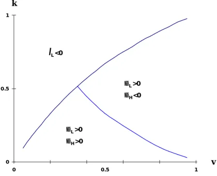
Consider an economy where there are two equally sized groups of workers, low-ability workers with wage wL, and high ability workers with wage wH. For simplicity, we normalize the average wage rate w to unity; we thus have wL ≡ −1 k and wH ≡ +1 k, with 0≤ ≤k 1. Substituting this into (30), we can make numerical computations of the utility gains ∆L and ∆H for low- and high-income earners from going from a system with no tax arbitrage to a system where arbitrage is allowed. The results for the case of α =1 in ( , )v k space are shown in Figure 1.
(Figure 1)
We see, first, that one has to take the non-negativity constraint on labor supply seriously. By (27), lA
∗
can be negative for small values of w. We have therefore simply assumed that the parameters are such that labor supply will be positive, the parameter configurations in ( ,v w space not satisfying this being in the upper left part) of Figure 1. For other, admissible parameter configurations, we see that it is easy to
find cases where both high- and low-income earners gain from the introduction of tax arbitrage, i.e., where both ∆H and ∆L are positive.
5. Labor supply in a model with outside assets
It is well known that the assumption of a perfect capital market has strong
implications for the extent of tax arbitrage. In an interesting paper Stiglitz (1983) shows that existing provisions of the capital income tax can be exploited to the utmost by a rational investor with access to a perfect capital market. A well-informed investor may not only avoid all taxes on asset income, but also all taxes on labor income as well. But, as noted by Stiglitz, the fact that governments collect tax revenue seems to suggest that there are limits to the arbitrage process. One obvious explanation is that imperfections in the capital market make it difficult to completely avoid taxation.
In this section we will comment on how asset trade interacts with labor supply decisions when there are imperfections in the capital market. As in the previous section, we model a situation when the only reason for asset trade is the desire to reduce tax burden when marginal tax rates differ across individuals. But we now assume that the tax exempt asset is an outside asset in fixed total supply, and that this asset (which we for simplicity refer to as land) cannot be sold short. We assume that land is productive, in the sense that each land unit produces ρ units of the
consumption good.10 The introduction of land means that there is an additional layer of heterogeneity in the model. Each individual is now identified by the vector ( ,w X ,) which is distributed in two-dimensional space according to the joint cumulative distribution function F w X( , ) , where X is the initial land endowment.
10
We thus maintain the notion of a two-good economy, where individuals derive utility from consumption and leisure. Also, we assume that the production function for the consumption good is linear in its two arguments, labor and land, which implies that the marginal product of each factor is independent of the other factor.
5.1 Partial equilibrium
Asset trade proceeds as follows. At the beginning of the period, individuals exchange land endowments for taxable consumption loans. This exchange takes place at the per unit land price P. For any individual the proceeds from sales/purchases of land can then be written as P(X- X ), where X is the holding of land at the end of the period, when production occurs. Due to the restriction on short sales, X ≥0 . As there can be no net savings in our one-period model, any change in an individual’s land value is matched by a corresponding transaction of the opposite sign in the taxable asset. Specifically, an individual who purchases land in the positive amount of P(X- X ) increases tax deductible debt with the same amount. As before, r is the interest rate on the taxable asset.
The individual maximizes Max u c s t c X r X X w T w r X X X A X A A A A A l l l l , ( , ) . . ~( ) ( ~( )) 1 0 − = − − + − − − ≥ ρ (32)
where ~r =rP. The first-order conditions become
l l l l A A A A A A u c u c w T w r X X : ( , ) ( , ) ( ( ~( )) 2 1 1 1 1 − − = − ′ − − (33) X r T w r X X if X A : ρ− ( − ′( − ~( − ))≤ = > 1 0 0 0 l (34)
The complementary slackness condition implicit in (34) has important implications for the shape of the labor supply function. Individuals who face a binding quantity constraint in the credit market react to different labor supply incentives than those who are at an interior portfolio optimum.
Consider first the case of an interior solution, when (34) holds as an equality. For individuals for which X > 0, tax arbitrage is driven to the point where the after-tax return on the taxable asset equals ρ. For this group of workers, the constraint on short sales is not an issue, and labor supply will be determined in a way that parallels our analysis in section 3. The relevant marginal tax rate is the yield ratio ρ / ~r, which is the same for everyone. It is easy to show that the behavioral functions take the form
lA =lA( / ~, , ~ )ρ r w r X (35)
ρX = X( / ~, , ~ ) ,ρ r w r X (36)
i.e., the tax system is linearized. Compared with the analysis in section 3, the only novelty is that (35) and (36) include an income effect from the initial land endowment.
To derive the labor supply function for workers who are at a corner solution, we simply set X=0 in (33). We then have
lA =lA( , , ~ )τ w r X , (37)
The labor supply functions of individuals who are at a corner solution will be of the same format as those materializing from the standard labor supply model in the
presence of a nonlinear tax system. In particular, the labor supply function will depend on a vector of parameters, τ, summarizing global properties of the tax system.11
Although individuals at corner solutions engage in intra-marginal asset trade, what matters for the form of the labor supply function is the extent of tax arbitrage on the margin.
11
5.2 Market Equilibrium
To characterize the determination of equilibrium asset prices we need to derive the selection criterion that allocates individuals between the arbitrage and no-arbitrage regimes. Consider an individual for which the non-negativity constraint is binding. For this individual we can write (34) as
[
]
ρ τ φ τ ρ
~ ( , , ~ ) ~ ( , , ~ , / ~ )
r − + ′1 T wlA w r X + r X ≡ w r X r <0.
In the limit the equation φτ( , , ~ ,w r X ρ/ ~ )r =0 then gives us the surface in ( ,w X -) space that separates those who are at an interior optimum from those who are at a corner solution. For the particular case of a logarithmic utility function and a tax system with constant residual tax progression, analyzed in the previous section, the separating surface can be given an intuitive interpretation. After straightforward but tedious manipulations, one can show that the separating hyperplane can be written as
w r X v v r v v + = + ⋅ − ~ ~ α ρ β 1 1 1 . (38)
Everybody with a full income w+ r X~ less than the right-hand side of (38) will be in a constrained optimum, while everybody with a full income that is greater than or equal to the right-hand side will be in an unconstrained optimum. Inherently poor
individuals will face a binding credit constraint and a nonlinear tax system, and they will supply labor according to (37). Inherently rich individuals will face a perfect capital market and a linearized tax system, and they will supply labor according to (35).
We can now integrate the demand function (36) over all unconstrained
individuals to obtain aggregate land demand. In equilibrium, this has to be equal to the total quantity of land available (which we for simplicity set equal to unity):
X( / ~,r w, X dF w X) ( , ) (.) ρ ρ ρ φ
∫
≥ = ⋅ 0 1. (39)This equilibrium condition allows us to solve for the endogenous variable ~r , or rather for the price of land, since ~r ≡rP.12 Finally, we should note that (39) gives us the equilibrium price for any tax system τ . Since we constrain ourselves to purely redistributive systems, we require τ to be such that the government budget is balanced.
5.3 Some implications for empirical estimation of labor supply response
In one form or another, the static labor supply function (37) has been at the center of attraction in a large number of microeconometric studies that try to estimate how labor supply reacts to changes in economic incentives. Much of this literature has been preoccupied with the design of econometric techniques capable of dealing with
nonlinear tax systems. In this process, the typical individual is modeled as maximizing utility with respect to work hours, subject to a nonlinear budget constraint that treats reported capital income as an exogenous -- positive or negative -- constant. Our analysis suggests that this procedure creates two main problems.
First, there is the issue of self-selectivity. Based on initial asset endowments and productivity in the labor market, individuals choose between two labor supply functions. For arbitrageurs there is no way of separating asset choice from labor supply, the formal bracket schedule provides no information about marginal work incentives, and equation (35) applies. For individuals who face a binding constraint in the asset market, the formal bracket schedule conveys all the information that is needed about marginal work incentives, and equation (37) applies. Econometric
studies that build on the assumption that the labor supply function looks the same for all individuals will come up with biased estimates.
Second, to repeat a point made in a previous section, there is the issue of measurement error in net capital income. The prime evidence about labor supply in Sweden, and in many other countries, stems from studies that rely on data from individuals’ tax returns. But the essence of tax arbitrage is that people invest their wealth in ways that are imperfectly measured or registered by the tax authorities. The resulting error in the measurement of net capital income will typically be correlated with the gross wage. The income tax returns of high-wage individuals will to a much greater extent than the income tax returns of low-wage individuals understate true capital income. As a consequence, there will be a downward bias in the estimate of the gross wage coefficient. What the econometrician interprets as evidence of a backward bending labor supply function may in reality reflect the influence of unobservable asset income.
12
6. Concluding remarks
A critic is certainly justified in arguing that our analysis rests on a number of strong assumptions. First, tax avoidance amounts to more than paper transactions in asset markets -- many avoidance strategies involve activities that have a direct effect on utility (e.g. purchasing a leveraged house). Second, unlimited trade in inside assets, which was a key assumption in section 3, is hardly an admissible option for the vast majority of households. Third, our analysis of capital market imperfections in section 5 is specific rather than general. Fourth, our single-period model does not account for the fact that there is an intertemporal dimension to many common tax arbitrage strategies. Developing models that relax these and other restrictive assumptions certainly seem like a worthwhile exercise.
Even though one must be aware that our results have been derived within a simple framework, we believe that our analysis sheds light on a number of positive and normative issues concerning modern tax systems.
First, what makes people work, given the very high marginal tax rates that can be observed for some countries (e.g., Sweden) during some periods? A traditional answer has been that labor supply is rather inelastic, a view which has been intimately related to some recent attempts to estimate labor supply functions and deadweight burdens. Our proposed answer is different. With the tax avoidance technologies that became increasingly available during the 1980s, people that cared very much about incentives need not pay those high marginal rates. The effective tax schedules were quite different from the official ones.
Second, how come so many countries turned their tax systems into simple, linear ones during the 1980s and 1990s? Our suggested answer is that during this period, credit markets became increasingly well-functioning. Thus the effective tax
schedules became more and more linear, and the various reforms that took place can be seen as a simple recognition of this fact.13
Third, are sophisticated non-linear optimal tax schedules in the spirit of Mirrlees (1971) really relevant? In the presence of unlimited tax arbitrage such nonlinear second-best tax schedules clearly are not attainable. Regardless of the ambitions underlying the official, non-linear schedule, the raw force of profit-seeking tend to linearize the effective tax schedule. A government maximizing social welfare may have to settle for a third-best solution, which involves finding an optimal linear income tax.
Fourth, models that allow for tax arbitrage and asset trade may have important implications for empirical analysis of behavioural response. As discussed in the previous section, studies that ignore the effect of tax arbitrage and asset trade on labor supply incentives are likely to come up with biased estimates of important supply elasticities. Econometric work taking various tax avoidance technologies into account is still in its infancy.
Fifth, there is the important question on the correct way of measuring the deadweight burden of the income tax. Feldstein (1995b) argues that in the presence of tax avoidance, the sensitivity of taxable income to tax changes is a proper indication of the deadweight burden, and that models that account for tax avoidance will produce calculations of deadweight losses that are many times larger than those implied by standard Harberger-calculations. These claims have however not yet been analyzed for a wide class of models, and thus their generality is disputed. Our framework can be used for a thorough investigation of the validity of Feldstein´s claim for a class of
13 For some interesting discussion and analysis of the reasons for tax reforms in the Nordic countries, see Sørensen (1994) and Nielsen and Sørensen (1997).
models where tax avoidance occurs in the form of trade in well-functioning asset markets. As we demonstrated in section 4, it is indeed easy to construct examples where asset trade reduces the efficiency cost of income taxation.
Sixth, from a public choice perspective tax arbitrage and a highly progressive tax system can be viewed as an ingenious way of reconciling incompatible political ambitions. High marginal tax rates convey the message that politicians care about the less well off, while a generous attitude towards tax avoidance prevents the very same tax system from destroying the incentives of the rich and the highly educated. The political economy of tax design seems like an important research topic for the future.
References
Ackum Agell, S. and C. Meghir, 1995, Male labour supply in Sweden: Are incentives important?, Swedish Economic Policy Review 2, 391-418.
Agell, J. and P.-A. Edin, 1990, Marginal taxes and the asset portfolios of Swedish households, Scandinavian Journal of Economics 92, 47-64.
Agell, J., P. Englund and J. Södersten, 1996, Tax reform of the century – the Swedish experiment, National Tax Journal 49, 643-664.
Agell, J. and M. Persson, 1990, Tax arbitrage and the redistributive properties of progressive income taxation, Economics Letters 34, 357-361.
Allingham, M.G. and A. Sandmo, 1972, Income tax evasion: A theoretical analysis, Journal of Public Economics 1, 323-338.
Aronsson, T. and M. Palme, 1995, A decade of tax and benefit reforms in Sweden – effects on labor supply, welfare and inequality, Tax Reform Evaluation Report No. 2. Stockholm: National Institute of Economic Research. Auerbach, A. and J. Slemrod, 1997, The economic effects of the tax reform act of
1986, Journal of Economic Literature 35, forthcoming.
Bergstrom, T. and S. Blomquist, 1993, The political economy of subsidized day care, European Journal of Political Economy 12, 443-458.
Blomquist, S. and U. Hansson-Brusewitz, 1990, The effects of taxes on male and female labor supply in Sweden, Journal of Human Resources 25, 317-357. Blomquist, S., 1996, Estimation methods for male labor supply functions. How to take
account of nonlinear taxes, Journal of Econometrics 70, 383-405.
Cowell, F. A., 1990, Cheating the government: the economics of evasion, The MIT Press, Cambridge, MA.
Feldstein, M., 1995a, The effect of marginal tax rates on taxable income: A panel study of the 1986 tax reform act, Journal of Political Economy 103, 551-572. Feldstein, M., 1995b, Tax avoidance and the deadweight loss of the income tax,
Working paper no. 5055, National Bureau of Economic Research, Cambridge, MA.
Gottschalk, P. and T. Smeeding, 1997, Cross-national comparisons of earnings and income inequality, Journal of Economic Literature 35, 633-687.
Hausman, J.A., 1981, Labor supply, in: H.J. Aaron and J.A. Pechman, eds., How taxes affect economic behavior, Brookings Institution, Washington, DC.
Jakobsson, U., 1976, On the measurement of the degree of progression, Journal of Public Economics 5, 161-168.
Lindbeck, A., 1995, Hazardous welfare-state dynamics, American Economic Review 85 (Papers and Proceedings), 9-15.
Lindencrona, G., 1993, The taxation of financial capital and the prevention of tax avoidance. In Tax reform in the Nordic countries, 1973-1993 Jubilee publication of the Nordic council for tax research. Uppsala: Iustus.
MaCurdy, T.E., D. Green and H. Paarsch, 1990, Assessing empirical approaches for analyzing taxes and labor supply, Journal of Human Resources 25, 415-490. Malmer, H. and A. Persson, 1994, Skattereformens effekter på skattesystemets
driftskostnader, skatteplanering och skattefusk (The effects of the tax reform on compliance costs, tax planning, and tax fraud). In Århundradets
skattereform (Tax reform of the century), edited by H. Malmer, A. Persson and Å. Tengblad. Stockholm: Fritzes.
Mayshar, J., 1991, Taxation with costly administration, Scandinavian Journal of Economics 93, 75-88.
Miller, M., 1977, Debt and taxes, Journal of Finance 32, 261-275.
Mirrlees, J., 1971, An exploration in the theory of optimum income taxation, Review of Economic Studies 38, 175-208.
Myrdal, G., 1978, Dags för ett nytt skattesystem (Time for a new tax system), Ekonomisk Debatt 6, 493-506.
Nielsen, S. B. and P. B. Sørensen, 1997, On the optimality of the Nordic system of dual income taxation, Journal of Public Economics 63, 311-329.
Persson, M., 1995, Why are taxes so high in egalitarian societies?, Scandinavian Journal of Economics 97, 569-580.
Sandmo, A., 1981, Income tax evasion, labour supply, and the equity-efficiency tradeoff, Journal of Public Economics 16, 265-288.
Sandmo, A., 1991, Economists and the welfare state, European Economic Review 35, 213-239.
Slemrod, J., 1992, Do taxes matter? Lesson from the 1980s, American Economic Review 85 (Papers and Proceedings), 250-256.
Slemrod, J., 1994, A general model of the behavioural response to taxation, mimeo. Sørensen, P. B., 1994, From the global income tax to the dual income tax: Recent tax
reforms in the Nordic countries, International Tax and Public Finance 1, 57-79.
Stiglitz, J., 1983, Some aspects of the taxation of capital gains, Journal of Public Economics 21, 257-294.
Stiglitz, J., 1985, The general theory of tax avoidance, National Tax Journal 38, 325-337.
Summers, L., J. Gruber, and R. Vergara, 1993, Taxation and the structure of labor markets: The case of corporatism, Quarterly Journal of Economics 108, 385-411.