Mälardalen University Press Licentiate Theses No. 123
CONTROLLED MANIPULATION OF MICROPARTICLES
UTILIZING MAGNETIC AND DIELECTROPHORETIC FORCES
LarsErik Johansson 2010
Copyright © LarsErik Johansson, 2010 ISBN 978-91-86135-93-5
ISSN 1651-9256
Mälardalen University Press Licentiate Theses No. 123
CONTROLLED MANIPULATION OF MICROPARTICLES UTILIZING MAGNETIC AND DIELECTROPHORETIC FORCES
LarsErik Johansson
Akademisk uppsats
som för avläggande av teknologie licentiatexamen i bioteknik/kemiteknik vid Akademin för hållbar samhälls- och teknikutveckling kommer att
offentligen försvaras måndagen den 15 november, 2010, 10.00 i Selandersalen, Kv. Verktyget, Mälardalens högskola, Eskilstuna.
Opponent: Professor Leif Nyholm, Uppsala Universitet, Ångström Laboratoriet, Institutionen för materialkemi.
Mälardalens Högskola
Abstract
This thesis presents some experimental work in the area of manipulation of microparticles. Manipulation of both magnetic and non magnetic beads as well as microorganisms are addressed. The work on magnetic bead manipulation is focused on controlled transport and release, on a micrometer level, of proteins bound to the bead surface. Experimental results for protein transport and release using a method based on magnetization/demagnetization of micron-sized magnetic elements patterned on a modified chip-surface are presented. Special attention has been placed on minimizing bead-surface interactions since sticking problems have shown to be of major importance when protein-coated beads are used. The work with non-magnetic microparticles is focused on the dielectrophoretic manipulation of microorganisms. Preliminary experimental results for trapping and spatial separation of bacteria, yeast and non-magnetic beads are presented. The overall goal was to investigate the use of dielectrophoresis for the separation of sub-populations of bacteria differing in, for example, protein content. This was, however, not possible to demonstrate using our methods. Within the non-magnetic microparticle work, a method for determining the conductivity of bacteria in bulk was also developed. The method is based on the continuous lowering of medium conductivity of a bacterial suspension while monitoring the medium and suspension conductivities.
To my family
…closing the tweezers without moving the bacteria out of the way
required patience…
List of papers
This thesis is based on the following papers:
I “A magnetic microchip for controlled transport of attomole levels of proteins”
LarsErik Johansson, Klas Gunnarsson, Stojanka Bijelovic, Kristofer Eriksson, Alessandro Surpi, Emmanuelle Göthelid, Peter Svedlindh and Sven Oscarsson, Lab Chip (2010) 10: 654 - 661.
II “Determination of Conductivity of Bacteria by Using Cross-Flow Filtration”
LarsErik Johansson, Fredrik Aldaeus, Gunnar Jonsson, Sven Hamp and Johan Roeraade, Biotechnology Letters (2006) 28: 601-603. III “A study of biological particles in Bio-Mems devices using
dielectrophoresis”
Mats Jönsson, Fredrik Aldaeus, Lars-Erik Johansson, Ulf Lindberg, Johan Roeraade, Ylva Bäcklund, Sven Hamp, Gunnar Jonsson. Proceedings of the Fifth Micro Structure Workshop (MSW) 2004, Ystads Saltsjöbad the 30-31 March 2004.
IV “A Simple Open Micro System for Dielectrophoresis and Impedance Measurements”
Mats Jönsson, Fredrik Aldaeus, LarsErik Johansson, Ulf Lindberg, Johan Roeraade, Sven Hamp, Gunnar Jonsson
Author contribution Paper I.
Major part of bead-transportation experiments and chemical modifications of bead- and chip surfaces. Significant part of planning, evaluation and writing.
Paper II.
Major part of experimental work. Significant part of planning, evaluation and writing.
Paper III
Major part of experimental work regarding dielectrophoresis. Part of planning, evaluation and writing.
Paper IV
Significant part of experimental work regarding dielectrophoresis. Part of planning, evaluation and writing.
The work has also been presented at the following conferences:
P1 “Transport of protein-covered magnetic beads at modified chip-surfaces”
LarsErik Johansson, Klas Gunnarsson, Stojanka Bijelovic, Kristofer Eriksson, Emmanuelle Göthelid, Peter Svedlindh and Sven
Oscarsson
Poster at ESF-EMBO Symposium Biomagnetism and Magnetic Biosystems Based on Molecular Recognition Processes 2007, St. Feliu de Guixols, Spain, 22-27 August 2007.
P2 “Programmable Motion and Separation of Single Magnetic Particles on Patterned Magnetic Surfaces”
LarsErik Johansson, Klas Gunnarsson, Erika Ledung, Sven Oscarsson, Peter Svedlindh.
Poster at Sixth Micro Structure Workshop (MSW) 2006, Västerås, 9-10 May 2006.
P3 “Dielectric Characterisation of Microorganisms”
Sven Hamp, LarsErik Johansson, Gunnar Jonsson, Fredrik Aldaeus, Mats Jönsson.
Poster at Sixth Micro Structure Workshop (MSW) 2006, Västerås, 9-10 May 2006.
P4 “Escherichia coli behavior in an open dielectrophoretic microsystem”
Fredrik Aldaeus, Lars-Erik Johansson, Mats Jönsson, Gunnar Jonsson, Ulf Lindberg, Johan Roeraade, Sven Hamp.
Poster at 4th Workshop of Nanochemistry and Nanobiotechnology. Saltsjöbaden 2004.
Contents
Introduction...1
1.Manipulation of micro-particles...3
Manipulation based on magnetism...3
Manipulation based on dielectrophoresis...5
Manipulation based on other forces...7
2.Surface forces and Brownian motion...10
Surface forces...10
Brownian motion...21
3.Dielectrophoretic and magnetic forces...22
Dielectrophoresis...22
Magnetism...28
4.Methods...33
Electric conductivity measurement...33
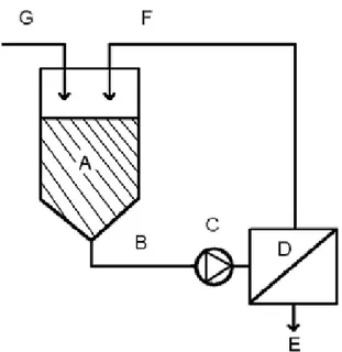
Cross-flow filtration...35
Light and fluorescence microscopy...37
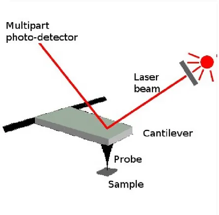
Scanning probe microscopy...38
UV-VIS Spectrophotometry...41
Surface modifications for reducing protein-surface interactions...42
Physical methods for surface modification...43
Protein coupling chemistry...45
5.Summary and discussion of papers...47
Paper I...47
Paper II...51
Paper III...53
Paper IV...57
Svensk populärvetenskaplig sammanfattning...60
Acknowledgments...61
Abbreviations
AFM Atomic Force Microscopy
DACS Dielectrophoresis Activated Cell-Sorter DEP Dielectrophoresis
DNA Deoxyribose Nucleic Acid EDL Electric Double Layer
FACS Fluorescence Activated Cell-Sorter HSA Human Serum Albumine
MEMS Micro Electromechanical System MFM Magnetic Force Microscopy µTAS Micro Total Analysis System PBS Phosphate Buffered Saline PDMS Polydimethylsiloxane PEO Polyethylene oxide
SPM Scanning Probe Microscopy STM Scanning Tunneling Microscopy SDS Sodium Dodecyl Sulphate UV Ultra violet
SDS-PAGE Sodium Dodecyl Sulphate Polyacrylamide Gel Electrophoresis XPS x-ray photoelectron spectroscopy
Introduction
The aim of this thesis is to present experimental results of some methods for the manipulation of microparticles. The term particles can stand for many things: for a particle physicist it can mean elementary particles whereas for a physical chemist it can mean nanoparticles which have dimensions below about 500 nm (the lower limit is not very well defined, but atoms and small molecules are not considered nanoparticles). Particles in the size range 0.5 – 100 µm are often referred to as microparticles and are, as the title indicates, an important component of this thesis. In the collective term microparticles, we can include cells, bacteria, large viruses, clay particles and dust to mention a few. Microparticles can be highly complex, such as a cell, or very simple, such as a silica particle, and a spectrum of complexities in between. Cells, bacteria and viruses are often referred to as bioparticles in the literature, especially in applied physics and microsystem technology.
In our everyday life, we often encounter microparticles, e.g. when brushing our teeth. Titanium dioxide (E171) microparticles make toothpaste look appealing due to its optical properties and are a part of the polishing process. Microparticles in foods are used for example as nutrient delivery vehicles to protect, for example, a sensitive vitamin in a food and release it in some part of the gastrointestinal system (Chen and Subirade, 2006). Another everyday example is glass microparticles that are used in road markers to improve light reflection (Swarco Vestglas GmbH). In pharmaceutical applications, microparticles can be used to control drug release by encapsulating the drug in the microparticle (microcapsules) or dispersing the drug through the matrix of the microparticle (microspheres) (Lasalle and Ferreira, 2007). The use of microparticles in bioanalysis is demonstrated in several papers, for example bar-coded particles, where each particle carries an individual readable code which enables immediate visual identification of that particles specific chemical functionalization (Pregibon, Toner and Doyle, 2007). In separation science, microparticles have been used for decades to build up chromatographic media (Porath and Flodin, 1959). By fine-tuning the size, matrix and surface chemistry of the particles it is possible to make chromatographic media for ion-exchange, reversed-phase, affinity, size-exclusion etc. Solid phase synthesis is another important area where molecules are synthesized on a microparticle surface. By having the
by-products washed away with the product held in place. Today, chemical companies provide solid phase resins with a wide variety of surface functionalization. When the Norwegian researcher John Ugelstad developed monodispersed polymer microbeads and incorporated magnetic material in microbeads in the 1970s to 1980s, this led to a new means of separation in biotechnological applications. Since most biomaterial does not interact with magnetic fields, it became easy to selectively manipulate beads with a magnetic field without disturbing the rest of the material. Applications of magnetic beads include e.g. separation of whole cells, proteins and bacteria from complex samples (Vartdahl et al., 1986).
Manipulation of microparticles relative to their environment has been demonstrated by use of several techniques such as physical trapping, transportation, separation or rotation of the particle. Some methods for these types of manipulation are reviewed in this thesis, with some basic theory in a separate chapter. Due to their high surface/volume ratio, surface interactions can be a problem with micro- and nanoparticles, and thus a chapter on the basics of surface forces has also been included.
Paper I describes a novel system for the transport and release of proteins bound to magnetic beads performed on a chip-surface. Paper II describes a novel method for determining the conductivity of bacteria in bulk. Paper III and IV describe some preliminary studies of dielectrophoresis as a tool for manipulation of bacteria, yeast and beads.
1. Manipulation of micro-particles.
Manipulation based on magnetism
Magnetism-based methods for manipulation of (magnetic) beads range from mass-manipulation down to manipulation of single beads. For micro-scale manipulation of magnetic beads different strategies have been presented. A so-called unit operation of a magnetic bead-based micro-system is trapping of the magnetic beads. Smistrup et al. (2006) used micro-electromagnets placed below a flow-channel to capture, and subsequently release, a group of 1.1 µm diameter magnetic beads within the channel. Choi et al. (2000) also used micro-electromagnets to capture magnetic beads (1 µm diameter) from a fluid flow on a chip surface. Incorporated in their device was a sensing coil, which measured the inductance change as magnetic beads were trapped on the surface. A similar strategy was used by Ramadan et al. (2006ab) who used ferromagnetic pillars, magnetized by micro-electromagnets, to capture groups of magnetic beads (1-5 µm diameter) in a microfluidic device. The purpose of the pillars was to focus the magnetic field from the coils and locally create a high magnetic field gradient in order to enhance the trapping of beads. The magnetized pillar was situated outside of the flow channel containing the beads. Furthermore, a sensing coil was located close to the coil generating the trapping field. As a result of beads accumulating on top of the pillar, the inductance in the sensing coil changed and the presence of beads could thus be detected. Yellen and Friedman (2004) assembled patterns of magnetic beads in micro-wells on a chip by individually addressing magnetic elements with one end positioned within the well. A specific element can have its magnetization direction altered by selectively heating that element with a laser in the presence of an in-plane external magnetic field. By heating the element, it is can more easily have its magnetization direction altered by the external magnetic field than the non-heated elements, which are unaffected by the in-plane field. When the in-in-plane field is switched off, beads can be positioned in the well by binding to the element which have had its magnetization altered. The attraction of beads to the elements is due to a weak out-of-plane field which is always present in the experiment, and which vertical direction determines the attraction/repelling of beads to the elements. The “active”
well is filled with beads, the element is switched off by changing back the magnetization direction. The beads remain within the well by ensuring to keep the vertical field weak enough to hinder the beads from being fully repelled. The presence of beads in the well also blocks it from contamination of other beads. Due to this, the chip can be rinsed and other elements can be switched on and other bead types can be bound to these.
Another type of unit operation of a magnetic bead-based micro-system is controlled movement of the magnetic beads relative to the environment. Lee, Purdon and Westervelt (2004) used microelectromagnets to demonstrate capture of single magnetic beads (2.1 µm diameter), yeast cells bound to a single magnetic bead (2.8 µm diameter) and magnetotactic bacteria (Magnetospirillum magnetotacticum). In the paper, the authors also demonstrated transportation of magnetic beads over a chip surface by the use of a matrix of microelectromagnets. In the latter experiment the beads were not controlled one-by-one, but as a small group. Deng et al. (2001) used a system of current-carrying micro-circuits to create localized magnetic field maxima on a micro-chip. By changing the location of the field maxima, groups of magnetic beads (4.5 µm diameter) were moved along the circuits. The field maxima were changed by altering the current direction in the circuits. Janssen, van Ijzendoorn and Prins (2008) moved magnetic beads (1 – 2.8 µm diameter) between two current carrying wires on a chip. The beads were moved between the two wires by alternatively running a current through the two wires. The beads are magnetized by the field due to the wires and attracted by the field gradient. In the paper, the author also demonstrated a magnetic sensor, positioned in-between the two wires, which was capable of detecting the position of a single magnetic bead between the wires. Gunnarsson et al. (2005) used a line of soft magnetic elements in conjunction with a rotating magnetic field to transport single magnetic beads on a silicon surface. A bead follows the rim of an element synchronously with the rotation of the field until it reaches a position where it due to geometric reasons is more strongly attracted by a neighboring element and thus makes a jump to that element. In the same paper, a sorting mechanism is demonstrated, which enables a magnetic bead to shift into a side-track by reversing the rotation of the magnetic field. In this thesis, utilizing the method of Gunnarsson and co-workers, a novel method for controlled transport and release of proteins bound to magnetic beads is presented (paper I).
Manipulation based on dielectrophoresis
Dielectrophoresis was discovered in the 1950s by Herbert Pohl (Pohl, 1951) and is today used for micro- and nanoscale manipulation of various micro- and nanosized objects, of both synthetic and biological origin. A separate chapter describing some basics of dielectrophoresis is included in this thesis. Dielectrophoresis benefits from micro-fabrication technology, since quite high field strengths and gradients, two of the factors that determine the dielectrophoretic force, are achievable with low voltages when micro-electrode structures are used (Hughes, 2003). Low voltage demands (typically a few volts) provide a great advantage when building battery-driven, portable devices.
With dielectrophoresis it is possible to trap, or capture, objects ranging in size from a few nanometers to tenths of micrometer. It is also possible to use dielectrophoresis to create patterns of small objects on the surface or to move them around. Beck et al. (2008) used dielectrophoresis to trap single bacterial spores between two electrodes in order to perform electrical characterization of the spores. The authors were able to discriminate between spores of several Bacillus species by their current response at 10 kHz. The authors related the differences in electric response to differences in the surface chemistry of the spores, since some of the discriminated species were of a comparable size. Frénéa et al. (2003) used an electrode array to position mammalian cells in wells fabricated on a chip by placing the electrodes in a pattern so that the wells coincided with low-field regions where the cells experienced negative dielectrophoresis. Also demonstrated in that paper was the positioning of beads (3 µm diameter) in an electrode defined pattern. Alp, Stephens and Markx (2002) positioned bacteria and mammalian cells in a pattern on micro electrodes by utilizing positive dielectrophoresis. Layers consisting of up to 3 species vertically stacked or placed adjacent were constructed. Further, an artificial biofilm was constructed by polymerizing acrylamide on top of the structured species. Other examples are trapping of viruses (Morgan and Green, 1997 ; Green, Morgan and Milner, 1997) and sub-micrometer beads (Green and Morgan 1999). It is also possible to utilize dielectrophoresis to trap DNA and proteins at micro-electrodes (Washizu et al., 1994; Bakewell et al., 1998). Kawabata and Washizu (2001) demonstrated direct trapping of DNA and proteins at micro electrodes placed in a micro channel. Also demonstrated in
lambda-DNA (48500 base-pairs): The larger DNA-molecule is more readily attracted to the electrodes, since the dielectrophoretic force is size-dependent (see chapter 3). Other experiments in the paper use a DEP-enhancer, i.e. they selectively bind the target to a bead or molecule which can be manipulated by dielectrophoretic forces. Both the (obvious) use of a polystyrene bead and the use of lambda-DNA as the enhancer is demonstrated in the paper. Stretching of DNA between two electrodes has been demonstrated by Namasivayam et al. (2002). The authors connected one end of the DNA molecule to the edge of one of a pair of pointed micro-electrodes by chemical means. An AC-electric field was applied, thus making the DNA line up between the electrodes in a controlled way.
Dielectrophoresis can also be used for controlled movement of cells. Suehiro and Pethig (1998) manipulated plant protoplasts (30-50 µm diameter) in a controlled way in 2D by using a 3D grid of individually wired microelectrodes. In their system the cell is moved within the grid with the aid of locally induced negative and positive dielectrophoresis zones.
Dielectrophoresis-based separations have been studied for some decades and several types of separation have been demonstrated. In a paper by Markx and Pethig (1995), a system for continuous separation of cells is described. Live and dead yeast cells were separated based on differences in their dielectrophoretic response in combination with a fluid drag-force. The live cells were held tighter towards an electrode pattern than the dead cells and could therefore resist the fluid drag. A system of pumps and valves in combination with switching the field on and off made the system work in continuous mode. In another work by Markx, Dyda and Pethig (1996), different types of bacteria were separated based on their dielectrophoretic response. By varying the conductivity of the suspending medium they were able to selectively release one type of bacteria from an electrode pattern whereas the other type was still held in place. Recently, Pommer et al. (2008) demonstrated separation of platelets from diluted whole blood in a dielectrophoretic activated cell-sorter (DACS). The basis of the DACS described in the paper is the dielectrophoretic deflection of cells (larger than platelets) in a stream of the blood sample into a waste-stream.
Techniques related to dielectrophoresis are traveling wave dielectrophoresis and electrorotation. Traveling wave dielectrophoresis and electrorotation are, in turn, closely related to each other in the sense that both make use of a phase-shifted field to induce a torque on the particle to either transport it
along a lane of electrodes or rotate it on a spot, surrounded by the electrodes. The books by Morgan and Green (2003) or Hughes (2003) are strongly recommended for the interested reader; however the theory of the subject is outside the scope of this thesis.
In this thesis, a novel method for determining the conductivity of bacteria in bulk is described (paper II). Also some preliminary work with dielectrophoretic manipulation of bacteria, yeast and beads are described (paper III and IV).
Manipulation based on other forces
Optical tweezers or optical traps exploit the fact that light exerts force on matter. Dielectric particles, such as uniform beads or bacterial cells, are attracted to and trapped near the waist of a laser beam that has been focused through a microscope objective. It is a so called field gradient technique, which also includes dielectrophoretic and magnetic tweezers.
When the particle is out of focus of the beam, it is exposed to a force pulling it back to focus (if the particle is transparent) or away from focus (if the particle is opaque). Furthermore, the particle will interact with the light-gradient in exactly the same way as in dielectrophoresis, causing it to move away from or towards high field gradients (Hughes, 2003). The forces acting on the particle are dependent on the refractive index, size and shape of the object as well as the intensity and wavelength of the beam. The refractive index is related to the dielectric constant (Nordling and Österman, 2004, p. 264).
Optical tweezers were invented during the 1970s by Arthur Ashkin (Ashkin, 1997) and have found great use in e.g. cell manipulation. The first reports on manipulation of particles in micron size were in 1986 by Ashkins group (Ashkin et al., 1986). In 1987 the same group reported trapping of micro-organisms such as Escherichia coli and Saccharomyces cerevisiae (Ashkin, Dziedzic and Yamane, 1987). In Lab-On-A-Chip applications, the technique is gaining interest. Enger et al. (2004) used optical tweezers to move E. coli cells between different reservoirs in a micro chip. In the same publication, optical tweezers were used to trap a single S. cerevisiae cell in a flow of E. coli and S. cerevisiae and moved it into a side channel on the chip.
Optical tweezers have also been used in single molecule studies, e.g. stretching of DNA (Smith, Cui and Bustamente, 1996) and for studies of
protein properties on the molecular level (Tskhovrebova, Sleep and Simmons, 1997; Svoboda et al. 1993).
Ultrasound can be used to trap and position particles. Sound is basically a series of compressions and rarefactions of matter and its interaction with particles is depending on particle size, density and compressibility.
The group of Laurell used an ultrasonic standing wave (a wave that is “fixed” in its position in space) to separate red blood cells from lipids on a micro-chip (Nilsson et al., 2004; Petersson et al., 2005). The red blood cells were focused in the center of a micro-channel, where a pressure node was situated, whereas the lipids were pushed to the walls, where the pressure anti-nodes were situated.
Another work by the same group reports the capture of micro beads in a flow channel (Lilliehorn et al., 2005). Polystyrene beads (about 7 µm diameter) were captured in clusters on top of an ultrasonic transducer mounted in a flow channel.
Mechanical methods for manipulation are methods such as micromechanical tweezers, micro fluidic and SPM-techniques. Piezo-driven mechanical clamps mounted on a micro-manipulator were used by Jericho et al. (2004) to pick up and move Staphylococcus aureus, Escherichia coli and 1.1 µm latex beads on a glass slide. A commercial micro-manipulator with a stepping motor-controlled robotic arm onto which clamps, pipettes or probes can be mounted was used by Jericho´s group. On the molecular and nanometer scale, scanning probe microscopy (SPM) has been used to manipulate single molecules e.g. to stretch molecules (Rief et al., 1997 ; Marszalek et al. 1998) and to position nanoparticles (30 nm size) on a surface (Junno et al., 1995).
Fluid mechanical manipulating methods are often used in the fluorescence activated cell-sorter (FACS). The FACS is in principle a flow cytometer designed to identify (by fluorescence) and sort out specific cells from a fluid stream by controlling the flow direction. Efforts have been made to make the FACS an on-chip method for use in miniaturized diagnostic devices. Wolff et al. (2003) presented an on-chip FACS capable of sorting out fluorescent beads from a mixture of fluorescent beads and red blood cells. By opening a high-speed valve on the side-channel when a fluorescent bead passed a detector, the fluid flow (and the bead) could be directed into that channel. In the same paper, the authors also showed a prototype capable of sorting two populations of yeast cells, one containing green fluorescent protein (GFP)
and one normal. The population containing GFP were sorted to an on-chip cultivation chamber by the valve switching method described above.
2. Surface forces and Brownian motion.
Surface forces
In the systems investigated in this work a very intricate and interesting situation with forces acting between micro-particles (including beads, bacteria and cells) and the chip as well as between the particles themselves could be foreseen. The two main forces counteracting each other are the magnetic and electric forces which are the driving forces for transportation of particles and the “sticking forces” which will act against transportation. As long as the transportation of particles goes on, friction forces (particle-fluid and particle-surface) will also appear. All those forces involved in the techniques described in this thesis have not been experimentally determined since that is beyond the scope of this investigation. On the other hand, many references to other researchers work concerning different techniques for manipulation of micro-particles have been included and in most of these references surface forces have, at the most, been briefly addressed. Nevertheless, consideration of these forces is of crucial importance for this work, especially for the transport of proteins on beads, and thus a summary of most of the general existing knowledge of the forces involved at macromolecule/surface interfaces follows below (Israelachvili, 1985; Atkins, 2000; Norde, 2003).
Intermolecular forces
Intermolecular forces are effective at distances up to about 1 nm. As a comparison, a water molecule is about 0.14 nm in diameter, whereas a 30kD globular protein is about 7 nm in diameter. The forces discussed below are therefore considered short-range as they occur close to molecular contact. Ion-ion interaction
The interaction energy, w, between two charges, Q1 and Q2, a distance r apart is given by Coulombs law,
r
Q
Q
r
w
1
4
)
(
0 2 1⋅
⋅
⋅
⋅
⋅
=
ε
ε
π
where ε is the dielectric constant of the medium between the charges. It follows from the equation that the interaction energy decreases with the inverse of the distance between the charges and with increased dielectric constant of the medium between the charges. Polar solvent molecules such as water (ε =80) tend to orient around ions, which causes a decrease of the ion-ion interaction energy since some of the available energy is needed to keep the solvent molecules oriented. In addition, ions are also surrounded by nearby oppositely charged ions which screen the charge. These effects make the ion-ion interaction quite short range.
Hydrogen bonding
If a hydrogen atom is bond to an electronegative atom, it tends to be polarized and possess a partial positive charge. The partially charged hydrogen can interact with other electronegative atoms situated on nearby molecules or within the same molecule. The hydrogen bond between two molecular groups, E1–H and E2, is generally described as
E1–H- - -E2
where E1 and E2 are two electronegative atoms and the hydrogen bond is present between the hydrogen (which is covalently bond to E1) and E2. Examples of molecules capable of forming hydrogen bonds are water, DNA and proteins. In bulk water, each water molecule can interact with four other water molecules and thus form a three-dimensional network. The basic building block in the network is an oxygen atom surrounded by four hydrogen atoms, two covalently bond to the oxygen, two bound via hydrogen bonding. There is a constant reorganization of hydrogen bonds in aqueous solutions.
Hydrophobic interaction
If a molecule incapable of forming hydrogen bonds is introduced in water, the water molecules will structure themselves around the molecule. This structuring lowers the entropy of the water molecules, and is thus thermodynamically unfavorable. If more of these molecules are introduced, they tend to aggregate to minimize the exposed surface towards water and thus minimizing the amount of structured water. This entropy-based
interaction between molecules in water is known as the hydrophobic interaction.
Ion-dipole interaction
A dipole consists of two opposite charges separated by a distance. If placed close together with a charge (Q), a fixed dipole will interact by both a repulsive and an attractive force since the dipole possesses two different charges. The geometrical position of the dipole relative to the charge as well as the dipole moment (u) will influence the interaction energy, w, as described by the (approximate) expression
2 0
)
cos(
4
)
,
(
r
u
Q
r
w
θ
ε
ε
π
θ
⋅
⋅
⋅
⋅
⋅
−
=
where cos(θ) is the angle between the field line from the charge and the direction of the dipole. The direction of the dipole is (by definition) from the negative to the positive end, whereas the electric field line is directed (by definition) from positive to negative potential. From this follows the minus sign (attractive force) at angles between 0-90° and 270-360°. Attractive force means that the dipole has its oppositely charged end closest to the charge of interest. The above expression is valid when the dipole is small compared to the distance from the charge.
If the dipole can rotate freely, the interaction energy, w, will also be dependent on thermal energy according to
4 2 0
6
1
4
)
(
r
T
k
u
Q
r
w
⋅
⋅
⋅
⋅
⋅
⋅
⋅
⋅
−
=
ε
ε
π
with the notation as above, k being the Boltzmann constant and T being the absolute temperature. As in the previous expression, the dipole must be small compared to the distance from the charge for the expression to be valid.
Dipole-dipole interaction
If two nearby dipoles, u1 and u2, are fixed at an arbitrary orientation in space, the interaction energy, w, between the two dipoles will be given by
3 0 2 1 4 ) ( r const u u r w ⋅ ⋅ ⋅ ⋅ ⋅ − = ε ε π
where the constant, const, is dependent on the relative orientation of the dipoles in space: Consider one of the dipoles restricted to rotation (θ1) around its center in a plane, then place the other dipole with its center fixed in the same plane, at the distance r, and allow that dipole to rotate both in the plane (θ2) and out of the plane (φ). This arrangement will allow all possible orientations between the two dipoles and the constant then becomes
)
cos(
)
sin(
)
sin(
)
cos(
)
cos(
2
)
,
,
(
θ
1θ
2φ
=
⋅
θ
1⋅
θ
2−
θ
1⋅
θ
2⋅
φ
const
which can take values between 2 (in line orientation, same direction) and -2 (in-line orientation, opposite direction).
Induced dipole interactions
As seen above, permanent dipoles are affected by electric fields, e.g. the electric field from an ion causes nearby dipoles to orient parallel to the field. Further, if any atom or molecule is placed in an electric field, its surrounding electrons will be affected by the field in such a way that the electron cloud is displaced relative to the center of positive charge, thus producing an induced dipole. The orientation of a permanent dipole as well as the build-up of an induced dipole in an electric field both fall under the concept polarization. This concept is also important in the theory of dielectrophoresis, discussed in a separate chapter.
The polarizability, α, of an atom or a molecule is a measure of its tendency to become polarized in an electric field, E, given by the expression
E
u
=
α
where u is the induced dipole moment in the molecule or atom. The dipole can be induced by the field from an ion or a dipole (permanent or induced). The charge (Q)-induced dipole (α) interaction is described by
4 2 0
2
4
)
(
r
Q
r
w
⋅
⋅
⋅
⋅
⋅
−
=
α
ε
ε
π
The dipole-induced dipole and induced dipole-induced dipole interactions are described in the following section.
Van der Waals interaction
The van der Waals interaction is in fact three types of interactions involving permanent and induced dipoles with the common property of 1/r6 decay in interaction energy.
The Keesom interaction is the interaction between two freely rotating permanent dipoles, u1 and u2, described by the expression
6 2 0 2 1 3 1 4 ) ( r T k u u r w ⋅ ⋅ ⋅ ⋅ ⋅ ⋅ ⋅ ⋅ − = ε ε π
The Debye interaction is the interaction between two freely rotating permanent dipoles, u1 and u2 with polarizabilities α1 and α2.
6 2 0 1 2 2 2 2 1 1 ) 4 ( ) ( r u u r w ⋅ ⋅ ⋅ ⋅ ⋅ + ⋅ − = ε ε π α α
The London dispersion interaction is an interaction always present between any two molecules or atoms due to temporal dipoles induced by vibrational displacement of electrons in the molecules or atoms. The interaction is of quantum mechanical nature and a full description is beyond the scope of this brief summary, but a reasonable approximation for the interaction between two atoms/molecules is the expression
6 2 1 2 1 2 0 2 1
2
3
)
4
(
)
(
r
I
I
I
I
r
w
⋅
⋅
+
⋅
⋅
⋅
⋅
⋅
⋅
−
=
ε
ε
π
α
α
where αx and Ix are the polarizability and first ionization potential of each atom/ molecule. As with the other interactions described above, the medium between the interacting molecules affects the interaction energy.
Born repulsion
As two atoms/molecules approach, there will be a distance close to contact where the molecular orbits start to overlap. This is, however, not allowed since the Pauli exclusion principle forbids two electrons to be within same orbital with the same spin and therefore there will be a strong repulsion closer than this distance. The repulsion follows the intermolecular distance, r, approximately as 1/r12, whereas the dispersion attraction follows -1/r6 as discussed above. This is summarized in the Lennard-Jones potential
6 12
)
(
r
B
r
A
r
w
=
−
where A and B are constants. This means that there exists a certain distance where the interaction energy is minimal.. The Born repulsion implies that atoms does not simply collapse into each other by dispersive attraction, i.e. the attractive and repulsive forces balances each other.
The molecular interactions discussed above are so called pair-potentials, i.e. it is the interaction between two molecules which are described. In the case of a molecule approaching a surface, it is under the influence of numerous other molecules at the surface. Moreover, in the case of two approaching surfaces the number of possible interactions are further increased. In the following section the effect of these types of mass-interactions are summarized.
Colloids
A colloid is a phase that is heterogeneously dispersed in a continuous phase, for example polymer beads in water or fat-particles in milk. Colloids are typically in the size-range of a few nm to a few µm and thus have large surface/volume ratios which, in turn, make interfacial phenomena of great importance. In the experiments in paper I-IV, particles in the size-range 1-5
µm are used, and thus the surface effects must be taken into account for these systems.
Electric double-layer (EDL) interaction
A surface can acquire a charge by e.g. ionization of groups such as amines and carboxylic acids present on the surface. When a charged surface is immersed in an electrolyte solution, oppositely charged ions become attracted to the surface. This is energetically favorable, since the charge on the surface is screened but at the same time entropically unfavorable because of the build-up of an excess of positive or negative ions close to the surface. The closer the approach to the surface, the more important the charge-screening effect becomes whereas farther from the surface the entropic effect is more important. The consequence of this duality is that the ion-distribution will change as we approach the surface from the bulk. The electric double layer is the layer where the ion-distribution changes from that in the bulk (Figure 1).
Figure 1. Sketch of the electric double layer at a negatively charged surface immersed in an electrolyte solution. The ion distribution in the double layer is asymmetric, with a larger fraction of positive ions close to the negatively charged surface than in the bulk. The electric potential changes from the surface to the bulk according to the curve in the figure (Note: inverted ordinate [positive direction downwards]).
The curve in Figure 1 describes the electric potential, ψ, at different distances (x) from the surface according to
x
e
x
=
ψ
⋅
−κ⋅ψ
(
)
0where ψ0 is the surface potential. The factor 1/κ is the Debye length, which is (by definition) the thickness of the diffuse double layer. The thickness of the EDL is dependent on the ion concentration. Higher concentration of ions in the bulk makes the double layer extending a shorter distance out of the surface (more effective charge screening), see further below (Figure 2). The
a simple and intuitive model of the double layer. The model was refined by Stern, who assigned the innermost layer of ions a different property, in which the potential drops linearly.
The effect of the EDL on interactions between surfaces differs depending on the charge of the surfaces. Two like surfaces will repel each other when the double layers starts to overlap because of the increased ion concentration in between the surfaces. Two oppositely charged surfaces will attract, since the charges on the surfaces can interact and therefore the ions in the EDL can be released (and thus increasing the entropy of the system). A charged and an uncharged surface will repel each other, since the uncharged surface will hinder the build-up of the EDL when closer than the Debye length.
Combined electric double layer and van der Waals interaction
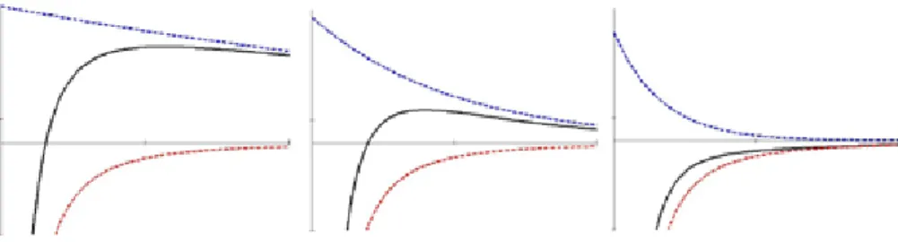
In the 1940s, Derjaguin, Landau, Verwey and Overbeek described the stability of lyophobic1 colloids in suspension in terms of electric double-layer and dispersion forces. This is summarized in the DLVO-theory where the total interaction energy between two colloids is the sum of the dispersion interaction energy and the electric double layer interaction energy. If two similar lyophobic surfaces are brought together in an electrolyte solution the electric double layers will act repulsively due to the increased ion concentration in between the surfaces as they approach each other, whereas the dispersion forces will act attractively. This can be demonstrated with interaction curves as shown in Figure 2.
1 The term lyophobic means that the dispersed particle does not interact with (“like”) the surrounding medium in which it is dispersed.
Figure 2. DLVO interaction between two similar surfaces approaching in electrolyte solutions of increasing ionic strength (left → right ). The upper (blue, dashed) curve is the EDL-interaction (repulsive), the lower (red, dashed) curve is the dispersion interaction (attractive), the middle (solid, black) curve is the total interaction. The abscissa represents the distance between the two surfaces.
In Figure 2, the repulsive double layer interaction decreases with increasing ionic strength (left → right), due to the shielding effect of the ions on the surface charge. The attractive dispersion interaction remains constant and the total interaction is therefore attractive at all distances at high enough ionic strength (Figure 2, right). At close contact the Born-repulsion will cause a large repulsion of the surfaces, not shown in the figure (see discussion above).
Steric effects and deviation from DLVO-theory
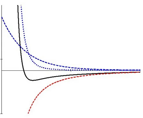
Refinements of the DLVO-theory take into account solvation and steric effects, which can manifest themselves as deviations from DLVO-behavior, e.g. oscillations in the force as the surfaces approach or repulsions/attractions not expected from pure double-layer or dispersion interactions. One such example is the influence of polymers present on the surfaces. If the polymers are readily soluble in the media in between the surfaces there will be a repulsive force, due to decreased entropy and increased osmotic pressure2, which follows when the polymers are compressed as the surfaces approach (Figure 3). Increased attraction between the polymer surfaces can also occur if the solubility of the polymer 2 Osmotic pressure is the pressure which makes water flow from diluted regions to
is low or the surface coverage of the polymer is poor. This can be due to entangling of the polymers, if they have a greater affinity to each other than for the solvent or due to adsorption of polymer molecules on both surfaces if the surface coverage is poor.
Figure 3. Steric repulsion of two surfaces coated with polymers readily soluble in the media in between the surfaces. The dashed blue curve is the EDL-interaction (repulsive), the dotted blue curve is the steric EDL-interaction due to the presence of polymers at the surfaces (repulsive), the dashed red curve is the dispersion interaction (attractive), the solid black curve is the total interaction (attractive → repulsive). The abscissa represents the distance between the two surfaces.
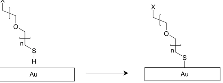
In the protein transport experiments, described in paper I, the surface of the chip as well as the beads have been coated with polyethylene oxide (PEO) to reduce interaction between the beads and the chip as well as to avoid
The good solubility of PEO in water promotes steric repulsion of the chip and bead surfaces due to non-DLVO repulsion.
Brownian motion
As the size of an object goes from centimeter or millimeter size down to the size of molecules, it will also change its physical behavior. The effect of random walk of a grain of sand is almost non-existent, whereas that of a hydrogen molecule is very large. It is somewhere in between these limits that micro- and nanotechnology has its domain. The randomizing effect of Brownian motion counteracts the electric-, magnetic- and surface-forces discussed above. The work described in this thesis is mostly concerned with micrometer-sized beads, so in the following section the random movement of a representative bead is described.
Brownian motion is the random motion of small particles that follows as a result of their collisionwith surrounding molecules. The mean displacement x of a particle due to Brownian motion is described by the equation
t D
x= 2⋅ ⋅
where t is the available time and D is the diffusion constant, which is dependent on temperature as well as the particle shape. For a spherical particle, the diffusion constant is calculated by the equation
a
T
k
D
⋅
⋅
⋅
⋅
=
µ
π
6
where k is the Boltzmann constant, T is the absolute temperature, µ is the dynamic viscosity and a is the particle radius.
The mean displacement in 1 s due to Brownian motion for a particle with radius 5 µm in water at 298 K is about 0.3 µm (or 6% of the particle diameter). As the particle size is reduced, the displacement increases. For a 1 µm particle the above calculation gives a mean displacement of 0.7 µm (or 70% of the particle diameter).The dynamic viscosity for water at 298 K is about 10–3 Ns/m2. The Boltzmann constant is of the order 1.38∙10–23 J/K. In paper I, III and IV particles between 1 and 5 µm are used. Some effects of Brownian motion can therefore be expected in those experiments.
3. Dielectrophoretic and magnetic forces
Dielectrophoresis
Dielectrophoresis is the phenomenon of motion of polarizable particles in non-uniform electric fields discovered by Herbert Pohl in 1951 (Pohl, 1951). Dielectrophoresis differs from electrophoresis in some fundamental aspects. Electrophoretic motion is induced by the Coulomb force acting on any charged object in a homogenous or non-homogenous electric field, whereas dielectrophoretic motion is induced by the force between dipoles in the object and a non-homogenous electric field. The most important differences are that for electrophoresis to work, the object needs to be charged, whereas for dielectrophoresis, the object must be polarizable (it can be either charged or uncharged). Finally, electrophoresis is performed in DC fields, whereas dielectrophoresis can be performed in both AC and DC fields.
Dipoles
Dipoles can be of two types: permanent or induced. In a permanent dipole, the dipole exists both in the presence and the absence of an electric field and is dependent on the atomic configuration of the molecule. Water and carbon monoxide are examples of molecules possessing permanent dipoles. Dipoles can also be induced in molecules: the electron cloud surrounding a molecule can be displaced relative to the nuclei (electronic polarization), or a charge can move between different positions in the molecule (atomic polarization), thus creating a dipole. In an induced dipole, the dipole can exist only in the presence of an electric field. By convention, dipoles are sketched from negative to positive ends.
Polarization
Polarization is a process in which a dipole aligns in an electrical field. In the case of a induced dipole, the polarization occurs as the dipole is induced (see above). A molecule possessing a permanent dipole can also align in the field by rotation of the molecule (orientational polarization). These polarization mechanisms are referred to as Debye polarizations. At higher frequencies of the alternating field, orientational polarization is not induced. For example, in the case of water, frequencies greater than a few GHz can not induce orientational polarization due to inertia of the water molecules.
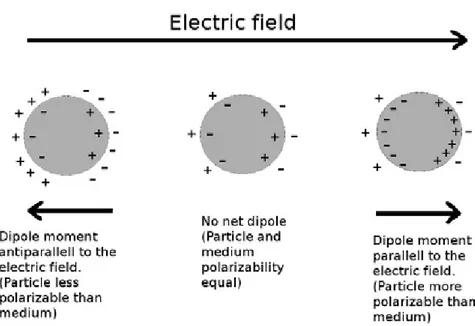
Consequently, the water molecule cannot reorient itself synchronously with the field. This causes a so called dispersion, which means that the orientational contribution to the total polarization is lost and only those polarization mechanisms with shorter relaxation times (atomic and electronic) contribute. Thus, as a polarization mechanism is lost in a material, the permittivity (dielectric constant) of the material is lowered. In dielectrophoretic applications the frequencies are in the lower range, kHz to MHz, and the above-mentioned polarization mechanisms (Debye, electronic and atomic) can be considered constant. Instead another polarization mechanism, the Maxwell-Wagner interfacial polarization, dominates. This type of polarization occurs when two materials with different polarizability share an interface (such as a particle suspended in a medium) are exposed to an alternating electric field. As a result of the two materials polarizing or conducting charge differently, there will be a charge build-up, polarization, in the interface between the two materials. In Figure 4, this process is shown for three cases: a particle with less, equal and higher polarizability than the surrounding medium placed in an electric field. In the case of an particle which polarize more easily than the surrounding medium, more charges are built-up on the inside than on the outside of the particle-surrounding interface (Figure 4, right). In the case of an particle which polarize less easily than the surrounding medium, more charges are built-up on the outside than on the inside of the particle-surrounding interface (Figure 4, left). The net induced dipole thus changes direction depending on the relative polarizabilities of the particle and the surrounding medium. If the electric field is reversed, the charges will move to the opposite sides, thus the induced dipole also reverse. At high enough frequencies the movement of free charges are too slow to keep pace with the change in electric field direction, and a relaxation thus occur. The remaining polarization mechanisms are then those with higher relaxation frequencies. These responses of the particles to the electric field are the basis of dielectrophoresis, as will be discussed in the following section.
The dielectrophoretic force
When a dipole is induced in a particle due to an external electric field according to the polarization mechanisms discussed above, there are two possibilities of what may happen to the particle from a dielectrophoretic point of view:
1. If the particle is placed in a homogenous field the net force on the dipole will be equal at both poles, and the particle will stay in place, i.e. nothing happens.
2. If the particle is placed in a non-homogenous field the force on the dipole will be unequal at the poles, and the particle will move. The direction of the movement will be determined by the direction of the induced dipole.
Figure 4: A polarizable particle placed in an electric field can
respond to the field in three different ways depending on the
polarizability of the particle relative to that of the medium: No
response (middle), dipole parallel to the field (right) or dipole
antiparallel to the field (left).
If the dipole is aligned with the field (Figure 4, right), the dipole is attracted towards higher field-strengths. If the dipole is opposing the field (Figure 4, left), the dipole is attracted towards lower field-strengths.
The dielectrophoretic force-vector, FDEP, on a dipole is given by
FDEP=(p·∇)E
where p is the induced dipole moment, E is the electric field and ∇ is the del operator3. If the field is changing in space (i.e. the gradient is non-zero), there will be a net force on the dipole.
If applied to a particle, the dielectrophoretic force vector will depend on 1. the electric field properties such as, strength, curvature and
frequency,
2. the particle properties such as size, shape and dielectric properties, 3. the dielectric properties of the surrounding medium.
The general expression for the dielectrophoretic force on a solid spherical particle suspended in a medium is (Morgan and Green, 2003; Hughes, 2003)
F=2⋅π⋅εm⋅r3⋅Re[K(ω)]⋅∇|E|2
where εm is the relative permittivity (dielectric constant) of the surrounding medium, r is the radius of the particle, E is the electric field (V/m) and Re[K(ω)] refers to the real part of the complex Clausius-Mossotti factor (Morgan and Green, 2003; Hughes, 2003),
K(ω)=(ε∗
p-ε∗m)/( ε∗p+2ε∗m) where ε∗
p and ε∗m refer to the complex permittivity of the particle and medium respectively. The complex permittivity is the permittivity corrected for the frequency dependence present in so-called lossy dielectrics. This 3 The del-operator, ∇, is the multi-dimensional analogy to the derivative. In three dimensions ∇ is defined as (∂/∂x, ∂/∂y, ∂/∂z). When applied to a vector field, the del-operator gives the direction and magnitude of the greatest slope of the field
means that the dielectric contains both a capacitive and a resistive component. In electrical terms this is in principle a capacitor and a resistor in parallel. At low frequencies the impedance is determined by the resistive component, whereas at high frequencies the impedance is determined by the capacitive component (see discussion of polarization above). The real part of the Clausius-Mossotti factor can take numbers between -0.5 and 1, which means that this factor is if importance in determining the direction of the dielectrophoretic force (Figure 5).
1 .104 1 .105 1 .106 1 .107 1 .108 0.5 0.25 0 0.25 0.5 0.75 1 Frequency C M -f ac to r
Figure 5. The real part of the Clausius-Mossotti (CM) factor at different applied frequencies. The sign of the CM factor changes from positive to negative slightly above 106 Hz, which means that the particle shows negative
dielectrophoresis above this frequency.
If the real part of the CM-factor is positive, the force-direction is towards high field strengths, whereas if it is negative it is directed towards low field strengths. In Figure 4, this is represented by the change in dipole direction from parallel to anti-parallel at increased frequencies (the particle behaves as an capacitor at high frequencies since the free charge-movement is too slow to keep pace with the field). This frequency dependence is of great importance, since it makes it possible to separate objects with different dielectric properties by choosing a frequency where Re[K(ω)] have different
signs for the two objects (Gascoyne and Vykoukal, 2002; Morgan and Green, 2003; Hughes, 2003).
Positive dielectrophoretic trapping
Once trapped by positive dielectrophoresis, a particle is moved towards higher field strength, and thus the trapping becomes stronger with time (until it is stopped e.g. by reaching the electrode edge) as the force on the particle is increased with the field strength (Hughes, 2003).
Magnetism
Magnetic field
Magnetic fields are generated by moving electric charges. One example is the magnetic field around a current carrying wire (Figure 6), where the magnetic field is produced by a net flow of electrons in the wire. Another example is the magnetic field around a bar magnet (Figure 7). Here, the origin of the magnetic field is the orbital and spin moment of the electron.
Figure 6. Magnetic field produced by an electric current in a wire.
Figure 7. Magnetic field produced by a bar magnet.
Magnetic field intensity, magnetic flux density, magnetization and magnetic susceptibility.
The magnetic field generated by the current in a wire as in Figure 6 is called the magnetic field intensity or simply the magnetic field, H (A/m). When the magnetic field is applied to a particular medium, the responding field is called the magnetic flux density, B (Vs/m2 ; Tesla, T).
The relation between B and H is expressed as B = µ0(H+M),
where µ0 = 4πּ10-7 (N/A2) is the permeability of free space and M (A/m) is the magnetization of the material defined as
M = ΧּH
X (-) is called the magnetic susceptibility of the material. Combining the two above equations yields
B = (X+1)ּH or
B = µrµ0H,
where the relative permeability, µr, (-), is related to X by µr = (X+1).
For a non magnetic material, e.g. in air, X = 0 (or µr = 1) and B is proportional to H.
The origin of magnetization in a material is of quantum mechanic origin and a full description of the phenomenon is outside the scope of this thesis, but a simplified model is given below.
Magnetic dipoles and magnetization
The electric dipole is, as described earlier, defined as two electric charges, electric monopoles, separated by a distance. The strength of the electric
dipole can then be defined as the product between the separated charge and the distance and has the unit [C*m].
Since magnetic monopoles are not defined, the description of a magnetic dipole is somewhat different from that of an electric dipole:
A magnetic dipole can be defined by a circular loop carrying an electric current, thus producing a magnetic field normal to the loop plane. The strength of the magnetic dipole can then be defined as the electric current through the loop times the area inside the loop and has the unit [A*m2]. In the classical atomic model, the electron orbiting the nucleus contributes to the total magnetic moment of the atom (or ion) in two separate ways:
• The orbital magnetic moment which is the effect of the electron orbiting the nucleus.
• The electron spin magnetic moment which is the effect of the electron spinning around its own axis.
For the transition elements, e.g. iron, the electron spin magnetic moment gives the major contribution to the total magnetic moment. In magnetic elements, the moments of the electrons add up to a total non-zero moment for the atom (or the ion). Hence, each atom (or ion) acts as a magnetic moment, or dipole. The magnetization is the total magnetic moment per volume in a material, thus it is given in [A/m].
Ferro-/ferrimagnetic materials and magnetic domains.
The dipolar interaction tends to order magnetic moments anti-parallel (cf. the behavior of two macroscopic bar magnets). However, in a ferromagnetic material, the neighboring atomic moments are ordered in parallel, due to a quantum mechanical based, short range interaction, called the exchange interaction.
This long-range/short-range interaction duality causes an energy trade-of which manifests itself in the following way:
In the ferromagnetic material there are areas, called magnetic domains, in which the magnetic moments are ordered in parallel due to the short range interaction. This causes a net magnetization of the material within the domain. However, due to the long-range dipolar interaction, striving towards the anti-parallel configuration, neighboring domains are ordered in other directions, which causes a zero total moment of the material (in the demagnetized state).
When the material is exposed to an external magnetic field, the domains with magnetization directions close to the applied field will increase in size (a large enough field can also change the magnetization direction within the domain). When the field is removed, the enlarged domains will not completely return to their original size. This is called magnetic remanence, and causes the material to keep a total bulk magnetization, even in the absence of the field.
The ferrimagnetic materials differ from ferromagnetic materials by the short-range ordering of magnetic moments, which are divided in both parallel and anti-parallel configuration in the ferrimagnetic material. There is, however, an imbalance in this ordering in the ferrimagnetic materials which causes a magnetic moment.
The introduction of magnetic domains in a material will also introduce areas, domain walls, within the material where the magnetization direction changes. The introduction of a domain wall costs energy since a material is more easily magnetized along certain directions, easy axes, determined by its crystal structure. If the atomic moments are forced to be directed in non-easy directions , as in a domain wall, the so-called magnetocrystalline anisotropy energy increases with the number of atomic magnetic moments. This will tend to make the wall thin. If the change in moment direction between adjacent atoms is small, there is less cost in exchange energy between adjacent atoms. This will tend to make the domain wall thick, since more atoms are needed in the domain wall to make the change in direction between each atom small. Therefore, the domain wall thickness will be a bargain between minimized anisotropy energy and minimized exchange energy. If a magnetic crystal is small enough, it cannot contain a domain wall since the wall must be of a finite thickness. The result of this is a single domain crystal, i.e. all magnetic moments point in the same direction. The size of a single domain is material-dependent, but about 50 nm is common. Superparamagnetism
When the size of a single domain is reduced, there will be a point where it cannot keep the magnetization direction when the magnetizing field is removed and the magnetization will constantly change direction and behave very much like a large paramagnetic atom4. When the single domain particle 4 Paramagnetic atoms have unpaired electrons, which cause a net magnetic
shows this behavior it is said to be superparamagnetic. The size of a superparamagnetic particle is material-dependent, but sizes below about 15 nm are common. Superparamagnetic particles are important in magnetic bead technology, because of their lack of magnetic remanence.
4. Methods
Electric conductivity measurement
When an electric potential (U) is applied over a piece of conducting material, there will be a drift of charges in the field due to the electric potential. This drift of charges, the electric current (I), is related to the potential by Ohms law
U K
I = ⋅
where the conductance, K, describes how much charge a specific piece of material transports at a given potential. Its reciprocal is the parameter resistance (R), which give Ohms law the familiar form
R I
U = ⋅
The resistance can be expressed as
A
l
R
=
ρ
⋅
where l is the length of the sample, A is the cross-section and ρ is the resistivity, which is a material-specific parameter. In terms of conductance the expression takes the form
l
A
K
=
κ
⋅
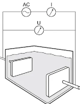
where κ=1/ρ is the conductivity. Electric charge can be transported as free electrons, as in metals, or as mobile ions, as is in an electrolyte solution. A conductivity meter for measurements on electrolyte solutions consists in its simplest case of a measurement cell, an electric power source and some type of resistance analyser (Figure 8).
Figure 8. Principle of a conductivity meter. The resistance (or conductance) of the solution is measured with a voltage and current meter (by Ohms law). With knowledge of the cell constant, given by the geometry of the cell, the conductivity can be calculated. Figure courtesy of Endress+Hauser, Germany.
The geometric term, A/l, is called the cell constant, and depends on the sensor geometry. If the cell constant is known, the conductivity can be determined by a simple current-voltage measurement. The cell constant can be determined experimentally by measurements on conductivity standards. In paper II, a conductivity meter (Conducta CLS-TSP 3567, Endress+Hauser, Germany) has been used to measure the conductivity of bacterial suspensions.
To avoid redox reactions at the electrodes of the conductivity meter, an alternating current with a frequency in the kHz range is used for the measurements. The value obtained will be the impedance with frequency-dependent contributions from capacitive and conductive elements in the solution. The measuring frequency is set by the software in the instrument. Since the conductivity is temperature-dependent, about 2 %/°C, the temperature must be under strict control. During the measurements, the temperature is controlled by both a built-in temperature probe in the conductivity sensor and by an external PT-100 sensor. Prior to the