Sweden’s Commodity Export Potential - A Gravity Approach : South-Korea

J

I

B

S

JÖNKÖPING UNIVERSITY

Sweden’s Commodity Export

Potential- A Gravity Approach

South-Korea

Bachelor thesis within economics Author: Per Drottz

David Lantz

Bachelor’s Thesis in Economics

Title: Sweden’s Commodity Export Potential - A Gravity Approach South-Korea

Author: David Lantz Per Drottz

Tutor: Charlie Karlsson Professor Lina Bjerke Ph. D. Candidate Date: January 2008

South Korea, Trade potential, Gravity model, Sweden, Export

Abstract

This bachelor thesis aims to estimate Sweden’s export potential towards South-Korea since initial data indicates that Sweden has from 1997 up until 2005 been exporting less to South-Korea when compared to, in general, OECD. Furthermore, South-South-Korea seems to be a low prioritized market for Swedish firms in the East-Asian region. As many before us, we have used a basic gravity model, including GDP and distance in kilometer has been used as explanatory variables for the observed trade value. The dummy variable land-locked, to es-timate trade potential for 15 commodity groups. Sweden was set to be the exporting coun-try, South-Korea the importing country together with all the other OECD members, which were used as points of reference.

The outcome of the gravity regression shows that distance and the dummy variable land-locked (if a country does not have access to open water) have a very strong relationship to the observed export data. However, GDP was proven to have a very weak relationship to the observed export data thus making the estimation process of trade potential for all, ex-cept one, commodity group biased.

The gravity model has been widely criticized for inflating export potential due to misspeci-fication a problem that we experienced when running our regression. Thus, from this study no strong conclusions can be drawn concerning the trade potential from Sweden to South-Korea.

J

I

B

S

JÖNKÖPING UNIVERSITY

S v e r i g e s Va r u e x p o r t p o t e n t i a l

-E n G r a v i ta t i o n s u p ps k a t t n i n g

Sydkorea

Kandidatuppsats inom Nationalekonomi

Författare:

Per Drottz

David Lantz

Handledare: Charlie Karlsson, Professor

Lina Bjerke, Ph. D. Candidate

Kandidatuppsatts inom Nationalekonomi

Titel:

Sveriges Varuexportpotential- En Gravitationsuppskattning

Sydkorea

Författare:

David Lantz

Per Drottz

Handledare: Charlie Karlsson Professor

Lina Bjerke Ph. D. Candidate

Datum:

januari 2008

Ämnesord: Sydkorea, Handelspotential, Gravitationsmodell, Sverige, Export

Sammanfattning

Den här kandidatuppsatsens syfte är att uppskatta Sveriges export potential till Sydkorea då

initial data indikerar att Sverige har, generellt sett, under de senaste åren tappat mark

gentemot OECD. Sydkorea verkar vara en lågt prioriterad marknad i Östasien bland

svenska företag. Så som många före oss har vi använt oss av en simpel gravitationsmodell,

den inrymmer BNP och distans mätt i kilometer som beskrivandevariabler samt

dummyvariabeln land-låst, för att estimera handels potentialen för 15 varugrupper. Sverige

sattes som exporterande land, Sydkorea som importerande land tillsammans med all de

andra OECD medlemmarna som användes för referens punkter.

Resultatet av gravitationsregressionen visar att distans och dummyvariabeln land-låst har en

väldigt stark relation till observerad exportdata. Däremot visades att BNP har en väldigt

svag relation till observerad exportdata vilket gjorde uppskattnings processen av handels

potentialen för alla varugrupper med undantag för en irrelevant.

Gravitationsmodellen har blivit vida kritiserade för att blåsa upp exportpotentialen på

grund av misspecificering. I våran strävan att undvika så mycket misspecificering som

möjligt bestämde vi oss för att använda oss av de mest använda variablerna, så som tidigare

nämnt. Detta löste inte problemet då det istället förvärrade problemet och vi i slutändan

blåste upp vår estimerade handels potential värden.

Slutligen lider våra resultat av för många irregulariteter vilket gör det omöjligt för oss att

dra straka slutsatser gällande handels potentialen mellan Sverige och Sydkorea.

Table of Contents

Bachelor’s Thesis in Economics ... i

Abstract ... i

Table of Contents... ii

1 Introduction ... 1

2 Theoretical Framework ... 4

2.1 Trade Liberalization ...4

2.2 Why Distance matter ...5

2.3 Network economics ...6

2.4 Summary of theories and hypothesis ...7

3 Empirical Framework... 9

3.1 The Gravity model ...9

3.2 Data Source ...12

3.3 Regression Model – Panel data ...14

4 Analysis ... 16

5 Conclusion ... 19

6 Further research... 20

References ... 21

1

Introduction

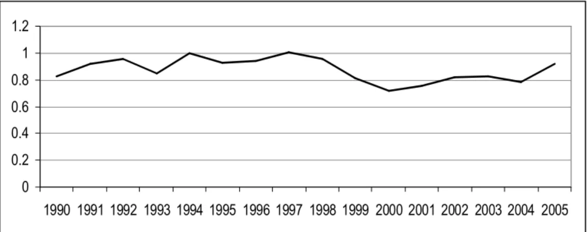
Since 1996, Sweden has experienced a sharp negative trend in their trade balances with Ko-rea*_{, in terms of trade value. However, we also find that the trade balance has stabilized in} recent years ending up at a point where Sweden’s export to Korea is almost equal to Ko-reas export to Sweden (Appendix 1).

Until June 1997 all East-Asian currencies, with the exception of the Japanese yen, were pegged to the US dollar and when they became floating, according to McKinnon (2001, p 2), that led to a “…sharp currency devaluations of Indonesia, Korea, Malaysia, Philippines, and Thailand—and the collapse in their demand for imports…”. Furthermore, Krugman (1998, p 1) explains that the currency crises are not the only explanation of the decrease in East-Asian economies. He argues “What we have actually seen is something both more complex and more drastic: collapses in domestic asset markets, widespread bank failures, bankruptcies on the part of many firms, and what looks likely to be a much more severe real downturn than even the most negative-minded anticipated.”

The East-Asian crises had an enormous effect on Korea. This in turn led to a downfall in demand especially during the years of 1997 and 1998. One conclusion that can be drawn from this period is that the demand for imports declined explaining the development in the trade balance between Korea and Sweden.

In 1999 the major parts of the financial crises was over for Korea. GDP growth in Korea was more than 10 percent due to healthy exports. There was a great increase in Korea’s imports from some regions and they were the two Asian nations, Japan and China, and North America. The slower regions was Europe but also Oceania. The growth of the ex-ports was mostly goods as semiconductors and automobiles. The imex-ports consisted of cap-ital goods thanks to the great optimism in Korean market. There was a high confidence in the Korean market from the recovery from the Financial Crises and the recession that had followed (Junsok & Hong-Youl 2000).

There was a great deprecation in the value of the Korean Won in the year of 1997 before it stabilized in 1999. This depreciation in combination with decreased wages due to recession and structural adjustments that had followed the Financial Crises increased the competi-tiveness of Korean exports considerably. This competicompeti-tiveness also gave the market a lot of trade friction. Imports were the biggest problem within in the trade account. In the year of 1998, imports fell and Korean firms faced a recession. Korea faced higher import prices af-ter the recession. There were two major reasons why Koreas import prices increased. First, Korea restructured its banking sector. Secondly, the fall within the import sector was also appeared greater due to the world deflation in prices of raw materials and looked bigger in order to be seen under unit value then volume. In 1999, there was a significant rise in the number of Korean firms. There was both an increase in imports of capital goods and con-sumption goods (Junsok & Hong-Youl, 2000).

In 2000 some of the structure problems remained within Korea’s imports and exports due to the financial crises. The financial sector was still struggling due to high debts to

bols†_{. There was also a downturn in investors because of a lack of confidence, especially} within the financial sector (Junsok & Hong-Youl, 2000).

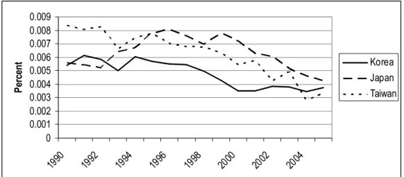
When comparing Sweden’s export to Korea with OECD’s export to Korea, then excluding Czech Republic, Hungary, Poland and Slovak Republic, in Figure A2 (see Appendix) we find that for the period, 1990-2005, that Sweden’s export to Korea has declined more than OECD’s export to Korea. Furthermore, when comparing Sweden’s export to Korea with other similar markets in the region, Japan and Taiwan suggested by Whitley (1992), throughout the same period in time in Figure A2 (see Appendix) we find that the export to Korea has been significantly lower than to Japan and Taiwan. However, the distribution of Swedish export in the region has gone towards equalization in respect to the recipient countries GDP in recent years.

In later years, empirical studies of international trade relationships have become more pop-ular such as the ones conducted by Christie (2002), De Benedicts and Vicarelli (2005), and Sohn (2005) where the gravity model have proven to be a good tool for estimating trade positional in the case of bilateral trade.

In his article, Christie (2002), when estimating the trade potential in South-East Europe, concludes that the gravity model has provided to be a clear benchmark for potential trade level analysis based on economical size and geographical distance. De Benedictis and Vica-relli (2005) use an example of trade flows where they have been using 11 European coun-tries and 31 OECD ‘reporting’ councoun-tries. They conclude that trade potentials might de-crease or give a rise to successful trade relations. Sohn (2005) examines if the gravity model can explain changes in Koreas trade flows in recent years. He uses a sample of 30 major trading partners and reached the conclusion that Koreas economy has been growing rapidly mainly from expanding its trade flows. They have been expanding from a small economy with few resources to a world economy.

Rivera-Batiz and Olivia (2003) examines previous studies were the gravity model has been used and stresses that countries that trade within a regional trade agreement tend to shift away from the rest of the world. This kind of trade agreements usually occur between countries which are natural trading partners and that are geographically close to each other. However, we have not found any empirical studies explaining the trade relationship be-tween Sweden and Korea. Regardless of what has happened to the state of the East Asian region’s economy over the last 15 years the data presented in Figures 2 and 3 indicate that Sweden has never reached its full export potential to Korea. However, we have observed, a closing of the gap has accrued in later years see Figure A1 (see Appendix).

The purpose of this thesis, is to estimate Sweden’s export potential towards the Korean import market and then compare those findings to actual trade data in order to identify whether or not Sweden has managed to fully penetrate the Korean import market. Fur-thermore, if the import market is not fully penetrated, how great is the difference between the potential level of penetration and the actual level of penetration.

The thesis is organized as following. In section two, theoretical Framework presents theo-ries of trade, trade liberalization, why distance matters, network economies and empirical finds are presented and discussed in order to determine what factors needs to be taken into account when determining patterns of trade and how they occur.

Section three introduces the gravity model and empirical findings where the gravity model has been applied in order to determine trade potential and the risks of misspecification is presented and discussed. Furthermore, our data selection presents a gravity model that is modified to fit the purpose of our thesis. In the last part of this section, we discuss the plications of our gravity model, regression model, and the econometrical challenges it im-plies.

Our results are presented and discussed in section four and our conclusion is drawn in sec-tion five.

2

Theoretical Framework

This section will present theories concerning international trade and the effects distance, geographic transactions cost, and the of international networks has on imports and exports between countries. This will be done in order to explain how the gravity model can be ap-plied to estimate trade potential using panel data.

2.1

Trade Liberalization

According to the economic concept of perfect competition, trade reform is beneficial and a liberal trade regime can boost a country’s economy. At the same time as trade liberalization start, there will be an increase in trade between countries which will open up both for im-ports and exim-ports. Some of the benefits from trade liberalization are that a country is able to improve resource allocation, access to better technologies, inputs and intermediate goods. There will be greater domestic competition and ability for externalities like transfers of knowledge. A small country will under perfect competition gain by eliminating tariffs. Resources is used more wisely because there will not be any production of goods that can be imported at a lower price. Free trade usually leads to a more cost-effectively balanced market structure. The gains from liberalization also come from scale economies. Protec-tionism can create market power for domestic firms where under free trade there would have been none. Trade liberalization opens up opportunities because of the ability to get cheap inputs in order to create export opportunities. Investments can be made in capital goods from the rents, profits from exports, and later serve productivity gains (Dornbusch, 1992).

Kim (1996) found when trying to identify visible costs of protection in the Korean market that it had been a, more or less, closed market up until the 1970ies. However, it was in the late 1970s that the Korean government started to encourage competition by slowly opening up the market to international competitors in order to advance the efficiency of the econ-omy. Korea’s trade is regulated under the Foreign Trade Act and the Customs Act. With this approach, Korea can only regulate imports consistent with international trade agree-ments. The achievement is to promote external trade and maintain fair trading practices consistent with international trading rules. The Foreign Trade Act regulates imports and exports. This works under the system of Export-Import Public Notices, which refers to the import liberalization ratio.

The author concluded that there would be a consumer surplus when imported and domes-tic goods decrease its prices due to tariffs removal of protection. The biggest consumer gains are within the agricultural and fishery products. The increased imports results from trade liberalization and lowering of tariffs. Labor and capital will move from protected areas to other parts of the economy. This improvement will increase the exports from the sectors with a competitive edge. Domestic production will decline specially within the agri-cultural and fishing sectors that have a high level of protection. Sectors within machinery, metal products and textile industries will also be hit hard. The reaction of lowered tariffs will hit the domestic employment. The agricultural and fishing sector will reach the largest fall within employment (Kim, 1996).

2.2

Why Distance matter

Rivera-Batiz and Olivia (2003) argues that the greater the distance between two trading partners the greater the transport cost. This makes sense because trade decreases when dis-tance between two countries increase with higher transport costs. The amount of trade is dependent on the countries income and size.

Ghemawat (2001) divides distance between countries and therefore divides exports and imports between countries in four groups; most common is geographic but also of cultural, political and economic dimensions. All these parameters within trade are able to make a foreign market less attractive. Both traditional economic factors including wealth and size (GDP). Other factors are much more relevant in order to increase trade. Countries that are closely related culturally and administratively have higher amount of trade. Countries that have a common membership in a regional trading bloc increases trade more than countries with different currencies. Geographic distance affects the communication and transporta-tion. The cultural attributes decide how people interact. The distance in people’s religious beliefs, social norms and language creates distance between two countries. This will show how likely it is for countries to open up for trade between each other. Cultural differences affect consumers’ product preferences. Political and administrative barriers depend much on a history point of view. Policies of individual governments pose the most common bar-riers to cross-border competition. A government that raises barbar-riers to foreign competition such as tariffs, restrictions on foreign direct investment and trade quotes is able to protect domestic industries. The geographical distance depends a lot on the countries size, distance to borders and access to ocean and topography. The further away from a country the hard-er it is to trade between countries.

Johansson, Karlsson and Stough (2001), write that products usually exchanged under com-plex transaction costs. Distance includes both transportation and the transaction cost, which consist of geographic distance between seller and customer. Transaction cost might be very complex to deal with and are in many cases not standardized, examples of this are inspection, negotiation and legal consolation. Transaction cost might decrease after re-peated interaction between provider and customer. Development of new product variants and production in order for sails of the established products is the main activity of a firm. This is usually due to relations with other firms and other sectors. Many relations occur within suppliers and their customers.

The demand for variety increases as income grows. The larger differentiates in the income per capita within a region, the larger are the differentness in opportunities in that region. In a case where there are more economic links between actors, it is likely for new links to be established. Externalities that influence the size of affinity coefficients are cultural, lan-guage, communication distance, distance as regard to income level, life style and consump-tion pattern. Interacconsump-tion costs associated with nearby contacts and the existence of estab-lished economic networks between firms in each pair of regions. Trade affinities are a gen-eral phenomenon that influences economic links and trade links influenced by already es-tablished patterns (Johansson, Karlsson and Stough, 2001).

Today, economies interact more and more with one and other and thus they cannot be re-garded as isolated islands. In order to generate innovation it is very important to realize its linkages from regions to other parts of the world. Embedded in competitive advantage is learning of habits, rules and norms such as social capital and entrepreneurial traditions. There will always be a need to create new knowledge in order to create trust and

confi-dence for regions to build new relationships. Factors that are responsive to innovation in-clude factors from infrastructure that supports activity patterns and governments that have a solid financial community in order to start business. Some of the parts of soft infrastruc-ture or intangible infrastrucinfrastruc-ture are social capital that usually includes awareness and insti-tutions. The institutions illustrate individual’s action, collective beliefs and moral rules. These steps influence the transaction cost and will be able to reduce cost such as negotia-tions, contract information and search adjustment (Johansson, Karlsson and Stough, 2001). In order for firms to grow, gain profits and survive, they need to import goods that are cheaper to produce in the foreign country and export goods that are cheaper to produce domestically. The advantages for firms generate gradually over time and regional advantag-es can be used for labor with special skill and high education. The affinitiadvantag-es and barriers outline and influence the establishment of customer links in order to form aggregate pat-terns of flows (Johansson, Karlsson and Stough, 2001).

2.3

Network economics

Although distance matter scholars, Johansson and Mattson, 1988, Meyer and Skak, 2002 among others, argue that the impact is has on international trade has decreased over time. Under the concept of networks and networking, which has become more and more popu-lar within the field of economics and other sciences in recent years, driven on by the im-portant role that networks play in todys society. (Johanson, Karlsson and Westin, 1994) Networks are not coordinated by market activities nor by a hieratical system. They are ra-ther based on trust and mutual interests between actors who interact with one anora-ther in a network setting (Johansson and Mattson, 1988). Business networks, and firms that take part in business networks, are very much liked to and are dependent on the society they are located in, the so-called national society and the culture it is based on. Cultures respond to interactions with other cultures and thus this will also affect the national business network, hence the internationalization process of the business network coevolves with the interna-tionalization process of a firm. (Meyer and Skak, 2002)

This reasoning shows the importance of networks and how it relates to international trade. Johansson, Karlsson and Westin, (1994, pp. 2) also emphasize on the importance of net-works in today’s society and in the field of economics the following three processes are of highest importance:

 The increased intensity and complexity of human interaction.

 The decreasing importance of geographical territory as a determinant of accessibili-ty.

 The failure of markets as a means to solve inter-firm relations when customized commodities are developed in complex environments

The rapid evolution of communications, and thus the information system, travel and trans-portation has made the world smaller. Trade partners located, in what was considered to be, remote parts of the world to distance to conduct trade with are now not more than a phone call or an email away. This have give rise to new opportunities and relationships across borders has begun to form. More and more efficient ways of logistics has started to replace the old ways of production and the strive for economies of scale. The economy as a whole is undergoing mayor structural changes and in order to be prepared to what might

come it is important to understand the driving force behind it all and thus the importance of network economies. (Johansson, Karlsson and Westin, 1994)

Johansson, Karlsson and Westin (1994) made a thorough revive of network literature re-lated to the field of economics and the empirical finds in them. According the authors, the analysis of infrastructure networks different production systems and special input-output models are observed within network economies. This deals with interaction among the so-ciety, economic networks and communication systems. There need to be analyses of why and when network economies are shaped and how they will be maintained in order to coo-perate and compete. It is also important to see the synergies between networks and other interactive structures. The concept of network economies also involves the process related to social economics. The process includes the understanding of the way information and communication technologies, our increased mobility and the demand for variety as income grows. The network economies deal with the patterns in a new and differentiated society. This also includes how we need to increase the understanding within this field. The interna-tional trade needs to include and analyze new barriers, accessibility and the complexity that is the reason for interaction that is not always directly connected with geographical dis-tance.

The author also emphasizes that a country will gain a comparative advantage for both the export producing and the technology delivering sectors due to a close interaction between suppliers and customers in a country. Here the knowledge can be both transferred through university but especially through learning by doing. They also emphasize the importance that the exporting countries supplier and customer links is very important in the relation for the increased global integration. We also need to include the effects of friction, barriers and affinities, because international trade is not as homogenous as in trade theory. Differ-ent forms of friction, affinities and barriers will reflect the sensitivity on a firm’s market performance. Johansson and Westin also argue that cultural trade affinities until effect that has differentiated commodity in a sector that has growing employment. Distance and common borders affect goods that price competitive. A product that is in innovation stage of the product cycle is more dependent on the affinities. The early stage is therefore an im-portant step in the establishment of network economies. (Johansson, Karlsson and Westin, 1994)

2.4

Summary of theories and hypothesis

To summarize the theoretical section we can conclude that when looking for patterns in in-ternational trade we need to take into account, who produces what and why. To illustrate further, which are the country specific resources and how it lead to country specification in terms of production. In relation to international trade, we also need to take purchasing power parity in to account. In reality, since there is no such thing as perfect competition in the world, we need to consider trade policies. Are there any trade agreements between Sweden and Korea, and are there any tariffs or any other trade barriers? We can break it down even further, as discussed by Ghemawat (2001) and Johansson, Karlsson and Stough (2001), what the actual transition cost of trade are between Sweden and Korea. What are the cultural differences such as language differences, religious differences, and political dif-ferences, international networks and how does that affect trade between Sweden and Ko-rea.

Hypostases’ 1: Through the evolution of international business networks physic distance and

transaction cost, such as cultural and political differences, will decrease over time.

Hypostases’ 2: Since physic distance will decrease over time, markets geographically far way

will historically be under penetrated.

3

Empirical Framework

The empirical test aims to identify the export potential from Sweden to Korea and how it has been affected by changes in Koreas GDP, transport cost, changes in Korean import ta-riffs, and other import barriers. This section also includes the selection of data and our re-gression model.

3.1

The Gravity model

The gravity model has become more popular over time and it has been widely used in in-ternational trade as an instrument for empirical studies. Today the gravity model is “... the workhorse for empirical studies ...”,(Eichengreen and Irwin, 1997 p33).

Tinbergen (1962) and Pöyhönen (1963) independently developed the gravity equation that applies to international trade and in 1966, Linneman developed the equation further by in-cluding population as a measurement of a country’s size. This simple form of the gravity equation can be defined as bilateral trade between two nations which is dependent on each other’s GDP, taking distance and sometimes other factors into account (McCallum, 1995). Krugman and Obstfeld (2006) define the gravity model as follows:

Tij= A * Yia * Yjb/ Dijc (3.1)

A is a constant term, Tij is the value of trade between country i and country j, Yiis country i’s GDP, Yjis country j’s GDP, and Dij is the distance between the two countries. The vo-lume of trade between two countries explains three different parameters. First, there is the size of the two countries’ GDPs and secondly there is the distance between the countries and lastly inversely proportional to the distance. The trade between two countries is pro-portional to the production of their GDPs and they diminish with distance (Krugman and Obstfeld, 2006).

Large economies usually spend large amounts on imports since they have high incomes. These economies also attract other countries to spend because they produce a wide range of products. A country’s share of world GDP is equal to the value of the goods and service it sells and therefore equal to what it produces (Krugman and Obstfeld, 2006).

The gravity model has become popular in the last decade due to its natural ability to project bilateral trade relations. The gravity model explains bilateral trade by GDP and GDP per capita figures and then takes distance and preference factors into account such as common border, language, etc. It was first applied to predict trade relations between OECD mem-bers and Central and East European countries after the iron curtain had fallen (see Wang and Winters, 1991; Hamilton and Winters, 1992; Baldwin, 1994; and others) (Egger, 2002). There have been two different concepts provided. In the first approach it was argued, by Wang and Winters (1991), Hamilton and Winters (1992) and Brulhart and Kelly (1999), that in the economic transformation of Central and East European countries (CEEC), these countries performed in another way than developed countries as the EU or OECD members. The gravity model estimates for EU or OECD countries in order to predict trade relations to CEEC’s. The difference between the observed value and the predicted value equals the trade potential between the countries. The other approach has been used more recently and there authors have included the transformation countries in regression

analysis. Then the residuals will be interpreted as the difference between potential and ac-tual bilateral trade relations (Baldwin, 1994; and Nilsson, 2002).

Christie (2002) uses the gravity model in order to estimate the trade potential in South-East Europe and concludes that the gravity model has provided a clear benchmark for potential trade level analysis based on economic size and geographic distance. In a small part of the paper Christie experiments with an alternative approach were instead of GDP, he uses GDP at PPP and instead of distance, he uses a matrix consisting of transport nodes. He ar-gues that GDP at PPP might better illustrate a trade relationship between certain countries since trade are sometimes conducted at different local prices. The argument for the use of a matrix of transport nods is that it is a better measurement of the actual transport cost when compared to the more classical approach of measuring distance between capital cities. He later concludes that his alternative gravity model did not outperform the classical set of va-riables.

Sohn (2005) uses the gravity model in order to extract implications regarding trade policies related to South Koreas bilateral flows. In his version of the gravity model, he uses both the Heckscher-Ohlin model and an increasing returns model. Therefore, the gravity analy-sis in this paper is critically dependent on Korea’s specific tradepatterns. The paper also in-cludes an Asian pacific trade network. The empirical analyses accomplished by 30 major trading countries of Korea in order to first provide a long run equilibrium view on trade flows.

Sohn, (2005) concludes that Koreas economy has been growing rapidly mainly from ex-panding its trade flows. They have been exex-panding from a small economy with few re-sources to a world economy. The empirical results show that the Hecksher-Ohlin model can explain trade flows. However, their trade flows are better explained by comparative ad-vantages, income difference and economies of scale within different development stages and product varieties. Koreas inter industry trade depend on standardized products. The Asian-Pacific trade flows show a significant positive effect on Korea’s trade volume. This means that there is a large intra-regional trade flow. There is an unrealized trade potential towards Japan and China.

Egger (2002) tries to provide insight to how to choose an adequate estimation technique for in-sample trade projections. According to him, in order to avoid misspecification “…the estimator choice is an important issue for the interpretation of the gravity coeffi-cients, which depends on the underlying interests.”(Egger 2002, p298) He considers three econometric problems for future research. The first part that easily can be mis-specified is the time-averaged cross-section in the gravity model because they ignore presence of ex-porter and imex-porter effects without its relevance. The second problem that is the compari-son of estimating results from different econometric concepts. This refers to the use of dif-ferent time horizons in the value of trade flows that change in the explanatory variables. Thirdly, Egger suggests that large systematic difference between observed and in sample forecast trade flows. This points to misspecification of the econometric model instead of unused trade potentials (Egger, 2002).

De Benedictis and Vicarelli (2005) apply, in their study, the gravity model when examining trade flows between 11 European countries and 31 OECD ‘reporting’ countries. They ac-knowledge Egger’s remarks on the risks of misspecification in their article “Trade Poten-tials in Gravity Panel Data Models” and that it often leads to inflated trade potential values and they state; “the very existence and the quantification of potential trade may be inflated

by problems of misspecification in the regression. Careful analysis of the specification is therefore needed if proper assessment is to be made of the presence and magnitude of bila-teral trade potentials.”(De Benedictis and Vicarelli 2005 p4.)

In order to avoid misspecification De Benedictis and Vicarelli consider “…an unobservable element which is country specific but not time invariant and which may affect bilateral trade flows together with covariates. It is generally hidden in the residuals and cannot be eliminated by fixed-effects.” (De Benedictis and Vicarelli, 2005 p3).

Furthermore, they also conclude that some degree of misspecification is unavoidable due to the problem of estimating the true market potential. (De Benedictis and Vicarelli, 2005) De Benedictis and Vicarelli formulated their model in the following way:







,'

'



'

z

,

y

where

y































h

u

u

h

u

z

x

x

y

the trade agreement dummy were 1 is the value if there is a trade agreement or 0 if there is not

z

measured in Km between the capital city of the exporter and the capital city of the impor-ter and a border dummy were 1 is the value if the exporimpor-ter and the imporimpor-ter share a border or 0 if they do not. εijt∼ i.i.d.(0, σ2ε).

x

y

u

, where

u

Where αiare unobserved over time invariant importer country level effects, αjare unob-served time variant exporter country level effects, αijare unobserved time invariant bilateral country-pair effects and the error term Eijtis independently, identically distributed over i and t and the, with the mean zero of variance, σ2

ε. All time invariant terms in equation

above were dropped and included in α.

ε

∼

i.i.d.(0, σ

ε

)

Export figures are presented in dollar terms at current prices. (De Benedictis and Vicarelli, 2005)

They estimated this equation using a simple OLS estimator and corrected it for White hete-roskedasticity. Furthermore, they used the estimated coefficient when calculating an in-sample trade potential index, x℘ _ijt:

ijt ijt x x jt

ê

e

x



A positive index value, a value greater than 1, shows a greater bilateral trade effect than predicted. A negative value, a value smaller than 1, shows a smaller bilateral trade effect than predicted. Finally, a value equal to 1 shows a bilateral trade effect that is equal to the predicted value (De Benedictis and Vicarelli, 2005).

They conclude by using this method that changes are substantially greater when country heterogeneity and dynamics are take into consideration. Trade potential might increase or decrease over time. Trade potential might decrease or give a rise to successful trade rela-tions. In order, for trade potential to emerge or rapidly exhausted it identifies when it ob-serves over a long time dimension. It is irresponsible to draw the implication of trade poli-cy if there is a lack of evidence of regularly untapped trade potential or the partnerships have not been observed over time (De Benedicts and Vicarelli, 2005).

To summarize this part of the empirical framework we can conclude that scholars in the field of international trade have frequently used the gravity model and it has been very suc-cessful when estimating trade potential. Furthermore, it has been widely criticized for in-flating trade potential due to misspecification, discussed by Egger (2002). To avoid misspe-cification completely is impossible, as noted by De Benedicts and Vicarelli, (2005). Howev-er, we can draw the conclusion that in order to avoid misspecification as much as possible we will try to make our gravity model as simple as possible. This however is contradicting to conclusions drawn in the previous section since it implies excluding many variables such as purchasing power, language differences etc. However, we feel that this is crucial for us to do in order to avoid inflating trade potential.

3.2

Data Source

The years selected for our study are 1997 to 2003, according to data availability. Further-more, the commodity groups were selected based on two digit SNI‡ _{codes; raw material} and other commodities that are traded on commodity exchanges were excluded. These goods were excluded due the fact that the origin or the destination of a good is of little im-portance and can then not be affected by the trade relationship between two countries. Furthermore, some limitations made due to data availability. In the end we selected; tobac-co, textile goods, clothes manufacture of fur, leather, publishing related goods, rubber and plastic goods, fabricated metal products, machinery, office supplies and computers, beve-rage, electrical components, manufacture of telecommunication, medical and optical in-struments, motor vehicles, other vehicles and furniture.

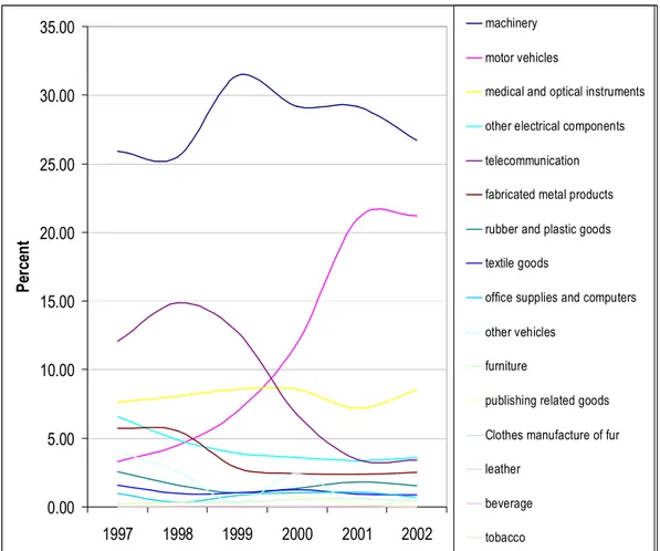
These commodity groups represent roughly 70 percent, varies slightly between the years, of the total export from Sweden to Korea. As can be seen in Figure A4 (see Appendix) most of the commodity groups have represented a, more or less, constant share of Sweden’s

port to Korea with a few exceptions, machinery, motor vehicles and manufacture of tele-communication. Machinery is by far the largest commodity group and represented 25 per-cent of Sweden’s total export to Korea in 1997, reached its peak in 2000, 31 perper-cent and then declined slightly to a level of 27 percent on 2003. Manufacture of telecommunication is the biggest loser apart from an initial increase from 12 percent in 1997 to 15 percent in 1999 it has continuously been losing ground and reached its all time low in 2003 then only representing 3 percent of Sweden’s export to Korea. Motor vehicles on the other hand is definitely the star of 1997, then only representing 3 percent of Sweden’s export to Korea and through a steady increase it reached 21 percent in 2003. The same patterns can be found when looking at export data in SEK, Table A1 (see Appendix).

In this study we have chosen to compare trade data from Sweden to Korea with trade data from all of the original OECD members to Korea. The reason for this is due to data avail-ability and since member ship in the OECD shows that a country has reach a comparable level of development to that of Sweden. To quote Eszter Hargittai, ”The OECD is an ideal case for investigating the ... represent advanced capitalist countries and thus membership controls for a general level of development. ...” (Hargittai, 1999 p5).

As mentioned previously in the introduction Sweden’s export to Korea with that of the OECD’s , then excluding Czech Republic, Hungary, Poland and Slovak Republic, in Figure A2 (see Appendix) we find that for the period, 1990-2005, that Sweden’s export to Korea has declined more than OECD’s export to Korea. Even though Sweden’s has not been as successful in Korea as the rest of the OECD the Swedish import penetration has risen from 10 percent in 1990 to a level of 17 percent in 2005, after controlling for country size, per capita income and transportation costs. Furthermore, when comparing Sweden’s ex-port to Korea with other similar markets in the region, Japan and Taiwan (Whitley 1992), throughout the same period in time in Figure A2 (see Appendix) we find that the export to Korea has been significantly lower than to Japan and Taiwan. However, the distribution of Swedish export in the region has gone towards equalization in recent years.

After the Asian financial crisis in 1997, Korea lowered its entry barriers and deregulated its market. This deregulation lowered tariffs and led to a higher level of market competition. When breaking down import penetration by manufacturing industry figures shows that im-port penetration among segments in industries with high R&D intensities are particularly low such as cars and communication equipment. Note that these industries are Koreas leading industries and it is among these they have a strong competitive advantage (Baek, Jones & Wise, 2004).

When comparing Sweden’s export to Koreas total import, as mention above, we have seen a decline in the export of communication equipment. However, it does not explain why the import of motor vehicles has skyrocketed. Furthermore, the OECD stresses that in order for Korea to continue growing at its current pace the government needs to;” Reduce entry barriers and regulations that limit competition” (OECD, 2000 p 38).

The most commonly used set of variables in the gravity equation is geographical distance and GDP. We have, as many before us, chosen GDP when defining our gravity model and we have collected this data from the OECD’s online database in USD. Geographical dis-tance has been acquired from CEPII, Center d’etudes prospectives et d’informations inter-nationales, in terms of distance measured in kilometers between capital cities.. Further-more, a commonly used dummy variable in gravity models illustrating whether or not a country is land locked, Frankel. & Romer (1999), Limão & Venables (2001) and Rose (2004), has been acquired from CEPII (OECD, 2007, CEPII, 2007).

3.3

Regression Model – Panel data

We will apply the gravity model on export data from Sweden to OECD members in order to estimate Sweden’s export potential towards the Korean market over the selected time period. Since our regression runs over time and a cross several nations simultaneously it can be referred to as panel data. Our regression is defined as follows:

j j j jt ijt GDP Dist LL Y 01 2 3  (3.5)

Where Yijtequals the observed exported value for the i commodity group for j country over the t time. β0is the intercept for different countries. βiGDPjtis recipient country’s GDP that varies over time but stay constant over commodity groups in the data set. Β2Distjis the

dis-tance in kilometers from Stockholm to the recipient countries. Β3LLj is a dummy variable

that illustrates if a country is land-locked or not. The dummy variable Β3LLjwill be zero if

the country is land locked and equal to 1 if it is not land locked. The error term  jequals the residual value.

We will run this regression in SAS and due to limitations in the software, we will run each commodity regression separately. We have modified our regression model slightly when subtracting the index term i since it becomes redundant.

j j j jt jt GDP Dist LL Y ₀₁ ₂ ₃  (3.6)

When running the regression we will get the estimated values for Yjt which according to theory by Baldwin (1994) and Nilsson (2002) are the estimated trade potential for the commodity group i.

To calculate the level of Swedish import penetration in each market we will apply the equa-tion suggested by De Benedictis and Vicarelli (2005), see Equaequa-tion (3.4).

If the x > 1, that indicates the observed value is greater than the expected value, thus this jt

would indicate that Sweden has over penetrated the market.

If the x < 1, that indicates the observed value is less than the expected value, thus this jt

would indicate that Sweden has under penetrated the market.

In practice however, since we have run each commodity group in separate regressions we will check for the level of penetration separately for each commodity.

Our null hypothesis holds true when the observed Yjtis smaller than the predicted Yjt,, thus the penetration level, x , for Korea should be equal to less than 1.jt

The topic of panel data modeling is vast and complex according to Gujarati (2003). The advantage in using panel data is that it increases sample size and you are able to see the dy-namic changes in panel data. With panel data, you are also able to study more complicated behavioral models

Despite these advantages and the increasing popularity of using panel data, to apply it might not be appropriate due to all the econometrical challenges it implies, and whether to use it or not should be considered individually for each scenario. We have to consider all challenges related to both time series and cross section analysis and when correcting for one problem it is very easy to create another.

Both Egger (2002) and De Benedictis and Vicarelli (2005) stresses the importance of care-ful factor specification since misspecification can lead to inflated values of export potential that has little to do with reality. To avoid as much misspecification in this thesis as possible, we have, as mentioned previously, only used the most commonly used and well tested fac-tor known to the gravity model such as GDP, distance and the dummy variable, land locked. In order to make every factor as stable as possible and as compatible with other factors in the dataset we have tried to collect our data from a small number of sources and thus each factor has been collected from a single source.

To find an appropriate time series to be used in panel data it should, preferably, be longer than the one we have selected to see a stronger pattern. However, due to data availability, we cannot use a longer time series when running our regression.

4

Analysis

When running our gravity model we found that in most cases distance from Sweden to the foreign market and the dummy variable land-locked, illustrating whether or not an export market is land-locked or not have a very strong relationship to the observed export data. GDP was found, in most cases, to have a very weak relationship to the observed export data.

However, as mentioned earlier, in order for us to estimate trade potential, we must get sig-nificant results when running our gravity regression since any further calculations using in-significant values would make the estimation process biased.

When looking at the result of the gravity regression we have found two major patterns. First, for the variable GDP we have not found a single commodity group were GDP is within a 95 percent confidence level. However, at a 90 percent confidence level one com-modity group qualifies for estimating trade potential namely manufacture of other electrical components, as can be seen in the table below. Nine of out of the 15 commodity groups has p-value smaller than 0.2 which implies that six commodity groups doesn’t even qualify for the estimation process at a 80 percent confidence level. In two extreme cases, commod-ity group manufacture of tobacco and manufacture of telecommunication does not qualify to the estimation process at a 50 percent confidence level.

Commodity group GDP Distance Land-Locked

Manufacture of food products and beverages _{0.1607 0.0002 <.0001} Manufacture of tobacco _{0.5087 0.0027 0.0086} Manufacture of textile goods _{0.2256 <.0001 <.0001} Clothes manufacture of fur _{0.2797 <.0001 <.0001} Manufacture of leather _{0.1256 <.0001 <.0001} Publishing related goods _{0.384 <.0001 <.0001} Manufacture of fabricated metal products _{0.1921 <.0001 <.0001} Manufacture of machinery _{0.1777 <.0001 <.0001} Manufacture of office supplies and computers _{0.1754 <.0001 <.0001} Manufacture of other electrical components _{0.085 <.0001 <.0001} Manufacture of telecommunication _{0.5578 0.037 <.0001} Manufacture of medical and optical instruments _{0.2577 0.0022 <.0001} Manufacture of motor vehicles _{0.1613 0.011 <.0001} Manufacture of other vehicles _{0.1853 0.2064 0.0173} Manufacture of furniture _{0.1867 <.0001 <.0001}

Second, regarding the variable distance and the dummy variable land-locked they all qualify four the estimation process at a confidence level of 95 percent, with the exception of man-ufacture of other vehicles with a p-value for distance of 0.2064. Furthermore, when also excluding manufacture of motor vehicles all remaining commodity groups qualify, in regard to distance and land-locked, for the estimation process at a 99 percents confidence level. The variables seem to fit to well and we do suspect auto correlation. The underlying reason for this might be that the variables are suffering from stationarity. In the cases of both dis-tance and the dummy variable, land-locked, they do vary between countries but do not vary between commodity groups, which is not a problem since each commodity group is run in separate regressions. More alarming is the fact that they do not vary over time, which

nary. To conclude, the variables distance and land-locked seems to fit a bit to well while GDP, with the exception of manufacture of other electrical components, does not seam to fit at all.

When estimating the Swedish export potential for manufacture of other electrical compo-nents, we found that, according to our model, Sweden is exporting only 4.6 percent of its true potential to Luxembourg while exporting more than three times its potential to the US. Korea makes it in to the top ten with an export gap of 37 percent, thus scoring higher than neighboring countries such as Norway, Denmark and Finland as can be seen in the graph below. A value equal to 1 imply that Sweden has reached its full export potential, smaller than 1 imply under penetration and thus a value higher than 1 imply over penetra-tion.

Figure 1, Manufacture of other electrical components made by authors, Export penetration, (2008)

The reasons for why we find the pattern of over penetrated markets when looking at near-by markets to Sweden in the Nordic region, such as Denmark, Finland and Norway might be due to the history that Sweden has with these countries. According to theory, countries that have common membership in a trade union or whom it has engaged in a trade agree-ment with are more likely to engage in trade. Furthermore, according to network theory, it is also more likely that networks will form between neighboring countries and thus lower-ing transaction cost, such as low cultural barriers, language, culture, political differences. This is supported by Sohn (2005) who concluded that Korea has mainly exported goods to countries in the Asian-Pacific region, we suspect that Sweden has followed the same pat-tern and has thus chosen trade partners in close proximity measured in kilometers. Accord-ing to network theory, cultures respond to interactions with other cultures and thus physi-cal distance and transaction cost will decrease over time. The reasons for these strong re-sults might be due to the fact that we have only been taking GDP, the geographical dis-tance in kilometers between capitals and if a country is land-locked or not into account. In our regression, there is therefore a variable that includes distance between countries but it might not include the total transportation and transaction cost that occurs between the selected trade partners. As mentioned earlier, we have excluded the variables of transaction costs because it is difficult to quantify them and how to measure how great of an impact on trade they would have in our case of estimating the trade potential between Sweden and Korea. Variables that might reduce these values and thus show the true export potential have been left out such as cultural barriers, language differences, differences in political policies. One might argue that more dummy variables could have been added to solve this

issue such as for related languages, Germanic, Latin, etc and for common heretic, Scandi-navian countries etc. However, it is hard to ague in a trustworthy manner why a dummy va-riable has been defined in a particular way. Furthermore, we found that adding more dum-my variables made our data more biased since we lost a degree of freedom for each dumdum-my variable added.

Sohn (2005) also refers to that Asian-Pacific trade flows, to have a significant positive ef-fect on Koreas trade volume. This means that there is a large intra regional trade flow and an unrealized trade potential towards Japan and China. This is also natural since Japan and China are close, relatively speaking, in distance to Korea.

We have significant result in the commodity group Manufacture of other electrical compo-nent in both GDP and distance. For all other commodity groups we suspect autocorrela-tion and staautocorrela-tionarity due to inflated variables. It is also interesting that in the regression where we had significant values (Luxembourg is presented to be extremely under pene-trated by Swedish exports. This does not ad up since Luxembourg is located relatively close to Sweden, however not as close as the Nordic countries, and thus the extreme difference in the level of penetrations seams to be to great to be true. Furthermore we find, Japan, which has been proven by Sohn (2005) to be a market similar to Korea, to be highly over penetrated while Korea, is found to be quite significantly under penetrated.

To summarize, more explanatory variables could have been added to deflate our results in order to find the true export potential, such as market openness and cultural differences. However, to make our regression as simple as possible and for us to understand the rela-tionship between variables we have not been able to quantify market openness and even if we could have quantified market openness and other transaction costs that may occur since we do not know how great of an impact they would have in our case. Finally, our result is suffering from to many irregularities and is, in general, to insignificant for us to draw any strong conclusions concerning trade potential from Sweden to Korea.

5

Conclusion

The purpose of this paper was to estimate Sweden’s export potential towards the Korean import market. We tested this from our hypothesis that was drawn in the theoretical framework. Hypostases’ 1 was stated like following: Through the evolution of international business networks physic distance and transaction cost, such as cultural and political differ-ences, will decrease over time. Hypostases’ 2: Since physic distance will decrease over time, markets geographically far way will historically be under penetrated. This has been done through applying a gravity model on 15 selected commodity groups over the time period of 1997 to 2003 and then compare these findings to actual trade data in order to identify whether or not Sweden has managed to fully penetrate the Korean import market. We also observed 28 other OECD countries and used those findings as a point of reference to those of Korea.

There has been a lot written about trade liberalization and transaction costs as discussed by Ghemawat (2001) and Johansson, Karlsson and Stough (2001). The gravity model has be-come popular due to its natural ability to project bilateral trade relations and it was applied by Wang and Winters (1992), among others, to predict trade relations between OECD members and Central and East European countries after the iron curtain had fallen. Chris-tie (2002) applied it to South-East Europe. Sohn (2005) applied it from a Korean perspec-tive. However, no studies have been made from a pure Swedish perspective towards the Korean import market. Sweden has only been included as one of many trade partners in previous studies.

From the Network theory, we are able to draw the conclusion that Nordic countries are over penetrated due to the fact of low transaction costs. Sweden and the Nordic countries have lower transaction costs because of small differences in culture, language, culture and political differences. It is stated in theory that countries with common memberships are larger engaged in trade then others.

Egger (2002) stresses the issue of misspecification in gravity models and that it often leads to inflated trade potential estimations. For us to avoid this problem as much as possible, we only used frequently used explanatory variable in our gravity model such as GDP, distance in kilometers and the dummy variable land-locked. However, when analyzing our results we suspect our estimations to be inflated. The reason for this might be that when we, in our eager to simplify, excluded explanatory variables such as transaction cost, we did not solve the problem of misspecification but rather made our gravity model very much miss-pecified. However, we could not have added these additional explanatory variables even if we wanted to due of the lack of knowledge how to quantify them and how to measure how great of an impact on trade they would have in our case of estimating the trade potential between Sweden and Korea.

Finally, we found in most cases that distance from Sweden to the foreign market and the dummy variable land-locked to have a very strong relationship to the observed export data. GDP was found, in most cases, to have a very weak relationship to the observed export data. Due to the weak relationship between GDP and the observed trade values we only found our gravity model to be significant at a 90 percent confidence level in regard to one commodity group, commodity group 31, manufacture of other electrical components.

6

Further research

We can only speculate that the formation of international networks has had a impact on Sweden’s trade flows with in the OECD since we do not have any hard facts confirming their existence. One way of identifying whether or not network exist would be to measure bilateral trade instead of only export from one country to another, as has been in this par-ticular study. Then if trade flows are significant in both directions, one might argue that a network has formed which has overcome geographical distance and cultural barriers.

References

Baek Y., Jones R. & Wise M. (2004), Production Competition & Economic Performance in Korea, Economic Department Working Papers No 399, OECD, Paris

Baldwin R. (1994), Towards an Integrated Europe, Centre for Economic Policy Research, Lon-don

Benedictis L.D. & Vicarelli C. (2005), Trade Potentials in Gravity Panel Data Models, Top-ics Economic Analysis & Policy, The Berkeley Electronic Press, Berkeley, 1-31

Brulhart, M & M.J Kelly (1999), Ireland’s Trading Potential with Central & Eastern Euro-pean Countries: A Gravity Study, Economic & social Review, 159-74.

CEPII, Center d’etudes Prospectives et d’informations Internationals, December 20, 2007 from the World Wide Web:http://www.cepii.fr/anglaisgraph/news/accueilengl.htm

Christie E. (2002) Potential Trade in South-East Europe: A gravity Model Approach”, SEER-South-East Europe Review for Labor & Social Affairs, South-East Europe Review, 4, 81 – 102, Sofia.

Dornbusch R, (1992), The Case for Trade Liberalization in Developing Countries, The Jour-nal of Economic Perspectives, 6, 69-85.

Eichengreen B. and Irwin D. (1997), The Role of History in Bilateral Trade Flows, in: The Regionalization of the World Economy, Frankel J., ed.,University of Chicago Press, Chicago 33–57.

Frankel, J.A. & Romer, D. (1999), Does Trade Cause Growth?, American Economic Review,. 89. 379-399

Ghemawat P. (2001), Distance Still Matters, the Hard Reality of Global Expansion. Harvard Business Review, September, 137-147

Gujarati D. N. (2003) Basic Econometrics, 4th_{ed., Mc Graw Hill, New York}

Hargittai, E. (1999), Weaving the Western Web: Explaining Differences in Internet Con-nectivity among OECD Countries, Telecommunications Policy, Princeton University 23, 701-718

Hamilton, C.B. and Winters, A.L (1992), Opening up International Trade with Eastern Eu-rope, Economic Policy, 14, 77-116

Kim N. (1996) Measuring the Costs of Visible Protection in Korea, Institute for International Economics, Korea institute for International Economic Policy, Washington DC

Johansson B. Karlsson Ch. and Stough P.R (2001), Theories of Endogenous Regional Growth: Lessons For Regional Policies, Springer, Berlin

Johansson B. Karlsson Ch. and Westin L. (1994), Patterns of Network Economy Springer Ver-lag, Germany

Johanson, J. and Mattson, L.G. (1988) Internationalization in industrial systems - a network approach. International Studies of Management and Organization 17, 34–48.

Junsok Y. and Hong-Youl K., (2000), Issues in Korean Trade: Trends, Dispute & Trade, Working Paper 200-01, Policy KIEP (Korean Institute for International Economic Policy) Krugman P. (1998), What Happened to Asia?, Unpublished paper. Massachusetts Institute of Technology Cambridge, Massachusetts

Krugman, P.R. and Obstfeld, M. (2006), International Economics Theory and Policy. 7th ed. Ad-dison-Wesley, Boston

Limão, N. and Venables, A. (2001), Infrastructure, Geographical Disadvantage, Transport Costs, and Trade, The World Bank Economic Review, 15, 451-479

McCallum, J. (1995), National Borders Matter: Canada-U.S. Regional Trade Patterns. Amer-ican Economic Review, June 1995, 85, 615-23.

McKinnon R. I. (2001), After the Crisis, the East Asian Dollar Standard Resurrected: An Interpretation of High-Frequency Exchange-Rate Pegging, Working Paper No. 88, Center for Research on Economic Development and Policy Reform, Stanford University

Meyer and Skak (2002) Networks, Serendipity and SME Entry into Eastern Europe, Euro-pean Management Journal Vol. 20, No. 2, 179–188

Nilsson L. (2002), Trade Integration and the EU Economic Membership Criteria, European Journal of Political Economy, 16, 807-827, Stockholm

OECD statistic, retrieved November 30, 2007 from the World Wide Web:

http://stats.oecd.org/wbos/default.aspx

Pöyhönen, P. (1963), A Tentative Model for the Volume of Trade Between Countries, Weltwirtschaftliches Archiv, 90, pp. 93-9.

Rivera-Batiz L. and Olivia M-A. (2003), International Trade, Theory Strategies and Evi-dence: Oxford Univ. Press, Oxford

Rose, A. (2004), Do We Really Know that the WTO Increases Trade?, The American Eco-nomic Review,. 94, pp. 98-114

Sohn, C.H. (2005), Does the Gravity Model Explain South Korea’s Trade Flows?, The Japa-nese Economic Review,. 56, 417-430

Tinbergen, J. (1962) Shaping the World Economy: Suggestions for an International Economic Pol-icy, The Twentieth Century Fund. New York

United Nations Commodity Trade Statistics Database, Retrieved October 3, 2007 from the World Wide Web: http://comtrade.un.org/db/default.aspx

Wang, Z.K. and A.L. Winters (1991), The Trading Potential of Eastern Europe, Discussion Paper No. 610 (London: CEPR)

Wang Z. and Winters A.L. (1992) The Trading Potential of Eastern Europe, Journal of Eco-nomic Integration, 7, 113–136.

Whitley R. (1992), Business Systems in East Asia: Firms, Markets and Societies, Sage Publica-tions Ltd, Manchester

Appendix

Figure A1, Trade balance Sweden Korea (UN comtrade, 2007)

Figure 1 a illustrate the trade balance between Sweden and Korea, (Swedish export to Ko-rea/Swedish import from Korea), between the years 1990 and 2005, all values based on USD.

A value >1 indicate that Sweden’s export to Korea is lager than Korea’s export to Sweden. A value =1 indicate that Sweden’s export to Korea is equal to Korea’s export to Sweden.

0 0.2 0.4 0.6 0.8 1 1.2 1990 1991 1992 1993 1994 1995 1996 1997 1998 1999 2000 2001 2002 2003 2004 2005

Figure A2, Sweden’s export to Korea with OECD (OECD, UN comtrade, 2007)

Figure 2 a compares Sweden’s export to Korea with OCED’s (than excluding Czech Re-public, Hungary, Poland and Slovak Republic) export to Korea over a 15 year period in re-lationship to domestic GDP. [(Swedish export to Korea/Swedish GDP)/(OECD export to Korea/ OECD GPD)], all values based on USD.

A value >1 indicate that Sweden’s export to Korea is lager than OECD’s export to Korea. A value =1 indicate that Sweden’s export to Korea is equal to OECD’s export to Korea. A valve <1 indicate that Sweden’s export to Korea is smaller than OECD’s export to Ko-rea.

A valve <1 indicate that Sweden’s export to Korea is smaller than Korea’s export to Swe-den. 0 0.001 0.002 0.003 0.004 0.005 0.006 0.007 0.008 0.009 1990 1992 1994 1996 1998 2000 2002 2004 Pe rc en t Korea Japan Taiwan

Figure 3 A, Sweden’s Export to Korea, Japan, and Taiwan (UN comtrade, The Taiwanese Bureau of Foreign Trade, 2007)

Figure 3 a shows Swedish export to the three major economies in east Asia, Korea, Japan and Taiwan (excluding Hong Kong and China), as a percentage of its total export between the years 1990 and 2005, all values based on USD.

0.00 5.00 10.00 15.00 20.00 25.00 30.00 35.00 1997 1998 1999 2000 2001 2002 Pe rc en t machinery motor vehicles

medical and optical instruments other electrical components telecommunication fabricated metal products rubber and plastic goods textile goods

office supplies and computers other vehicles

furniture

publishing related goods Clothes manufacture of fur leather

beverage tobacco

Figure A4, 15 commodity groups of export from Sweden to Korea (SCB, 2007)

Figure 4 a shows Sweden’s export of 15 commodity groups to Korea as a share of the total export from Sweden to Korea.

Table A1, Data of 15 commodity groups of export from Sweden to Korea (SCB 2007) All values i SEK

CEPII, 2007 Table A2, Country codes

Country codes collected from CEPII online data base

Iso2 Country

AT Austria AU Australia BE Belgium and Luxembourg CA Canada CH Switzerland CZ Czech Republic DE Germany DK Denmark ES Spain FI Finland FR France GB United Kingdom GR Greece HU Hungary IE Ireland IS Iceland IT Italy JP Japan KR Korea LU Luxembourg MX Mexico

NO Norway NZ New Zealand PL Poland PT Portugal SK Slovakia TR Turkey US United States of America

(Excel, 2008), Table A19, Export Penetration, Commodity group 31 Table A20, Export penetration

Ranking SNI Iso2 xjt

1 31 LU 0.046461418 2 31 IS 0.089520043 3 31 PT 0.090406212 4 31 GR 0.119054996 5 31 CZ 0.202168215 6 31 SK 0.288296473 7 31 IE 0.316224437 8 31 TR 0.404959555 9 31 MX 0.498904722 10 31 KR 0.631586495 11 31 PL 0.632732274 12 31 BE 0.634773852 13 31 NL 0.724970163 14 31 IT 0.726812441 15 31 ES 0.740027886 16 31 FR 0.76710383 17 31 HU 0.831446874 18 31 AT 1.257720796 19 31 CA 1.285595853 20 31 JP 1.309356508 21 31 DK 1.439522474 22 31 GB 1.729700808 23 31 NZ 1.942316278 24 31 DE 1.959840512 25 31 FI 2.020527015 26 31 CH 2.063629086 27 31 NO 2.287097143 28 31 AU 2.60190405 29 31 US 3.213348805