Effects of global financial crisis on
Chinese export:
A gravity model study
Master thesis within International financial analysis program
Author:
Lu Bai
Supervisor: Hyunjoo Kim/Andreas Stephen
Jönköping June 2012
i
Abstract:
This paper examines the effects of global financial crisis on Chinese exports with a focus on the total export values of China to its major export destinations (U.S., Hong Kong, Japan, Korea, Germany, Netherlands, UK, Singapore, India and Italy), using the gravity model for the period 2001-2010. The estimation results show that the real economy and financial conditions of these countries became worse is the main reason which led the decline in Chinese exports due to the effects of financial crisis.
Keywords: Chinese export trade, export-led economic growth, global financial crisis, gravity model, panel data, random effects model.
ii
Table of Contents
1
Introduction ... 1
2
Chinese export trade overview ... 3
3 Theoretical Framework………...8
4
Literature review ... ………10
4.1 Export-led economic growth policy economics………10
4.2 Global Financial crisis and its effects ...13
5
Empirical Frameworks ... ………17
5.1 Modeling…...17
5.2 Data………..18
6 Empirical findings... 23
6.1 Unit root test…...23
6.2 Estimate results………...25
6.3 Discussion of the Estimation Results………...27
7
Conclusion ... ….31
References ... 32
1
1. Introduction
“The global financial crisis, brewing for a while, really started to show its effects in the middle of 2007 and into 2008.” Like Shah (2010) stated in his article on Global Issues, the stock markets have fallen around the world due to the crisis, large financial institutions have collapsed. Because of the global financial crisis, the wealth of the most of the country‟s residents has been greatly reduced; governments in even the wealthiest nations have had to come up with rescue packages to bail out their financial systems, like U.S., EU and Japan. At the same time, people also shift their lights to China since China has solved the economic crises during the reform process, i.e. Tiananmen incident (1988-89); Asian-Financial Crisis (1998-99) (Attri, 2011). China has been rapidly growing for the past decade and the question is whether the financial crisis also has influence on China or not?
As a big developing country, China always tries to integrate the world economy and as one part of the world financial system. China as an export country which highly dependent on the international market, the global financial crisis has also affected the China‟s economic and trade market. According to the China‟s foreign trade situation report (2009‟s spring) which comes from the National bureau of statistics of China, the import and export growth speed has first lower than 20 percent since China joined in the World Trade Organization, and in January of 2009, the export goods of China also has decreased 29 percent comparing within the same time in 2008. The export trade is the one of main parts which can increase Chinese economic growth. Because of the global financial crisis, U.S., Japan and other Europe countries‟ economic status got worse, studying the effects of global financial crisis on Chinese export is an important empirical issue to be investigated.
In this thesis I briefly review Chinese export trade and the importance of export growth of Chinese economy and then examine the effects of global financial crisis on Chinese export. I will focus on the total export values to ten main export destination
2 economies of Chinese exports in a constant time period (U.S., Hong Kong, Japan, Korea, Germany, Netherlands, UK, Singapore, India and Italy). The period of the study is from 2001 to 2010 including the global financial crisis period 2007-2010. So the main purpose in my paper is to concern the influences come from the financial crisis, I will analysis the effects of global financial crisis on Chinese exports.
In this thesis the gravity model and panel data analysis is used. I use the random effects after conducting the necessary tests to choose between different modeling. In the gravity model, the total value of the export of China is regressed on explanatory variables that are the export destination countries‟ GDP, population, distance between China and import countries and a dummy variable for the financial crisis.
This thesis is divided into seven parts, followed by the first chapter introduction will be the chapter 2 for a Chinese export trade overview, and chapter 3 will introduce the thesis‟s theoretical framework, the gravity model. In chapter 4, will be the literature review for export-led economic growth theory as China is also the country under the export-led economic growth policy and review on how the global financial crisis affects these export destination countries and then affect Chinese export trade. In the chapter 5, will be the empirical frameworks part of this thesis, will be the tests, estimation analysis. In the chapter 6, will be the empirical findings and analyze the results of the gravity model. In the chapter 7, I make the conclusion of the thesis and have some implications on Chinese export.
3
2. Chinese export trade overview
Since 1978, China has pursued the export-oriented as the main economic policy (Attri, 2011), and now became the third biggest economy following the U.S.A and Japan as of 2007.
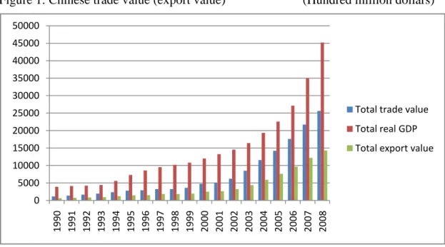
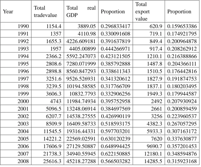
The world economy is steadily moving towards to the integration, any country or region will inevitably be subject to the influence from other nations or regions, especially in China (Shah 2010). According to Ministry of Commerce (see figure 1), the proportion of the export trade dependence rate of Chinese economic has increased to more than 50 per cent in 2008. There is 31.6 per cent of whole country‟s GDP is coming from the export trade (Appendix A1). Meanwhile, the proportion of value both import and export volume of GDP rose from 29.7 per cent in 1990 to 56.25 per cent in the late of 2008. The proportion has doubled in the 20 years. The import and export volume ranking increase from 29th place in 1978 to third place in the late of 2007. China has become a real big trader in the world.
Figure 1: Chinese trade value (export value) (Hundred million dollars)
Source: Ministry of Commerce of China.
0 5000 10000 15000 20000 25000 30000 35000 40000 45000 50000 1990 1991 1992 1993 1994 1995 1996 1997 1998 1999 2000 2001 2002 2003 2004 2005 2006 2007 2008
Total trade value Total real GDP Total export value
4 However, with the U.S. financial crisis‟s effects growing since 2007, it has been getting worse and worse extended to the whole world in 2008. As a main part of the world economic entity, China also cannot avoid the influencing come from the global financial crisis. But compare with the U.S., the main European countries and other developing countries, the effects to China are smaller. According to the Shah (2010), the main influence reflects on the negative growth of export, slow down the investment growth come from the foreign companies and devaluation of the foreign exchange assets of China.
According to the statistics of the U.S. Department of Commerce end of 2007, China is the second largest trade partner and has exceeded Japan became the third export market of the U.S.; meanwhile became the first import market of the U.S. after exceeded Canada in 2007. From the point of view of trade dependence, the dependency ratio of the China-U.S. trade in recent year rising from 5.4 per cent in 1997 to 9.76 per cent in 2006, and amounted to 8.95 per cent in 2007, China‟s export trade has gradually become a dependency on the U.S. market. Thus, the high degree of dependence on the U.S. market, the volatility of the U.S. economic market has a greater impact on China‟s export trade. According to the statistics in the beginning of 2008 by the U.S. Department of Commerce, it is shown that the U.S. trade deficit fell to 16.1 billion dollars, a decrease of 12.4 per cent to its lowest level in around two years. Among them, the export of China to U.S. has decreased 7 percent.
At the same time, in the recent 30 years, in order to make up the shortage of fund, technology, equipment and management, China used more foreign investment to develop and got remarkable effects. According to the statistic comes from the Ministry of Commerce of China and Invest in China, from 1979 to 2007, the foreign investment capital which China directly used is about 760.2 billion dollars. It is about 26.2 billion dollars per year; the use of foreign capital has been living in the world's top three since 2002. At the end of 2010, the foreign direct investment has been
5 achieved 114.73 billion of dollars. There is the statistic for resenting year accorded to the Invest in China from 2003 to 2010:
Table1: The foreign direct investment in China (Billion dollars)
Year FDI Increase proportion
2003 53.505 1.44% 2004 60.63 13.32% 2005 72.406 19.42% 2006 69.468 -4.06% 2007 79.075 13.83% 2008 108.312 29.70% 2009 94.065 -13.20% 2010 114.73 22%
Source: Invest in China
In the table above shows that in 2009, the FDI even had a negative growth rate about 13.20 percent. The foreign investment is a main part of Chinese export trade and China‟s developing. So when the economic entities of the U.S. and other foreign countries are affected by the financial crisis badly, they reduce the investment in China, which directly influence the volume of Chinese export.
In the period of the U.S. financial crisis, the international financial market instability, the growth rate of world economic decrease a lot, the change of the external economic environment also took impact on the Chinese export. From November of 2008, the real value growth rate has become negative and decease by 2.2 per cent (accorded to Appendix A3), it is the first time has a negative growing. Because the shortages of market liquidity, the investment and consumption confidences have been hit badly, so the foreign consumer demand for both high value-added products and low value-added products all decease a lot. The EU, the U.S. and Japan are China‟s top
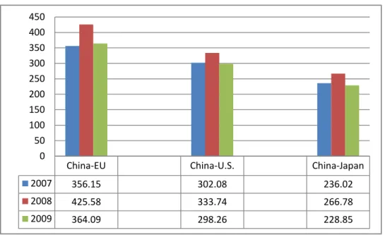
6 three trading partners, affected by the financial crisis; export growth rate to the three markets have come down obviously in 2008 and 2009 (accorded to AppendixA2) and showing in table 3. With the China‟s major trading partners, the European Union is still the biggest one, American and Japan followed. According to General Administration of Customs of China, in the year 2007 to 2009, the top three partners‟ bilateral trade value (both export and import) like following in Figure 2:
Figure 2: Bilateral trade value (Billion dollars)
Source: General Administration of Customs of China
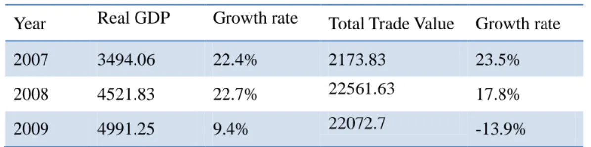
Meanwhile, due to the U.S., Europe and Japan, the economic downturn caused by the financial crisis will inevitably lead reduce in demand. According to IMF statistics, with the continual effect of the financial crisis, in 2009, the global economic growth continued to fall by 1.5 percentage points; the U.S. economy falls 0.7 per cent and the Euro area decreased by 0.5 per cent. In addition, world trade growth increased by 2.1 percent in 2009. However there still has 2.5 per cent decline compared with 2008. In this context, China‟s exports also are greatly affected. In 2009, the real GDP and the total trade value of China all had a big decrease in growth rate.
As follows in table 2 shows:
China-EU China-U.S. China-Japan 2007 356.15 302.08 236.02 2008 425.58 333.74 266.78 2009 364.09 298.26 228.85 0 50 100 150 200 250 300 350 400 450
7 Table 2: Chinese real GDP and total trade value (Billion dollars) Year Real GDP Growth rate Total Trade Value Growth rate
2007 3494.06 22.4% 2173.83 23.5%
2008 4521.83 22.7% 22561.63 17.8%
2009 4991.25 9.4% 22072.7 -13.9%
Source: Ministry of Commerce of China.
Due to the previous overview of the Chinese trade we can see China is the country rely on export-led economic growth and have a tight connection with international economics and trade, Tai Wan and Hong Kong are the first export-led economic growth areas in the early 1960s and 1970s, accorded to Seck (2009). The economic growing condition is highly dependent on the export trade growth, when the external environment is affected by the global financial crisis; it will also have a negative impact to the Chinese export. This thesis will estimate the effect come from the financial crisis on Chinese export by using gravity model, so the following part will be the theoretical framework of this thesis, the gravity model. And then in part 4will review the previous literatures which relate to the export-led economic growth policies economies and global financial crisis.
8
3. Theoretical framework- Gravity model
According to Liu, Huo and Chen (2011), most of the empirical analyses of influencing factors in the export or bilateral trade research are based on the gravity model. The trade gravity model is coming from the classical gravity model of Newton, the Newton‟s universal law of gravitation in physics that the gravitational attraction between two objects is proportional of their masses and inversely relates to distance‟s square. The model is expressed as follows:
Fij=MDiMj
ij2 (1)
Where:
Fij is the gravitational attraction Mi, Mj are the mass of two objects
Dij is the distance
The famous econometrician Tinbergen used the gravity model to explain international bilateral trade in 1962 (cited in Krugman and Maurice, 2005). The model applied in the bilateral trade useTij as the total trade flow from origin country „i‟ to destination
country „j‟ instead of Fij. Yi and Yj are the economic size of the two country „i‟ and
„j‟, the Yi, Yj are always use GDP of two countries. The „Dij‟ is also the distance between two countries. Always use the distance of two capital cities, according to Krugman and Maurice (2005). The model just like following:
Tij= AYDiYj
ij (2)
Tinbergen‟s study results show that, the flows of trade between two countries depend largely on the scales of two countries size base on GDP and the distances of the geopolitical, meanwhile, the longer the distance, the less the trade flows.
9 Although the gravity model was used well in analyzing the international trade flows in the 1960s, like econometrician Tinbergen, the theoretical foundations were not produced until 1970s. James E, Anderson (1979) (cited in Liu, Huo and Chen, 2011) maybe the first who mentioned the theoretical basis for the gravity models. He indicated when the economics of scale are certain; the volume of trade will be reduced because of the bilateral trade barriers between two countries.
The gravity model is also used to estimate the bilateral trade value. Ma and Cheng (2003) used the gravity model to estimate the theoretical predictions. The main idea is that the trade between a pair of countries is positively related to the sizes of the economies, like GDP, GNP, and negatively related to the distance between the countries. Besides, in their paper also has shown that the imports and exports will fall due to the financial crisis in 1991-1998 with 50 countries data.
However, the equation (2) is too simple to estimate the real world situations. The geographical size, population and openness to trade are also the important factors which affecting exports and import trade. Thus, just like Eita stated in his paper, in the general form to the gravity modal, the exports from country i to country j are determined by their economic sizes (GDP), population, geographical distances and dummy variables, it is generally specified as follows (Martinez-Zarzoso and Nowak-Lehmann, 2003: 296; Jakab, Kovacs and Oszlay, 2001: 280; Breusch and Egger, 1999: 83):
𝑋𝑖𝑗=𝛽0𝑌𝑖𝛽1𝑌
𝑗𝛽2𝑁𝑖𝛽3𝑁𝑗𝛽4𝐷𝑖𝑗𝛽5𝐴𝑖𝑗𝛽6𝑢𝑖𝑗 (3)
Where 𝑋𝑖𝑗 is the exports of goods from country i to country j, 𝑌𝑖 and 𝑌𝑗 are the GDP of the exporter and importer, 𝑁𝑖 and 𝑁𝑗 are the populations of the exporter and importer, 𝐷𝑖𝑗 is the distance between two countries, 𝐴𝑖𝑗 is other factors which influence trade between two countries and the 𝑢𝑖𝑗 is the error term.
10
4. Literature review
4.1 Export-led economic growth policies economies
According to Adam and Chua (2009), Asia‟s developing economics are almost twice as reliant on exports as the rest of the world, with 60 percent of their overseas sales ultimately destined for the U.S., Europe and Japan. Since the 1960s to 1970s, the four Asian tiger economies like Singapore, Taiwan, South Korea and Hong Kong had a huge economic development relied on the export-led economic growth model. They exported big quantities of goods to the U.S., Europe and other First World countries by which made them achieved First World standards of living. Although the New York University economics professor Nouriel Roubini has declared the Asian export-led growth model turns out to be broken, because in the times of the financial crisis, the nations of the Asian need to increase their domestic consumption in order to make up for the fall in U.S. imports, the idea also seems impractical, accorded to Seck (2009).
Babatunde and Busari (2009) also mentioned in their studies, the export-led growth hypothesis is one of the main determinants of growth of Africa; meanwhile, the growth of national income per capita remained unstable (Hammouda, 2004). However, in the times of the 2008 financial crisis, the slowdown of the Africa‟s economic has shown that export-led growth could make fragile economies very vulnerable and led to major negative volatility, when they studied the export-led growth model for Africa.
Meanwhile, for the developing export-led economic growth countries always consist mainly two tradable sectors which are the manufacturing and agriculture, according to Meyn and Kennan (2009), “the fuel and mining products are highly responsive to global gross domestic product changes and the agricultural products are generally income inelastic.” They analyzed the effect comes from the financial crisis on trading prices and volumes from different composition of their export products. Many
11 developing countries depend on export few commodities for the bulk of their export revenue. Then the elasticity of the commodity‟s demand in the importing country is the essential element of how an economic crisis affects their export revenue. Most of the exporting countries are depending on agricultures exporting like China, Mexico and fuel exporting like the West Asian countries. The products like fuel is fixed in the short run, the oversupply will depress the price in the future, but the agricultures like tea and crops are basic necessity goods, they lower income elasticity of demand.
According to AFDB (2004), the traditional agricultural exporters also have diversified into non-traditional agricultural exports, like fresh vegetables and special fruits which not produced by domestic, are generally less affected by volatility in terms of trade. However just like Barichello (1999) has shown that the Asian crisis resulted in reducing demand for coffee, rice, sugar, tea and so on. Because in times of crisis the income elasticity for these non-traditional agricultural items are higher than for basic crops and they are likely to be substituted by domestic goods. And the deeper the crisis, the more likely it is that traditional agricultural products will also be affected by decreasing demand.
Manufactured goods are also the characteristics of the developing exporter country, such as the clothes and electronics; they also show an income elasticity of demand. Many Southeast Asian countries depend on exporting simple manufactures for the bulk of their export revenue. But there also have risks as discussed by the UN Conference on Trade and Development (2002), the developing export countries with large supply capacities are able to produce labour-intensive products at lower cost than other countries. So at the time of crisis, importing countries will prefer to use less money to buy more goods, the big export countries will show their advantage, like China, the biggest export developing country.
In recent studies, like Meyn and Kennan (2009) expressed the financial crisis affects developing country manufactured exports not only because of the high income
12 elasticity of demand for manufactured products but also because of their high dependency on imported inputs. About ten years ago, in the times of Asian crisis, Boorman et al. (2000) stated the sourcing of inputs for manufactured exports might be severely constrained by depreciated currencies and restrictive trade finance conditions, like the Southeast Asian exports of computer during the Asian crisis in 1997.
Mexico also is an export-led economic growth country, Villarreal (2010) stated that Mexico had experienced the deepest recession in the Latin America region just because the 2008 global financial crisis, due to its high dependence on manufacturing exports to the U.S. The real GDP of Mexico even got the negative 6.6 percent in 2009. In 2009, the Mexico‟s total trade with the world declined sharply with lower demand in the U.S. for Mexican products and lower consumer demand in Mexico contributing to the decline.
There also have a different basis for export-led growth offered by Feder (1983); the exports are as an explanatory variable in a traditional growth framework with a production function. In Feder‟s model, the output of the non-export sector depends not only on the factors of production the labour and capital and also on exports. This captures the externality associated with factors unique to exports such as higher-quality labour and internationally competitive management.
Previous literature reviews illustrate that many developing countries have attempted to pursue the East Asian growth model, and have become an export-led economic growth country. But under the global financial crisis, the crisis also brings obvious effect on these fast growing countries‟ economies. China as the biggest developing country in Asian also is an export-led economic growth country, after accession to the WTO, it has allowed China to fully integrate into the world system and capture the gains of its comparative advantage in abundant labour supply (Yao, 2011). From the literature review, there have effects come from the financial crisis on the export-led economic growth economic entries. In the following part, there will review the effects
13 come from the financial crisis on the countries of the world.
4.2 Global financial crisis and its effects
Back to 25 years ago, the „Black Monday‟ in the October 19, 1987 was known as the largest one day drop in the history of the New York Stock Exchange Market. It caused the Wall Street to crash and then began the depression for the whole country. According to Michel (1997), in the 1987, 22.6 percent of the value of the American stock was decreased in the first hour in the Monday morning. It was also given a big effect on the European and Asian stock market through the financial system.
Almost 10years later, July 2, 1997, the Asian financial crisis was started, Ed (2009) has concerned the Thai Baht was the first currency to experience problems. In that day, the exchange rate of Thai Baht for dollar decrease by17 percent, the foreign exchange and other financial markets got into a mess. In the following months, all the Asian countries‟ stock markets were shocked by the crisis. In the August 15, 1997, the Wall Street also suffered its worst day since 1987; the Dow Jones dropped 247 points. The tumble on August 15 also immediately spilled over to the world‟s stock markets, Hong Kong, Tokyo and European exchanges.
The first major financial crisis of the 21st century as well as the newest one is the U.S. sub-prime mortgage financial crisis, Carmen and Kenneth (2008) said. According to Lucjan (2008), the crisis has five stages, the beginning is the housing bubble in the U.S. increases the inflated by subprime mortgage lending and then spread into other types of assets like investment banks. And the third important effect is that it turns into the global liquidity crisis when the lots pullout of liabilities from the banks, like Lehman Brothers, spread into the global scale. Fourth, the collapse of collateralised debt obligations which also caused the bubble effects in the commodity futures market. Finally, lots of fund shifts in risk-free securities, the Lehman Brothers filed for bankruptcy protection the whole U.S. investment banking system crashed. The
14 whole world was alarmed by the bankruptcy of Lehman Brothers and also alarmed by the U.S. financial crisis.
Just like Shah (2008) said, the global financial meltdown will affect the livelihoods of almost everyone in an increasingly interconnected world, the crisis not only affect one country‟s people also affect the livelihoods of others. Eichengreen, Rose and Wyplosz (1997) used the Probit model to estimate about 20 industry countries to see the probabilities of a financial crisis occur. The result indicated that the financial crisis is easier to spread between the counties with the trade connections. Nearly every country in the world has the trade connection, that's why the crisis can always affect in a big scope. Masson (1998) also confirmed this point, as under the environment of integration with the global economy, the commodity trade is the main channel for financial crisis spread. Coughlin and Pollard (2000) estimated how much the financial crisis affects the different countries, found that the countries rely on the Asian countries‟ export have had the worst influences. Through Fernald, Edition and Loungani (1999) studies, the Asian crisis made the export of China decreasing badly, because the financial crisis made the other Asian countries‟ needs of import decreased so much. Niu, li and lai (2000) also said that, when the counties have the financial crisis, the import needs will decrease which will cause China‟s export decrease.
According to Gunawardana (2005) research result I can see that under the influence of the Asian financial crisis, Australian‟s export to the other nine Asian countries has the positive correlation with the nine counties‟ real GDP and GDP per population, and the negative correlation with the real exchange rate when the rate following down. Mckibbinand Stoeckel (2009) in their study said the U.S. is a large importer of China, as a matter of fact, the export of China will fall as import of U.S. fall, with a combined effect from the three shocks, a drop in GDP, stock market value and consumption.
15 No matter the developed countries or the developing world, the financial crisis all gave a big hit for their GDP growing even gave a negative growing. In the developed world, among members of the Organization for Economic Cooperation &the Development (OECD), the GDP grew by just 0.2 per cent in quarter 2 2008, down from 0.5 per cent in the first quarter of the year, according to OECD estimates.
As the Chandy, Gertz, and Linn (2009) reports stated at the outlook come from IMF, because the crisis, the global output has negative 1.3 per cent growth, in the U.S., there has 2.8 per cent negative growth and Germany with 5.6 per cent negative growth. The worst negative growth countries are Japan and Russia which with 6.2 per cent and 6.0 per cent negative growth rate respectively. Only China and India had positive growth in 2009, but Yu (2010) also stated at the end of 2008, China‟s GDP growth rate dropped to 6.8 per cent in the fourth quarter from the 13 per cent in 2007, and did not have a better change in 2009.
Meanwhile, until now, the gravity model has widely used in the international trade in the world, also has been used in estimating the trade potential. Like De (2009), his approach is to estimate trade potential between India and its partner countries using the basic gravity mode. Kwack et al. (2007) used 30 countries‟ sample panel data for the analysis the relationship between the exports and other variable which can affect the export through the gravity model. Jiang (2004) and Jin, Wan and Zhang (2011), all use the gravity model to analysis the export of Vietnam and China which affect by the financial crisis. The dependent variables are like GDP, populations, distance and economic variables like the exchange rate between two countries.
Previous studies have shown that the effect of global financial crisis was reflected directly on the export or import between different countries in the world scale. The influences come from financial crisis were reflected in the GDP, stock market price and unemployment economic indexes etc. Meanwhile these economic indexes are also having internal relations, they are influencing each other. Although there are so
16 many studies and results come from the previous experts, but most of them are regarding to the Asian financial crisis in 1997, and the results are little bit scattered. And a few studies about the new global financial crisis started in 2007 the American financial crisis, especially the effects of this crisis on the Chinese economy, the export come from China to the U.S., EU and Asian countries. So the thesis will do the research in the times of the 2007 global financial crisis, to see the effects of global financial crisis on Chinese export by using past data. And the model be used is the gravity model.
In the empirical framework part, I present the empirical framework of the thesis. Through so many previous empirical estimations of gravity model, we can find that the gravity model is applied to study the bilateral trade; the dependent variable of the gravity equation is always being the trade variables. Just like I have mentioned through the theory of literature reviews, in this thesis I will choose Chinese export volumes as the main trade variable, using the gravity model for analysis the effects of financial crisis on Chinese export to other countries. China will be the exporter, and ten main importers which also under the effect come from financial crisis in 2007-2010, by using the gravity model and panel data models for analysis.
17
5. Empirical Frameworks
5.1 Modeling
The gravity model specification similar to Newton‟s law as following:
𝑇𝑖𝑗= A𝑌𝑖𝛼𝑌𝑗𝛽𝐷𝑖𝑗−𝛾 (4)
A is a constant term, Tij is the total trade flow or exports from i to j, Yi and Yj are the economic size, gross domestic product or gross national product and the economic mass like population. And Dij is the distance between two countries, in this model always treats as the trade cost. In order to do the linear regression analysis, I transform the equation (4) into natural logarithm form; the linear model with a double - logarithm form can make the elasticity of the function constant, so I got the equation like:
𝑙𝑛𝑇𝑖𝑗 = A + 𝛼𝑙𝑛Yi+ 𝛽𝑙𝑛Yj –𝛾𝑙𝑛Dij (5)
Meanwhile, according to the theory of the general gravity model which mentioned by Martinez-Zarzoso et al.; for the exports between exporter and importer, the model I build is basically relied on the gravity model for this thesis:
𝑋𝑖𝑗𝑡=𝛽0𝑌𝑖𝑡𝛽1𝑌
𝑗𝑡𝛽2𝑁𝑖𝑡𝛽3𝑁𝑗𝑡𝛽4𝐷𝑖𝑠𝑖𝑗𝛽5 (6)
I also change the equation in log form for the purpose of estimation and add the dummy variable and error term. Get the estimated gravity model as follows:
L𝑛 Xijt = β0 +β1L𝑛(Yit) +β2L𝑛(Yjt) +β3L𝑛(Nit) +β4L𝑛(Njt) +β5L𝑛 (Disij) +
18 t: time period of sample data.
i: exporter country (China). j: export destination countries.
Xijt: The export volume from China to country j in the time t.
Yit: Chinese GDP in time t. Yjt: Country j GDP in time t.
Nit: Population of China in time t.
Njt: Population of country j in time t.
Disij: Distance between China and country j.
Dt: The dummy variable (with financial crisis or not, Dt= 1, period of financial crisis;
Dt= 0, otherwise).
εt: Error term.
5.2 Data
In the economic model, the GDP is usually measured as the real gross domestic product of the origin countries. So in this thesis I use the real GDP of these countries. Meanwhile, the export volumes from China to the ten export destination also will be the real export value of China. The data of real value of China to import countries are coming from the website of the Customs Bureau of Ministry of Commerce of China. And the real GDP and population of countries are all come from the website of The World Bank. The data of distance between two countries are coming from the website of Distance Calculation Org.
The dependent variable in the current empirical study is the real value of Chinese export to its major export destinations. The data come from the website of the Customs Bureau of Ministry of Commerce of the China during the sample period of 2001 to 2010.
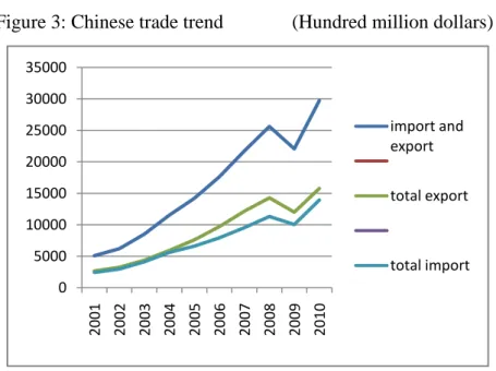
19 According to Customs Bureau of Ministry of Commerce of the China, the statistic was published in 2011, from the year 2001 to 2007, the exports of China were having constantly increasing rate around 30 per cent, there even have 35.39 per cent at the end of the year 2004, and the lowest is also getting 22.36 per cent at the end of year 2002. But in the middle of the year 2007, the USA financial crisis started in the U.S. and has become the global financial crisis in 2008. At the same time, at the end of 2008, the exports and imports growing rates all had obviously declined. The rates decreased by 8 per cent at the end of the year 2008, and even had a negative growth rate in the following year, at the end of 2009 when also the period global financial crisis had affected the whole world deeply and till to 2010. After the collection and statistic, get the following figure as below:
Figure 3: Chinese trade trend (Hundred million dollars)
Source: Customs Bureau of Ministry of Commerce of the China
The figure shows that there has the decrease both in export and import from China at the beginning of 2008 and got even worse in the middle of 2009. As the obviously information as we can see from the chart, the values of the vertical axis is the actual trade value for the each year (unit: hundred million dollars). When the global financial crisis comes, there also have a huge decrease in the trade of China‟s import and export; so the period I choose from 2001 to 2010, ten years to estimate the China‟s export in
0 5000 10000 15000 20000 25000 30000 35000 2001 2002 2003 2004 2005 2006 2007 2008 2009 2010 import and export total export total import
20 the context of global financial crisis.
According to Customs Bureau of Ministry of Commerce of the China‟s statistic, there are 232 countries are the Chinese export destination countries.
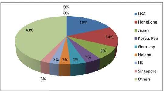
Figure 4: Chinese export major destinations
Source: Customs Bureau of Ministry of Commerce of the China
From the figure 4, we can see the ten major export destination regions USA, Hong Kong, Japan, Korea, Germany, Netherland, UK, Singapore, India and Italy from China have taken 60 per cent of the total Chinese exports. These countries were also influenced by the financial crisis badly shock in the 2007-2010. Table 3 below shoes descriptive statistics of the Chinese export to the ten major destinations:
Table 3: Descriptive Statistics (Billion dollars) Export
value
Minimum Maximum Median Standard
deviation Mean U.S. 54.28 283.29 183.17 80.79 169.71 Hong Kong 46.55 218.30 139.89 59.82 132.16 Japan 44.96 121.04 87.80 26.84 83.90 Korea, Rep. 12.52 73.93 39.82 22.01 40.81 Germany 9.75 68.05 36.42 20.39 36.11 Netherlands 7.28 49.70 28.37 15.44 27.89 UK 6.78 38.77 21.57 11.89 22.15 18% 14% 8% 4% 4% 3% 3% 3% 43% 0% 0% USA HongKong Japan Korea, Rep Germany Holand UK Singapore Others
21
Singapore 5.79 32.35 19.91 10.89 19.85
India 1.90 40.91 11.76 14.15 16.35
Italy 3.99 31.14 13.83 9.43 15.15
Before running estimation, as shown in table 4 below the expected signs for each variable‟s coefficient can be summarized as shown in table 4 below:
Table 4: Expected signs
Variables Expected signs
𝐘𝐢𝐭 Positive
𝐘𝐣𝐭 Positive
𝐍𝐢𝐭 Either positive or negative
𝐍𝐣𝐭 Either positive or negative
𝐃𝐢𝐬𝐢𝐣 Negative
𝐃𝐭 Negative
When the national income increases, people will have more available money to buy the commodities. So the importing country with a high level of income in will have high imports, the signs of 𝛽1 and 𝛽2 are expected to be positive in equation (7).
The coefficients of 𝛽3 and 𝛽4are for the population of the exporting country (here is China) and the importer countries cannot be expected in advance. It can positive or negative, according to Martinez-Matzos and Nowak-Lehman (2003), a large population will be having a large domestic market and higher degree of self-sufficiency and less trade demands. Large populations also have variety of labour and this means there is economics of scale in production, and opportunities to trade in a variety of goods, then the coefficient for populations will be negative. On the other hand, large population has large domestic market and labour can create large opportunities for trade in more variety of goods. In this case, the sign of coefficient will be positive. It depends on whether the export country exports more when the
22 population is large and also depends on whether the import country imports more when the population is small.
The distance variable relates to the transportation cost between China and the import countries, the main export port in China is not the capital Beijing, is in the north part of China, Guangdong province. The Guangdong‟s export volume ranks first in China and made large contributions to the country‟s foreign trade. So Guangdong is chosen as the export center from China to calculate the distance to the five import countries‟ capital cities where is measured as the minimum distance along the surface of the earth. The distance variable is expected to have a negative effect of trade because the longer will be the larger to the transport cost. So the sign of coefficient 𝛽5 will be
expected to be negative.
There also has the dummy variable for the global financial crisis come from USA in beginning in the middle of 2007 till 2010, in order to study the effects of the financial crisis effect on Chinese export. As I have mentioned above the statistic data also clear shown the Chinese trade have declined during the period of global financial crisis, so the coefficient of the dummy variable 𝛽6 is expected to be negative.
23
6. Empirical findings
6.1 Unit root test
According to the principle of statistics, if the time series is not stationary, then the result will not reflect the real relationship between the dependent variables and the independent variable, and the regression will also become to spurious regression. Due to the data is the annually in the period from 2001 to 2010 in ten countries and I will use panel data model, avoiding getting the spurious regression, I need do the unit root test for my sample data.1,2 Therefore, the unit root test was done for individual series variables. The results of the ADF test for unit root are shown in tables:
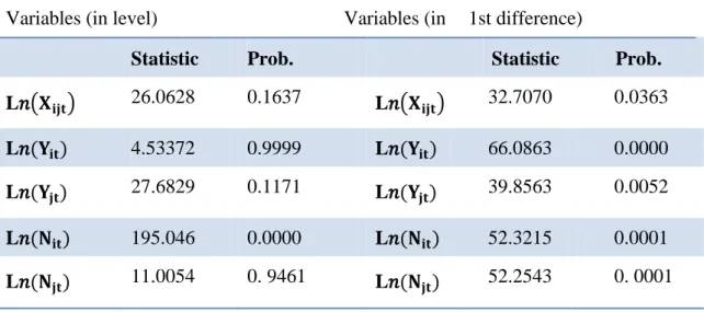
Table 5: Test for unit roots in Levels and first difference:
Variables (in level) Variables (in 1st difference)
Statistic Prob. Statistic Prob.
L𝑛 𝐗𝐢𝐣𝐭 26.0628 0.1637 L𝑛 𝐗𝐢𝐣𝐭 32.7070 0.0363 L𝑛(𝐘𝐢𝐭) 4.53372 0.9999 L𝑛(𝐘𝐢𝐭) 66.0863 0.0000 L𝑛(𝐘𝐣𝐭) 27.6829 0.1171 L𝑛(𝐘𝐣𝐭) 39.8563 0.0052 L𝑛(𝐍𝐢𝐭) 195.046 0.0000 L𝑛(𝐍𝐢𝐭) 52.3215 0.0001 L𝑛(𝐍𝐣𝐭) 11.0054 0. 9461 L𝑛(𝐍𝐣𝐭) 52.2543 0. 0001 1
Due to the limitation for my data collection, my data‟s sample size is small, both T (time period) and N (countries number) are all equal to 10. But the DF distribution for the critical values was based on the sample size of 25 in the smallest sample size. The degrees of freedom are small and thus would be inaccurate in this case.
2
The common testing for unit roots in panel data are LL test suggested by Levin and Lin (1992, 1993) and IPS test suggested by Im, Pesaran and Shin (1997). However, when the sample data‟s N and T are relatively small (normally the number of N should from 10 to 250 and the T from 25 to 250), the panel unit root tests do not provide clear-cut results.
24 So from the forms shown, the time series of variables L𝑛(Nit)in level is stationary,
but the variables are all stationary at first-difference.
According to all the variables are the first differences stable for the time series unit root test except the L𝑛(Nit). In the real economic problems, the data‟s time series are always non-stable, we can make the difference process to make them stationary. First-difference of the variables in the logs has an interpretation of growth rates. Therefore, first-differenced series are used in estimation.
25
6.2 Estimation results
3For the panel data models, there are two ways to estimate, the fixed effects and the random effects (Verbeek, 2007). In order to choose between the models, I use the Hausman Test, the general idea of Hausman test is to compare two estimators which one is consistent under the null (Ho:𝑥𝑖𝑡 and 𝛼𝑖 are uncorrelated) and an alternative hypothesis and the other is only consistent under the null hypothesis. If the difference between the two estimators is significant, then we can reject the null hypothesis.
But for the gravity model, one of the short comings of the fixed effect model is that it cannot identify the impact of time invariant, such like distance between two countries. But the distance is an important variable in my paper. Penh (2008) in his study also stated the disadvantage for the fixed effect model, it cannot estimate coefficient for distance, common language and so on. So first I run the estimate by random effects in Eviews, and then do the Fixed/Random effects testing; Hausman Test of which result is the following:
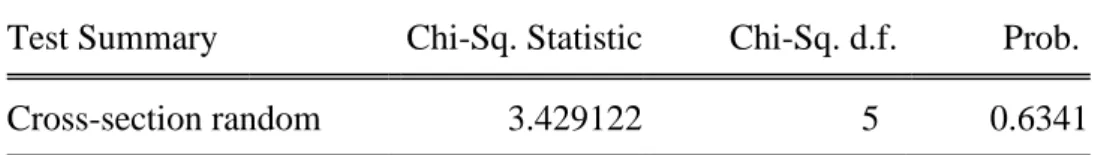
Table 6: Hausman Test result
Correlated Random Effects - Hausman Test Test cross-section random effects
Test Summary Chi-Sq. Statistic Chi-Sq. d.f. Prob.
Cross-section random 3.429122 5 0.6341
From the result of the Hausman test, we cannot reject the hull hypothesis that I will choose the Random effects model. Built my interpretations of results based on the Random effects model. In order to use the stable data, the data of the time series
3
The estimation results presented here are based on using the top 10 Chinese export destinations. However, due to the small sample size problem that was mentioned earlier, estimation was done by including 10 additional Chinese export destinations (See appendix table A11). The dummy variable for the crisis period is not statistically significant in case of using the top 20 export destinations.
26 variable all have changed into first difference. And then I got the results as follows in the table:
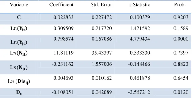
Table 7: Estimation results
Variable Coefficient Std. Error t-Statistic Prob.
C 0.022833 0.227472 0.100379 0.9203 L𝑛(𝐘𝐢𝐭) 0.309509 0.217720 1.421592 0.1589 L𝑛(𝐘𝐣𝐭) 0.798574 0.167086 4.779434 0.0000 L𝑛(𝐍𝐢𝐭) 11.81119 35.43397 0.333330 0.7397 L𝑛(𝐍𝐣𝐭) -0.231162 1.557006 -0.148466 0.8823 L𝑛 (𝐃𝐢𝐬𝐢𝐣) 0.004693 0.010162 0.461878 0.6454 𝐃𝐭 -0.108051 0.042089 -2.567212 0.0120
R2= 0.458787 ; Adj. R2= 0.419664, and F-statistic 11.72655.
The full random effects model results are also shown in Appendix table A10. Due to the results, the average intercept value of the regression model is 0.022833. Although there has the limitation for example data collection, but the time series data all got through the unit root test and shown are all stationary in first-difference. Meanwhile through the Hausman test, the estimation results come from the random effects model are reliable and unbiased. So the following discussion will base on the results as shown above.
27
6.3 Discussion of the Estimation Results
When estimating the regression model, all the time series variables use the first-differenced data, so the variable L𝑛(𝐘𝐢𝐭) means the real GDP growth rate of
China, L𝑛(𝐘𝐣𝐭) means the real GDP growth rate of the export destination countries,
L𝑛 (𝐍𝐢𝐭) means the population growth rate of China and the L𝑛 (𝐍𝐣𝐭) is the population growth rate of export destination countries.
The coefficient estimates of the real GDP growth rate of Chinese export to destination economies and the dummy variable for the financial crisis. The R2 of the linear regression function is 0.458787 meaning that 45.88% of the variance of the dependent variable about its mean can be explained by the regression model. The export of China is relatively affected by the real GDP growth rate of export destination countries and whether there have financial crisis or not.
According to previous studies, when one country‟s real GDP is higher or the GDP has positive growth rate, the import of the country will also increase, so that it will increase the export of China. So when I build my regression model for Chinese export, the real GDP of the export destination country or the real GDP growth rate is expected to have a positive effect on Chinese export. The coefficient of the real GDP growth rate of export destination countries is +0.798574, the sign of coefficient matches my expectation which is positive. It means when the real GDP of export destination countries increases one per cent, the export growth rate of China will increase 0.798574 percent, and the P-value is 0.0000 which is significant in the model. It means with the impact of global financial crisis, the real GDP growth rate of these ten countries decreases or decrease in real GDP, will impact the import of these ten countries. Meanwhile, this will affect the Chinese export and the Chinese export growth rate.
28 And for the dummy variable, if the year have global financial crisis, the value will be 1, otherwise will be valued 0. According to the result, the sign of the coefficient for dummy variable is negative as expected, the coefficient estimate is -0.108051. It states that in crisis periods, Chinese export growth rate decreases by 11.4105 per cent, where 11.4105% comes from [(exp (0.108051) -1) *100%]. P-value is 0.0120 meaning that the coefficient estimate is statistically significant in the linear regression model.
The coefficient estimates of export destination economies‟ real GDP growth rate and the dummy variable are statistically significant while those of other variables are statistically insignificant. Although they are statistically insignificant, discuss signs of the coefficient estimates is still meaningful. For the variable Chinese real GDP growth rate, the sign of coefficient is also matched my expectation which is positive, China is a big exporting country, when the real GDP is higher will also let the export value higher. The coefficient is +0.309509 means an increasing of the real GDP growth rate of China one per cent, the Chinese export growth rate will increase 0.309509 percent. But the P-value is 0.1589 which cannot reject the null hypothesis so that the GDP of China is insignificant for the estimated regression model.
For the populations both China and its export destination countries, as I have mentioned the sign of coefficient cannot be expected in advance. From the estimation results we can see the sign of population of China growth rate is positive and the coefficient is 11.81119, which means when the population of China growth rate increase one per cent, the growth rate of Chinese export will increase 11.81119. This maybe because China is an export country and there have so many employees working for export companies. But the P-value is 0.7397 cannot reject the null hypothesis so that the variable is statistically insignificant. And for the variation of population growth rate of export destination countries, the coefficient is -0.231162, the sign is negative. It means when the import country‟s population growth rate increase one per cent, the growth rate of Chinese export will decrease 0.231162
29 percent. And the P-value is 0.8823 cannot reject the null hypothesis so that the variable has also been statistically insignificant. This happens maybe when the population growing in the importing countries, they will have a large domestic market and higher degree of self-sufficiency and less trade demands, accorded to Martinez-Marzoso and Nowak-Lehman (2003).
The distance variable measures the transportation cost between two places, the longer distance will the larger transportation cost. The sign of the coefficient is also matched my expectation which is negative. But the coefficient of the variable in my mode is 0.004693; it is positive and does not match my expectation which should be negative. It means when the distance of two places increase one per cent, the export growth rate of China will increase 0.004693 percent. However, as I have mentioned above, the America and Europe are the main places of Chinese export destination, the distances are much longer than other economies of China, in recent years, the transportation will also not cost too much, that is why there have a positive sign in the distance in my model. Meanwhile the absolute value is 0.004693 which is really small and p-value of distance is 0.6454. Thus we cannot reject the null hypothesis. This variable is statistically insignificant for the linear regression model.
From the results of the estimation, the absolute value of the coefficient of population growth rate of China is 11.81119, it is really a high value which because China with abundant labour supply so that with the growth rate increase also increase the Chinese export growth rate. And the absolute value of the coefficient of GDP growth rate of export destination countries is 0.798574, and the statistic value p with high significance. It is shown that with the impact of global financial crisis, the growth of GDP of export destination countries decreases, obviously slow down the speed of the export growth rate of China. And the less effect comes from the real GDP growth rate of China and the population growth rate of importing countries, the values are 0.309509 and 0.231162. Finally, the last effects are coming from the distances
30 between China and ten import countries and the dummy variable, the value are 0.004693 and 0.108051 respectively.
31
7. Conclusions
This thesis has shown the global financial crisis impacted economic conditions of the main economies like the U.S., Japan and European countries and then effect on Chinese exports. In the empirical model, the dependent variable is the real value of Chinese exports to destination countries, and the independent variables are real GDP and populations of China, real GDP and population of export destination countries, distances between China and export destination countries and the dummy variable.
The focus of this thesis is the exports from China to its major destinations before and after the period of the global financial crisis. Through the statistic description and analysis of the sample data from the period 2001 to 2010 shows that there have effects come from the global financial crisis on Chinese export. The global financial crisis has stroked the ten export destination countries‟ financial market especially national income and hit the confidences of investments and consumptions so that reduce the import demand from abroad. Meanwhile, the ten countries nearly have taken 60 per cent of the total value of Chinese export, so the decrease in import demand of these countries must have influence on export of China. The decrease of real GDP or the growth rate in these countries is the main reason impact of Chinese export. There also have other reasons like the increase of the unemployment rate and decrease of the stock market price all have the negative impact of the Chinese exports. Although with the population growing of these countries they can get more self-sufficiency, it is not the main reason to decrease Chinese export to these countries. So from the thesis, it shows that because of the global financial crisis, the real economy and financial conditions of these countries all have got worse is the main reason affect the decline in Chinese exports.
Financial crisis started from one country spreads to other economies, making it a global financial crisis, the subprime mortgage crisis of U.S. being one of them, have implications on Chinese export as following:
32 First of all, China as a big export country relies on the other countries‟ import demand. China cannot ignore the international market but China can optimize the export structure, meaning that China can upgrade the product structures of export. For example export more products with high technology to win more competitive advantage in the international market. Meanwhile find new target market to decrease the dependence for the difference of country market.
The second point is to make more trade cooperation with other countries. According to The Central People‟s Government of China‟s report (2011), in 2010, China and the ASEAN (The Association of Southeast Asian Nations) Free Trade Agreement is fully implemented, 90 per cent of the goods to achieve zero tariffs, a strong impetus to the rapid growth of China-ASEAN bilateral trade. China attaches great importance to bilateral and regional trade and economic cooperation. The countries and regions signed bilateral trade agreements or economic cooperation agreements with China have more than 150. As of the end of 2010, China has 15 free trade arrangements with 28 countries on five continents and regions. China and other developing countries trade in a more rapid pace of growth in trade with Arab countries, the further development of the field of trade and economic cooperation with Latin American countries also continues to broaden.
The most of the destinations of Chinese export are developed countries with strong powers of economics in the world. So the international economic statuses of these counties have heavily effects of the Chinese economy. China needs to cooperate with them in more different parts, so that decrease the effects of financial crisis on Chinese export can also improve the economic status of China.
33
Reference:
Attri, V. N., (2011), Export-Led Economic Growth in China? New Orleans, Louisiana USA 2011, The 2011 New Orleans International Academic Conference.
Adam, S. and Chua, J., (2008), Singapore's GDP Grows Less Than Estimated; CPI Jumps (Update2), Bloomberg, May 22, 2008 23:16 EDT.
African Development Bank, (2004), African Development Report 2004: Africa in the Global Trading System. Oxford, UK: Oxford University Press.
Babatunde, M. A. and Busari, D. T., (2009), Global Economic Slowdown and the African Continent: Rethinking Export-Led Growth, International Journal of African Studies, Issue 2 (2009), pp.47-73.
Barichello, R. R., (1999), Impact of the Asian Crisis on Trade Flows: A Focus on Indonesia and Agriculture, Farm Foundation, Agricultural and Food Policy Systems Information Workshops, Policy Harmonization and Adjustment in the North American Agricultural and Food Industry; Proceedings of the 5th Agricultural and Food Policy – 1999.
Breusch, F. And Egger, (1999), How Reliable are Estimations of East-West Trade Potentials Based on Cross-section Gravity Analyses, Empirica, 26(2): 81-99
Boorman, J. T., Lane, M., Schulze-Ghattas, A., Bulir, A., Ghosh, J., Hamann, A., Mourmouras and S. Phillips, (2000), Managing Financial Crises: The Experience in East Asia, Working Paper WP/00/107. Washington, DC: IMF.
Chandy, L., Gertz, G. and Linn, J., (2009), Tracking the Global Financial Crisis: An Analysis of the IMF’s World Economic Outlook, Wolfensohn Center for Development at Brookings,May 2009
China’s foreign trade situation report, (2009 spring), Ministry of Commerce of the People‟s Republic of China, September 5, 2009.
Carmen, M. R. and Kenneth, S. R., (2008), Is the 2007 U.S. SUB-PRIME FINANCIAL CRISIS so different? AN INTERNATIONAL HISTORICAL COMPARISON, NATIONAL BUREAU OF ECONOMIC RESEARCH.
Coughlin, C. C. and Pollard, P. S., (2000), State exports and the Asian crisis, Federal Reserve Bank of ST. Louis, January/February 2000.
De, P., (2009), Global economic and financial crisis: India’s trade potential and future prospects, Asia-Pacific Research and Training Network on Trade Working Paper Series, No. 64, May 2009.
34 Egger, P., (2000), A Note on the Proper Econometric Specification of the Gravity Equation, Economic Letters, 66, 25-31.
Ed, V. (2009), 1997 Asian Financial Crisis. Avanti, Improvement Solutions, LLC, Global supply Chain, Process Improvement‟s Papers, 1997 Asian Financial Crisis. Eichengreen, B., Rose, A and Wyplosz, A., (1997), Contagious Currency Crises, NBER WP 5681; CEPR DP 1453, July 1996. Revised March 1997.
Feranld, J., Edison, H. andLoungani, P., (1999), Was China the first domino? Assessing links between China and other Asian economies. Journal of International Money and Finance.
Feder, G., (1983), Journal of Development Economics, On exports and economic growth. 12(1-2):59–73.
Gunawardana, P., (2005), The Asian Currency Crisis and Australian Exports to East Asia, Economic Analysis and Policy (EAP), Queensland University of Technology (QUT), School of Economics and Finance, vol. 35(1-2), pages 73-90, March/Sep. Hammouda, B. H., (2004), Economic Commission for Africa, Trade liberalization and development: lessons for Africa. Africa Trade Policy Centre Work in Progress. Huo, W. D., Liu, T. and Chen, Y., (2011), Study on Guangdong province’ influencing factors of export in the context of financial crisis – Empirical analysis based on 1990-2007 annual data. Paper presented at the 7th Annual APEA Conference, Pusan National University, Busan, Korea.
Im, K. S., Pesaran, M. H., Shin, Y. (1997), Testing for Unit Roots in Heterogenous Panels. Universityof Cambridge, Department of Applied Economics.
Jiang, S. Z., (2004), An Analysis on the Gravity Model of Vietnam's Export and Its Inspirations, All-round Southeast Asia; 2004-11.
Jin, H. F., Wan, L. L. and Zhang, C., (2011), the effects of financial crisis on Chinese exports trade, Financial Trade, F832.
Jakab, Z. M., Kovacs, M. A. andOszlay, A., (2001), How Far has Regional Integration Advanced?: An Analysis of the Actual and Potential Trade of Three Central and European Countries, Journal of Comparative Economics, 29, 276-292. Krugman, P.R., and Maurice, O., (2005), International economics: theory and policy, 7.ed, Boston, Addison-Wesley.
Kwack S. Y., C. Y. Ahn, Y. S. and Lee, D. Y. Yang, (2007), Consistent Estimates of World Trade Elasticities and an Application to the Effects of Chinese[J]. Journal of Asian Economics, 18, 314-330.
35 Lucjan, T. O., (2008), Stages of the Ongoing Global Financial Crisis: Is There a Wandering Asset Bubble?, IWH Discussion Papers 11, Halle Institute for Economic Research.
Levin, A., Lin, C. F. (1992), Unit Root Tests in Panel Data: Asymptotic and Finite Sample Properties. University of San California, San Diego, Discussion Paper No: 92-93.
Levin, A., Lin, C. F. (1993), Unit Root Test in Panel Data: New Results. University of San California, San Diego, Discussion Paper No: 93-56.
Ma, Z. H. and Cheng, L. K., (2003), The effects of financial crisis on international trade, NBER working paper series, Working paper 10172, NATIONAL BUREAU OF ECONOMIC RESEARCH, 1050 Massachusetts Avenue, Cambridge, MA 02138, December 2003.
Martinez-Zarzoso, I and Nowak-Lehmann, F., (2003), Augmented Gravity Model: An Empirical Application to Mercosur-European Union Trade Flows, Journal of Applied Economics, 6(2), 291-316.
Meyn, M. and Kennan, J., (2009), The implications of the global financial crisis for developing countries’ export volumes and values, Overseas Development Institute, 111 Westminster Bridge Road, London SE1 7JD, Working Paper 305.
Michel, C., (1997), The Asian financial crisis and the opportunities of globalization, Managing Director of the International Monetary Fund at the Second Committee of the United Nations General Assembly, New York, October 31, 1997.
Masson P. R., (1998), Contagion: Monsoonal Effects, Spillovers, and Jumps between Multiple Equilibria, INTERNATIONAL MONETARY FUND - Research Department; The Brookings Institution, September 1998.
Mckibbin W. J. andStoeckel A., (2009), The Global Financial Crisis: causes and consequences, Working papers in international economics, November 2009 No. 2.09 Niu, B. J., Li, D. S. and Lai, Z. Q., (2000), The effect of Asian financial crisis on agricultural products. Journal of International Trade, 2000-05.
Penh, P., (2008), Gravity Models: Theoretical Foundations and related estimation issues, ARTNet Capacity Building Workshop for Trade Research, Cambodia,2-6 June 2008.
Razmi, A. and Hernandez, G., (2011), Can Asia Sustain an Export-Led Growth Strategy in the Aftermath of the Global Crisis?. An Empirical Exploration, ADBI Working Paper Series, No. 329 December 2011, Asian Development Bank Institute.
36 Shah, A., (2010), Global Financial Crisis, Global Issues, Last Updated Saturday, December 11, 2010.
Seck, C. (2009), SIEPR Talk Emphasizes That Global Financial Crisis Hurts Trade, and Could Hurt Foreign Goodwill, The Stanford Review, May 15, 2009.
The Central People‟s Government of China, (2011), Chinese foreign trade, Government White Paper, December 2011.
UN Conference on Trade and Development, (2002), Trade and Development Report 2002. Geneva, Switzerland, and New York: UN.
Verbeek, M., (2007), A Guide to Modern Econometrics, 3rd ed. West Sussex, John Willey and Sons.
Villarreal, M. A., (2010), The Mexican Economy After the Global, Financial Crisis, Congressional Research Service, 7-5700, www.crs.gov, R41402.
Yao, Y., (2011), China’s export-led growth model, East Asia Forum, February 27th, 2011.
Yu, Y., (2010), The Impact of the Global Financial Crisis on the Chinese Economy and China’s Policy Responses, Third World Network 131 Jalan Macalister 10400
Penang, Malaysia.
Electronic references:
Ministry of Commerce of China, (2012-05-01), http://www.mofcom.gov.cn/
Customs Bureau of Ministry of Commerce of China, (2012-05-01),
http://english.customs.gov.cn/publish/portal191/
National Bureau of Statistics of China, (2012-05-01), http://www.stats.gov.cn/english/
The World Bank, (2012-05-01), http://www.worldbank.org/
37
Appendix
:
Table A1: Chinese trade value (100 million dollars)
Year Total tradevalue Total real GDP Proportion Total export value Proportion 1990 1154.4 3889.05 0.296833417 620.9 0.159653386 1991 1357 4110.98 0.330091608 719.1 0.174921795 1992 1655.3 4226.609181 0.391637819 849.4 0.200964878 1993 1957 4405.00899 0.444266971 917.4 0.208262912 1994 2366.2 5592.247073 0.423121505 1210.1 0.216388866 1995 2808.6 7280.071999 0.385792888 1487.8 0.204366111 1996 2898.8 8560.847293 0.338611343 1510.5 0.176442816 1997 3251.6 9526.526931 0.341320612 1827.9 0.191874753 1998 3239.5 10194.58585 0.317766709 1837.1 0.180203495 1999 3606.3 10832.7793 0.332906256 1949.3 0.179944587 2000 4743 11984.74934 0.395752958 2492 0.207930924 2001 5096.5 13248.06914 0.384697569 2661 0.200859459 2002 6207.7 14538.27555 0.426990119 3256 0.223960537 2003 8509.9 16409.58733 0.518593175 4382.3 0.267057295 2004 11545.5 19316.44331 0.597703201 5933.3 0.307163172 2005 14221.2 22569.02591 0.630120239 7620 0.337630877 2006 17606.9 27129.50887 0.648994425 9690.7 0.357201453 2007 21738.3 34940.55945 0.622150885 12180.1 0.348594876 2008 25616.3 45218.27288 0.566503282 14285.5 0.315923168
Table A2:Bilateral trade value (Billion dollars) Bilateral
trade value 2007 growthrate 2008 growthrate 2009 growthrate
China-EU 356.15 27% 425.58 19.50% 364.09 -16.90%
China-U.S. 302.08 15% 333.74 9% 298.26 -11.90%
China-Japan 236.02 13.90% 266.78 6.50% 228.85 -16.60%
Table A3 (1): Export value of China to ten main economies (dollars)
United States Hong Kong Japan Korea, Rep. Germany 2001 54282690000 46546640000 44957570000 12520690000 9754060000 2002 69945790000 58463150000 48433840000 15534560000 11371850000 2003 92466770000 76274370000 59408700000 20094770000 17442110000 2004 1.24942E+11 1.00869E+11 73509040000 27811560000 23755730000
38 2005 1.62891E+11 1.24473E+11 83986280000 35107780000 32527130000 2006 2.03448E+11 1.55309E+11 91622670000 44522210000 40314600000 2007 2.32677E+11 1.84436E+11 1.02009E+11 56098860000 48714290000 2008 2.52384E+11 1.90729E+11 1.16132E+11 73931990000 59208950000 2009 2.20802E+11 1.66229E+11 97867660000 53669720000 49916380000 2010 2.83287E+11 2.18302E+11 1.21043E+11 68766260000 68047180000
Table A3 (2):
Netherlands UK Singapore India Italy
2001 7281950000 6780470000 5791880000 1896270000 3992590000 2002 9107560000 8059430000 6984220000 2671160000 4827440000 2003 13501240000 10823720000 8863770000 3343230000 6652320000 2004 18518820000 14966960000 12687600000 5936010000 9223770000 2005 25875740000 18976470000 16632260000 8934280000 11688890000 2006 30861140000 24163210000 23185290000 1.4581E+10 15971980000 2007 41417830000 31656270000 29620300000 2.4011E+10 21169610000 2008 45918580000 36072740000 32305810000 3.1585E+10 26628790000 2009 36683910000 31277940000 30051940000 2.9656E+10 20243190000 2010 49704230000 38767040000 32347230000 4.0915E+10 31139440000
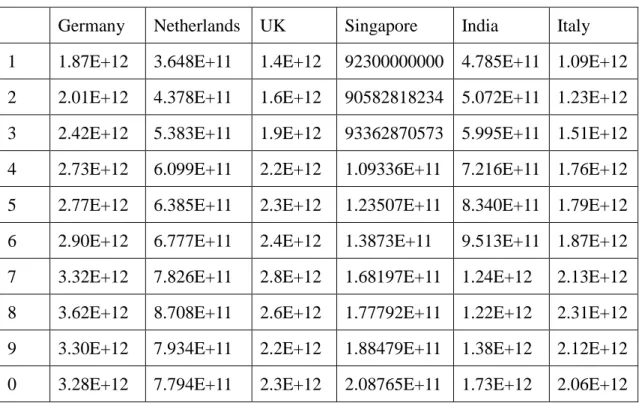
Table A4 (1): GDP of China and ten main economies (dollars)
dollar China United States Hong Kong Japan Korea, Rep. 2001 1.0799E+12 9.8374E+12 1.626E+11 4.8416E+12 4.572E+11 2002 1.45383E+12 1.05902E+13 1.63781E+11 3.91834E+12 5.75929E+11 2003 1.64096E+12 1.10892E+13 1.58572E+11 4.2291E+12 6.43762E+11 2004 1.93164E+12 1.18123E+13 1.65886E+11 4.60592E+12 7.21975E+11 2005 2.2569E+12 1.25797E+13 1.77772E+11 4.5522E+12 8.44863E+11 2006 2.71295E+12 1.33362E+13 1.89932E+11 4.36259E+12 9.51773E+11 2007 3.49406E+12 1.3995E+13 2.07087E+11 4.37794E+12 1.04924E+12