J
Ö N K Ö P I N GI
N T E R N A T I O N A LB
U S I N E S SS
C H O O L Jönköping UniversityStock Market Anomalies
A Literature Review and Estimation
of Calendar affects on the S&P 500 index
Bachelor thesis in economics
Author:
Marcus Davidsson
Head Supervisor:
Per-Olof Bjuggren
Deputy Supervisor 1: Daniel Wiberg
Deputy Supervisor 2: Helena Bohman
Jönköping, 2006-02-05
Bachelor Thesis in Economics Title: Stock market anomalies Author: Marcus Davidsson
Tutor: Per-Olof Bjuggren, Daniel Wiberg & Helena Bohman Date: 2006-02-05
Subject terms: Anomalies, S&P 500, Calendar affects
Abstract
This thesis investigates the Day-of-the-week, Month-of-the-year and Quarter-of-the-year effects. Historical data from the S&P 500 index between 1970- 2005 is analyzed. The purpose is to investigate if there is any evidence of increased returns (ROR) pattern related to seasonality during this period. The conclusion is that Wednesdays, December and Quarter 4 had the highest ROR while Mondays, September and Quarter 3 had the lowest ROR.
The empirical analysis found support for the Monday effect that Mondays are the days with the lowest stock returns. An investor would have earned on approximately four times more if you invested on Wednesdays instead of Mondays. Mondays was the only days with a negative ROR. I also found support for the weekend effect that return on Fridays are higher than returns on Mondays. However this weekend effects may have been given too much attention and appear to be somewhat overrated. Based on the empirical analysis a mid-of-the-week effect or Wednesday effect is more noticeable than the weekend effect. This is some what different from previous studies.
No support was found for the January effect that stock prices should be higher in January than in December. What I however clearly could see was a September effect. September is the only month with negative returns. You would have on earned approximately three times as much if you invest in the beginning of December instead of the beginning of September. This leads to that the quarter 3 should be avoided due to a negative historical aggregated ROR. Quarter 4 on the other had the highest return. If you would have invested in quarter 4 instead of quarter 3 you would historically have earned approximately four times as much.
Table of contents
1-Introduction ...
4
2-Literature Review...
5
2.1 Efficient market theory and fundamental value 'anomalies' ...
5
2.2 Calendar anomalies ...
7
2.3 Other anomalies ...
8
3-Data and basic definitions ...
11
3.1 Data the S&P-500 index ...
11
3.2 Overview of price development, volumes and yearly ROR...
11
3.3 Limitations and basic definitions ...
14
4-Empirical analysis ...
15
4.1 Day-of-the-week effect ...15
4.2 Month-of-the-year effect ...16
4.3 Quarter-of-the-year effect ...17
5-Conclusions ...
18
References...
19
Appendix...
24
Figures, Tables and Appendix
Figure 3.1 Price development of the S&P-500 Index from 1970-2005 Figure 3.2 Percentage ROR of the S&P-500 Index from 1970-2005 Figure 3.3 Arithmetic averages of daily traded volumes 1970-2005 Figure 3.4 Accumulated yearly ROR units 1970-2005
Figure 4.5 Average daily ROR 1970-2005 Figure 4.6 Average monthly ROR 1970-2005 Figure 4.7 Average quarterly ROR 1970-2005 Table 2.1 Calendar anomalies
Table 2.2 Other stock market anomalies
Table 4.3 Regression results day dummy variables Table 4.4 Regression results month dummy variables Table 4.5 Regression results quarter dummy variables Appendix-1 Basic definitions
Appendix-2 Overview ROR calculations
Appendix-3 Regression between ROR and day-dummies Appendix-4 Regression between ROR and month-dummies Appendix-5 Regression between ROR and quarter-dummies
1-Introduction
The quantity of studies finding evidence of different market anomalies are too overwhelming to simply ignore and just write off as temporary miss-pricings according to efficient market theory. Analysing market data and anomalies give important indications of how well current theoretical frameworks describe reality by clarifying their limitations. This has important implementation when it comes pushing our understanding further by laying the groundwork for future theories. However careful analysis has to be done for each individual phenomenon not to exaggerate the importance and significance of single observation. Investors have to be critical not to over-interpret results with the risk of neglecting and underestimating the importance of such a basic concept as portfolio diversification
The basic question related to market anomalies is whether an identified anomaly is evidence of a stable and long run phenomenon which an investment strategy could be based on or if it is just as the names suggest a short-term unique miss pricing. EMT is flexible in this sense; the theory acknowledge that there might exist short term anomalies but that these will in a longer perspective be cancelled out so that the market can go back to being perfectly efficient. There is no guarantee that markets will be perfectly efficient in the short run however an investor specialised in detecting anomalies and arbitrage opportunities will not be able to attract any abnormal returns due to the sporadic nature of these anomalies. Short term miss-pricing do exit and according to efficient market theory, impossible to identify.
Cross (1973) examined the S&P 500 index but with a different time period between the periods 1953 to 1970 and found that, on average, returns on Fridays are higher than returns on Mondays. I want to investigate if this is still true thirty-two years later? Other studies that have been based on different data sets are for example Gao & Kling (2005) that investigates calendar effect in Chinese stock market. They used Shanghai and Shenzhen index between the periods 1990 to 2002. They found that the month with the highest return is March and April and that Fridays have in general higher returns than other days. They explain that the Chinese year ends in February. Their findings that March and April had higher returns are therefore inline with other studies based on the western calendar year. This leads to the question is this month-of-the-year effect present in other data sets?
There are three things that hopefully will distinguish this thesis from many others. The first differentiating factor is the some what ambiguous presentation and review of the large quantity of stock market anomalies that are available in empirical studies and articles. The second thing that hopefully will distinguish it even further is the clear and straightforward review of the surrounding framework regarding for example concepts and methods. The third thing is a more diversified focus on three major stock market anomalies instead on a single anomaly. This is a result of economics of scales related to the data mining. Market timing is essential and highly critical for an investor. Hopefully this paper will lead to a somewhat increased understanding of the relationship between market timing and ROR. The purpose of this thesis is to investigate the day-of-the-week, month-of-the-year and quarter-of-the-year effects in historical data from 1970- 2005 on the S&P 500 index. The problem questions that this thesis will answer are the following:
- Is there any evidence of the day-of-the-week effect? - Is there any evidence of the month-of-the-year effect? - Is there any evidence of the quarter-of-the-year effect?
2-Literature Review
2.1 Efficient market theory and fundamental value “anomalies”
The efficient market theory (EMT) evolved from Eugene Fama’s dissertation “The Behaviour of Stock Market Prices” in 1965. Later in 1965 it was summarized and republished as
"Random Walks in Stock Market Prices”. The most important notion of the theory is that an
investor can only get increased returns by taking on more risk (keeping interest rates fixed; increased interest would result in a higher expected ROR). Farma (2004) explain that it is the risk that you can not diversify away that you get compensated for. Efficient market theory states that “prices reflect all available information. In a perfectly efficient market it is impossible to beat the market. Investors are always paying a “fair price”. This means that the only thing investors have to worry about is choosing which risk-returns-trade-of they want to be involved with.” Since the 1960’s there have immerged numerous studies questioning the degree of market efficiency and the static assumptions behind for example EMT & CAPM1, 2 Fields like behavioural-economics and -finance have received much deserved attention for their more flexible & detailed view regarding neoclassical economic agents and markets. Fama (2004) explains that people like Warren Buffett, who have evidently been successful in the stock market, have chosen a few stocks over a long period of time. Farma explains that it is impossible for an investor like Warren to successfully pick a large selection of stocks during a shorter time period and still earn abnormal returns due to market efficiency. Since the original paper was published in the 1960 Fama has developed his reasoning further and have become a little bit more “anomaly friendly” if you so like, compared to a somewhat holistic & reserved original view. In the paper by Fama & French (1992) which turned the investment community on its head, they extend the CAPM, which is based on the assumption of economic efficiency, to construct what they call a three factor model.
The CAPM model has suffered from obvious limitations concerning the way it calculates market returns but also in the way it quantify market risk, beta. Fama & French (1992) realized that the classical CAPM formula may not be suitable for all type of firms. They therefore added two other variables to the already existing framework, a size variable and a value variable in form of a book-to-market ratio. They found that the two new introduced variables where highly correlated with market returns. The cost of capital for smaller or high book-to market firms is significantly higher than predicted by the CAPM. The implication of this is that it exist other types of risks than just overall market risk inform of beta. Fama & French (1992) classifies them as size risk and distress risk which is related to value variable: book-to-market ratio or other similar measures such as cash flow to price and earnings to price. Critics argued that these extra variables are evidence of that anomalies do exists and that markets are not effective. Fama & French (1992) explains that this is not the case. Size and book-to-market ratio are not anomalies according to them; they are related to the risk that investors get compensated for.
There exists many different fundamental value “anomalies” Reiganum (1981), Banz (1981) & Fama & French (1992, 1993) explains that the Size or Market equity (P*Q) effect is the notion that small firm’s on average have higher returns than large firms. This is related to according to French (2004) that “small stocks usually have higher volatilities than larger once and therefore intuitly requires higher rates of returns”. Sharpe, Capaul, & Rowley (1993) &
1 The model is based on the work by Sharpe, Lintner & Mossin in the 1960’s.
Fama & French (1992, 1993) explains the Book-to-market (BE/ME)3 effect, Price-to-book (P/B) effect or the Value effect as it is also called is related to the notion that distress stocks or “value stocks” stocks with a low valuation and low price-to-book ratio (high BE/ME), earn on average higher returns than growth stocks, stocks with a high valuation and high price-to-book ratios. Fama & French (1992) analysed data from the period 1963-1990 from a cross-section of countries and found that the premium for investing in value stocks instead of growth stocks was about “three and half to four percent”. Value stocks are more risky and therefore require a higher rate of return. Other studies have found somewhat different results. Lee & Song (2002) found for example that “value stocks tend to outperform growth stocks around recession periods”.
Fama & French (1992, 1993) explain that value stocks dose not tend to have higher volatility than growth stocks. This leads to that measuring risk based only on volatility seems to have its limitations. However an investor should never forget that investing in small, undervalued firms always results in extra risk i.e. extra bankrupts risk. An extra point to add here is that a stock that have depreciated heavily (high volatility) is not seen by growth investors as a risky stock but rather as a cheap stock and vise versa. French (2004) “explain that it gives an investor a framework for portfolio allocation decisions, am I comfortable with the overall exposure to the stock market, am I making the right trade-off between the extra expected return from small stocks and the extra risk that it brings and am I making the right trade-off between the extra expected return I get from buying distress stocks and the extra risk that it brings”. There dose also exist other factors that has to be taken in to consideration i.e. tax issues. French (2004) also explains that it dose not exist an “optimal portfolio” in the end it all comes down to personal preferences about risk and return.
The list of potential causal variables doesn’t end here. There are numerous other anomalies which will briefly be discussed below (Guin, 2005). Basu (1977) observed something called the Price-to-earnings (P/E) effect which means that stocks with low P/E ratios have a propensity to outperform stocks with high P/E ratios with on average about seven percent per year. French, (1992) explain that an investor can outperform the market with for example low P x Q, P/B or P/E stocks but only because he is taking on more risk. Another anomaly is called the Price-to-sales (P/S) effect. Guin (2005) explain that stocks with low price to sales ratios tend to outperform the market and stocks with high price to sales ratios. Chan, Hamao & Lakonishok (1991) discusses the so called Price-to-cash flow (P/CF) effect which states that stocks with low price to cash flow ratios tend to produce higher returns than predicted by the CAPM. The critique of efficient market theory is that it is easy to just claim that high risk stocks will on average result in high return. It is like saying: if you stand in the middle of the road and a high speed lorry approaches then the chance of being killed is greater than the chance of being killed by a man on a high speed bicycle. The reasoning is somewhat undynamic because it leaves the most important question unanswered. Is the compensation for an investor that invests in high risk stocks sufficient?
If you invest in small stocks or stocks with high P/E ratios then you take the increased chance of gaining a lot but also the risk of losing a lot. Therefore the question of how much an investor get compensated for the extra risk associated with investing in for example value stocks instead of growth stocks becomes the most crucial question an investor can ask. This leads to that arbitrage and anomalies become more interesting. If an investor has knowledge
3 Book-to-market is defined as “book equity/ market equity, where book equity is book value of shareholders equity+ deferred taxes and tax credits- book value of preferred stock and market equity is the size effect price* shares outstanding. (French, 2004)
about arbitrage opportunities and market anomalies then he has at least some chances of getting compensated for the risk he is taken on. This of course assumes that markets are not perfectly efficient which the majority of studies are supporting. Investor (2004) points out an important fact that “markets are neither perfectly efficient nor completely inefficient. All markets are efficient to a certain extent, some more so than others. Rather than being an issue of black or white, market efficiency is more a matter of shades of grey”
Another important fact is the paradox of efficient market theory, “if every investor believed that markets were efficient then the markets would not be efficient because no one would analyze securities! In effect, efficient markets depend on market participants who believe the market is inefficient and trade securities in an attempt to outperform the market” (Investor, 2004). “This reasoning provided by Farma & French is exactly the opposite of what a traditional business analyst would tell you. The difference comes from whether you truly believe in the efficient market theory or not. The traditional business analyst doesn’t agree with the notion of market being perfectly efficient. He thinks he has a greater probability of picking winning stocks than the average market. “This traditional business analyst would say that a firm with high book/price indicates a buying opportunity: the stock looks cheap. But if you do believe in EMT then you believe cheap stocks can only be cheap for a good reason, namely that investor’s think they're risky” (Chimp, 2004).
2.2 Calendar anomalies
Calendar or time anomalies seem to exist everywhere. The following table will describe a sample of calendar anomalies that are relevant for this thesis.
Table 2.1 Calendar anomalies
Effects Authors Findings
Month-of-the-year effect or January effect
Keim (1983), Ariel (1987) & Haugen and Jorion (1996)
Stock prices are usually higher in the first two weeks in January than in the end of December. Turn-of-the-year
effect
Dyl (1977) & Givoly and Ovadia (1983)
Trading volume is usually larger for example losing stocks in December.
Guin (2005) This has to do with tax-related issues, selling in December and buying in January.
Summer effect Wachtel (1942) He found evidence of a rising stock prices in the summer
Month-of-the-quarter effect
Penman (1987) Firm’s usually have higher rate of returns in the first month of the quarter.
Week-of-the-month effect
Linn & Lockwood (1988) and Hensel and Ziemba (1996)
Stocks usually have higher returns during the first week of the month than the last thee. Day-of-the-week
effect or Weekend effect
Cross (1973) and French (1980)
On average, closing price on Monday evening are lower than Fridays closing prices a
Guin (2005) “The weekend effect can be related to that companies and governments tend to realize bad news over the weekends”
Foster and
Wiswanathan (1990)
Trading volumes are increasing on Fridays due to information symmetry and decreasing on
Mondays due to information asymmetry. Monday effect French (1980), Barone
(1990) and Gibbons & Hess (1981)
Average returns on Mondays are lower than any other day of the week. They also found that the largest decrease in stock prices takes place during the first two days of the week.
Hour-of-the-day effect or the End-of-the-day effect
Guin (2005) Trading volumes and prices tend to increases during the last 15 minutes of a day.
Harvey and Huang (1991)
Noticed higher interest rates volatility during Thursdays and Fridays first trading hours. Holiday effect Lakonishok & Smidt
(1988) and Petengill (1989)
Stock markets usually tend to have higher abnormal returns before public holidays.
Political-cycle effect,
Santa & Valkanov (2003)
The first and last year of a presidential administration period have higher abnormal returns than the other years.
2.3 Other Stock market anomalies
There also exist other anomalies that cannot be classified as either called calendar anomalies or fundamental value anomalies which will be described in the table below: Farma (2004) explain that the problem with anomalies in general is that “after anomalies are documented and analyzed in the academic literature, anomalies often seem to disappear, reverse, or attenuate” due to market equalisation
Table 2.2 Other stock market anomalies Stock-split effect Fama, Desai &
Jain (1997) and Ikenberry et al. (1996)
A stock split tends to increases the share price of a company both before and after the stock splits is announced. Dividend-per-price effect or Dividend- yield effect Litzenberger & Ramaswamy (1982) & Levis (1989)
Stocks with high dividend yields tend to outperform the market on average
Keim (1985) Smaller firms have usually higher dividend yields than larger once
Low-prices-stocks effect
Guin (2005) “Stocks that have a low price tend to do better than high price stocks. The basic assumption is that earnings drop while sale remains constant. A drop in earnings is not as bad as a drop in sales. If the sales hold up, the management can eventually solve the earnings problem causing the stock price to rise. If both sales and the price drop an investor should avoid that stock”. Neglected-firm
effect,
Arbel & Strebel (1983) and Guin
Firms that have been neglected by institutional investors usually generate higher returns than
(2005) those covered. The ideal situation occur when stocks begins to be covered by analysts Momentum effect Jegadeesh and
Titman (1993).
“Stocks that have out performed the market usually continue to do so for an intermediate period of time, three to five years on average”. Due to this momentum you should sell value stocks and buy growth stock. (Guin, 2005) Lee & Song
(2002) in Asness (2000)
Value strategies are strongest among low-momentum stocks, and the low-momentum strategy is strong among growth stocks”.
Farma (2004) (Schwert, 2003)
The problem with an “tradable momentum investment strategy is that you have to turning the portfolio over as time goes by which might lead to that the cost overweight the benefits”. Reversion to the mean long-term effect (negative autocorrelation) DeBondt and Thaler (1985). Guin (2005)
Stock prises tend to reverse over long cycles of time which means that the biggest loser over the past three to five years tend to be the biggest gainers over the next three to five years on average
Earnings surprise effect,
Guin (2005) “Stocks which report earnings considerably different from the consensus earnings forecasts tend to move by exceptional amounts. This price movement continues for up to several weeks after the announcement, meaning that an investor can still profit from the information, even though it has been made public.”
Reversion to the mean effect short-term effect
DeBondt and Thaler (1985). Guin (2005)
“Stocks that has outperformed one month tend to under perform the next month (and vice versa). However, this is true only if the performance is not caused by an earnings surprise. If the change in price is due to an earnings surprise, it is more likely that the performance will persist. Stocks which have experienced a recent reduction in their P/E ratios tend to have higher rates of return than other stocks”. (Guin, 2005)
Late earnings reporter effect
Guin (2005) “Firms that report their earnings later than others in the industry often have poor results to announce. Therefore, companies which have not announced earnings by their usual date should be avoided” Insider transaction effect Finnerty (1976) & Lakonishok and Lee (2001)
Insiders are well informed and earned above average returns and can in some cases even predict changes in stock prices.
Information releasing effect,
Wilandh & Johansson (2005)
Information release events create an “adverse selection problem, where the uninformed investors have a disadvantage in terms of information.” The authors showed a significant decrease in trading volume before a scheduled announcement. After the announcement and the
“corporate information is released the
information asymmetry is resolved, which leads to an increase in trading volume”.
Market overreaction effect
Shiller (1981) Stock market tends to overreact to news about future dividends.
Yulong, Tang & Tanweer (2005)
Found evidence of the overreaction and reversal effects on the Nasdaq stocks market. The authors also explain that “stock price usually reverses itself after the stock experiences a sharp increase or decrease in price”.
Market under reactions effect
Abarbanell and Bernard (1992)
Both analysts and the market tend to under react to earnings announcements
Post-Earnings announcement drift effect
Ball & Brand (1968) in Fama (1997)
“Stock prices seem to respond to earnings for about a year after they are announced”
Country specific effect
Gultekin & Gultekin (1983)
For example the degree of the month-of-the-year effect in different countries varies; the effect in USA is smaller.
IPO effect 1 Jong-Hwan
(2003)
“There exist evidence of an under pricing phenomenon of IPO’s which results in positive average abnormal return found over a short period of time after the issue”.
IPO effect 2 Ritter (1991) In the long run, after 3 years of going public, these firms significantly under performed market performance”.
IPO effect 3 Raghuram & Servaes (1996) and McNichols and O'Brien (1996)
“Analysts are overoptimistic about the earnings and growth performance of IPO’s” (Raghuram & Servaes, 1996) This over optimism may be a result of selection bias; “analysts typically start following stock they are optimistic about” (McNichols and O'Brien, 1996)
Index effect Harris & Gurel (1986)
“Stocks prices seams to rise immediately after a companies stock has been added to for example the S&P 500 Index. An investor should buy the stocks that will be added to the S&P 500 index, after the announcement but before the stock is added”. (Investor, 2004)
As the reader can see and verify, there exist a ton of stock market anomalies. The list is far from complete and perfectly representable. The most famous of them all Bubbles are not dealt with in order to limit the scope of this thesis. A continuous presentation of numerous other anomalies will not benefit this thesis. I will therefore not describe any more stock market anomaly in order to allocate more attention to the empirical study of the day-of-the-week effect, month-of-the-year effect and the quarter-of-the-year effect that have been chosen for the empirical section of this thesis. I hope that this systematic presentation has helped the reader to form an overview and introduction to different stock market anomalies.
3-Data and basic definitions
3.1 Data the S&P-500 index
The historical data from 1970-2005 on the Standard & Poor 500 index was extracted from the webpage of Yahoo finance. The data consisted of daily and monthly closing prices, volumes and dates.. Motley (2005) explains that S&P 500 index is a market capitalization weighted index. This means that each companys market value is proportional to the index weight. “The companies that makes up the index represent 500 of the most widely held U.S.-based common stocks, chosen by the S&P Index Committee for market size, liquidity, and sector representation, leading companies in leading industries" is the guiding principal for S&P 500 inclusion”. “A small number of international companies that are widely traded in the U.S. are included, but the Index Committee has announced that only U.S.-based companies will be added in the future” (Motley, 2005).
Larger companies account for a greater share of the index. This is different from a price weighted index such as the Dow Jones Industrial Average that gives higher priced stocks more weight than lower priced stocks. “The S&P 500 represents approximately 70% of the value of the U.S. equity market. The 500 listed companies represent a diverse range of industries, spanning every relevant portion of the U.S. economy.
The S&P 500 index is comprised primarily of U.S.-based companies”. The S&P 500 index is an important indicator of overall US market performance. This is especially true for large cap stocks. The index work as an important benchmark of active portfolio fund managers to evaluate their performance compared to the overall stock market.
Motley (2005) also explains that the S&P 500 have “significant liquidity requirements for its components, so some large, thinly traded companies are ineligible for inclusion. Because the index gives more weight to larger companies, it tends to reflect the price movement of a fairly small number of stocks”. This is also one of the index drawbacks. (Motley, 2005)
Investors that want to follow the index dose not have to buy all 500 companies which would be quite hard. Instead they can buy exchange traded funds (ETF) called Spiders which tracks the S&P 500 index.
3.2 Overview of price development, volumes and yearly ROR
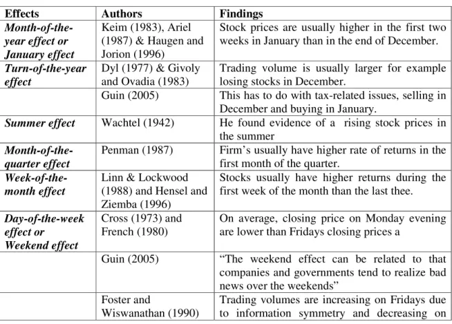
In figure 3.1 we can see that the price of the S&P-500 Index have steadily increased since 1970. What is striking is the steady development and accumulation of wealth the index the index has provided. This reinforces the appropriateness of a basic investment strategy such as 50/50 meaning 50 percent in equity index funds and 50 percent in fixed income. Leverage with stocks market index funds is a more vice long term investment instead of taking the excessive risk of trying to pick individual winning stocks. This figure also indirectly shows that there are probably very few active portfolio managers that can on a regular basis beat a yearly average rate of return of nine percent. Stock index funds are however not without risk. We can see that there has been a tough period around the millennium shift the years 2000, 2001 and 2002 where we had approximately three years of bear market with a depreciation of about thirty percent.
Figure 3.1 Price development of the S&P-500 Index from 1970-2005
In figure 3.2 we can see the volatility of S&P-500 index returns. We can see more clearly that stock index funds are not without risk. I have divided the ROR into four different categories: extreme low, extreme high, low and growth. The two first categories are not that relevant since the first category more or less compensate for the second one. The years 2002, 2001, 2000, 1994, 1990, 1981, 1977, 1974, 1973 and 1970 had all negative returns between 1 and -29 %. 28 % of the total years had negative returns. These extreme low years are compensated by only four extreme good years 1997, 1995, 1989 and 1975 which had returns between 34 and 27%. These extremely good years represent 11% of the total years. The total ROR for these categories is zero (124% and -124%)
The third category of low growth consists of five years 2005, 1992, 1987, 1984, 1978 with ROR between 1 and 5 % and accounts of approximately 14%. This ROR are considered low since they all are position below or slightly above the average yearly inflation rate of 3, 4% which is not sufficient. The most interesting period is the fourth category, growth. The years classified in this period have ROR between 7 and 26 %. This period represent approximately 50% of the total years but accounts for 96% of the total ROR. The yearly average rate of return during the total 35 years is approximately nine percent.
-30 -25 -20 -15 -10 -5 0 5 10 15 20 25 30 2 0 0 5 2 0 0 4 2 0 0 3 2 0 0 2 2 0 0 1 2 0 0 0 1 9 9 9 1 9 9 8 1 9 9 7 1 9 9 6 1 9 9 5 1 9 9 4 1 9 9 3 1 9 9 2 1 9 9 1 1 9 9 0 1 9 8 9 1 9 8 8 1 9 8 7 1 9 8 6 1 9 8 5 1 9 8 4 1 9 8 3 1 9 8 2 1 9 8 1 1 9 8 0 1 9 7 9 1 9 7 8 1 9 7 7 1 9 7 6 1 9 7 5 1 9 7 4 1 9 7 3 1 9 7 2 1 9 7 1 1 9 7 0
Aithmetric Mean
Geometric Mean
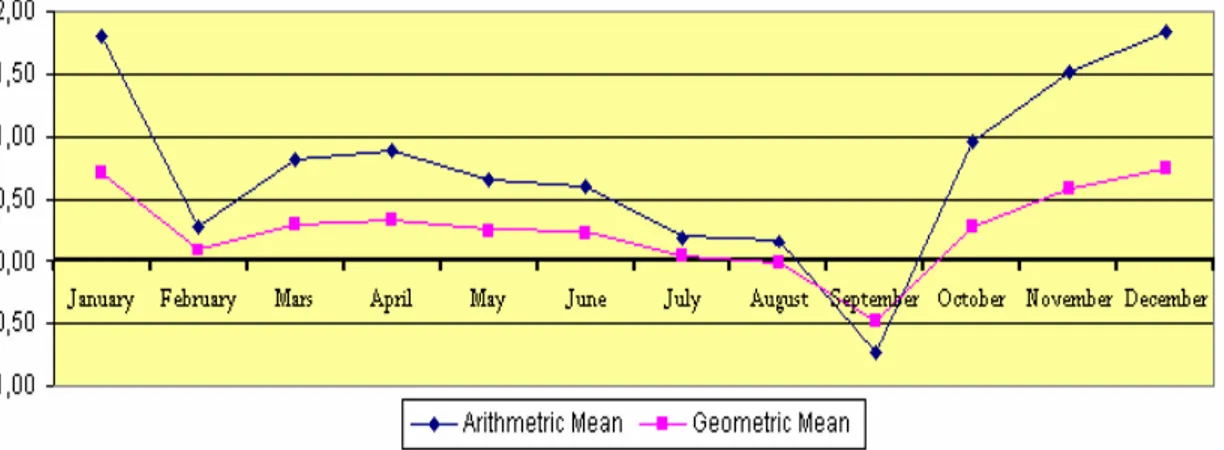
In the third figure 3.3 the increase in traded volumes that has occurred during this period is presented. From 1970 to 1984 the volumes were very low. Since 1984 the traded volumes have exploded. By looking at the figure below we can see that the volumes have ruffle increased by eighteen times since 1990. This is a huge increase for a time period of only fifteen years. We can also see a time lag after the recession in 2000. It took up till 2002 until the momentum of increased volumes flattened out. We can also see that the volumes were kept at the same level for a year and then people seemed to forget about the recession and starting buying again with a result of increased volumes.
Figure 3.3 Arithmetic averages of daily traded volumes 1970-2005
In figure 3.4 we can once again the large accumulation of wealth the S&P-500 index has provided. The accumulated yearly rate of return units from 1970 to 2004 was approximately 315 percent. This means that the yearly percentage unit change has been around nine percent. As we saw before there were three tuff years in 2000, 2001 and 2002. However we can see below in figure 1.6 that this decline has only a small effect on the total accumulated ROR. We can see that there were some tuff years in the beginning and in 1974, 1975 and 1981
3.3 Limitations and basic definitions
There exist two main limitations with statistics. The first limitation is, as we learned from a basic statistics course, that correlation is not the same as causation. Variables can be highly correlated without a cause-effect relationship. Statistics is about determining correlation. Causation on the other hand is based on theory and tested by for example controlled experiments. The second problem is related to the scope of variables. In real life outcomes (at least the interesting ones) are affected by many complex and dynamic layers of variables. If some variables, for any reason, are excluded from the analysis (this is nearly always the case in social science) then there will not exist a high degree of correlation between historical data and future statistical predictions. Because of these two reasons it is important to always maintain a critical perspective when it comes to using statistics in for example investment decisions. Usually historical data is a good approximation of historical risk but a poorer approximation of future returns. Below is a review some basic definitions in order for the reader to get a better understanding of the conceptual framework.
Discrete or arithmetic ROR is based on the notion that the FV=PV*(1+g) where g= percentage growth. Discrete ROR are always larger than continuous ROR. FV of the price (P) at time t can be expressed as: Pt= Pt-1*(1+ROR) gives 1+R= Pt/ Pt-1 which gives the proportional change R= (Pt/ Pt-1)-1. ROR can also be expressed as % change R= (Yt-Yt-1) / Yt-1 which is equal to the proportional change Yt / Yt-1 – Yt-1 / Yt-1= (Yt /Yt-1) -1. ROR could also be expressed as absolute change ROR= Pt -Pt-1 however then we could not make comparisons between series with different price units. The arithmetic mean can be expressed as AM ROR= (R1+ R2...Rn)/ n where R=discrete percentage returns and n= number of ROR. Below on the left-hand side is the expression for the yearly arithmetic return. Were VT and VO are the prices of the asset at the first and last trading day of the year and Vt is the price at time t. Asa (2004) states “yearly arithmetic returns cannot be expressed as the sum of the daily arithmetic returns”.
Continuous compounded (CC) ROR, Geometric or Log returns can be expressed as the FV= PV*e^ g4 where g=growth and e=Euler constant 2, 718... The natural logarithm ln follows the same laws as the common logarithm. [ln(1)=0 ln(e)= 1, ln(e^ x)=x and e^ ln(a)= ln(e^ a)= a ].PV=FV/ e^ g or PV=FV*e^-g or PV=FV*1/ (e^ g). The FV of the price (P) at time t can be expressed as Pt= Pt-1*e^ ROR Hence e^ ROR= Pt/ Pt-1 and the rate of return or the percentage change can be expressed as: ROR= ln (e^ ROR) = ln (Pt/ Pt-1)*100=ln (1+Rt)*100. ln (Pt/ Pt-1) can also be written approximately as5: ln(Pt)- ln(Pt-1. For a deeper discussion of basic definitions and concepts see appendix 1.
4 FV=PV*e^ g can also be expressed as: ln(FV)= ln(PV)+ln(e^ g) where ln(e^ g)=g due to the logarithm rule: ln(x*y) =ln(x) + ln(y) e^ g can also be written as exp^ g
4-Empirical analysis
4.1 Day-of-the-week effect
Zero transaction costs are assumed and that the investor is a day, month and quarter trader. The following econometric model was tested: Y =B D1 1+B D2 2+...B D5 5+εt where D1, D2,
D3… is the dummy variables for each day. This econometric model resulted in the equation presented below. The slope parameters can also be seen in figure 4.5 below. T-statistics are presented in table 4.3. We can clearly see that D3 Wednesday was the only day that was significant with a t-statistic of 3, 35. The R^2 adj value is not that interesting since we don’t have any independent variables. See appendix 3 for more details.
ROR= -0.026*D1+0.045*D2+0.077*D3+0.022*D4+0.045*D5
Table 4.3 Regression results day dummy variables t-statistics
D1 D2 D3 D4 D5
-1,1052767 1,9596853 3,351243 0,9800689 1,9229493
This can also be seen in figure 4.5 below. Here we see that Wednesday had the highest daily return of 0, 08 percent. This may not seem so much but remember that we are taking about daily returns and not annual. The daily rate of return is the return an investor gets if he only trade during a specific weekday, meaning that he buy at the opening price and sell at the closing price, for example, every Monday of the year. The aggregated daily rate of return units on Wednesday is equal to 143.12 percentage points. This can be compared to -45.55 on Monday, 83.64 on Tuesday, 41.42 on Thursday and 81.02 on Friday. The mean for all weekdays was 60.73. See appendix 2 for more details.
Figure 4.5 Average daily ROR 1970-2005
The average GM for all days is equal to 0.011. Wednesdays is the weekday with the highest ROR. If you only invested on Wednesdays you would have got a return of 3 times the average ROR of all weekdays. The day you should avoid is Monday with a negative aggregated ROR of -45.55%. An investor would have earned approximately four times more if you invested on Wednesdays instead of Mondays. If you rank the weekdays according to highest ROR the series becomes: Wednesday, Tuesday, Friday, Thursday and Monday.
4.3 Month-of-the-year effect
The following econometric model was tested: Y =B M1 1+B M2 2+...B M12 12+εt
Where M1, M2, M3… is the dummy variables for each month. This econometric model resulted in the equation presented below. The slope parameters can also be seen in figure 4.6 below The t-statistics are presented in table 4.4. We can clearly see that M1 January, M11 November and M12 December was the only months that were significant with a t-statistic of 2.41, 2.03 and 2.47 respectively. See appendix 4 for more details.
ROR= 1.80*M1+0.28*M2+0.81*M3+0.90*M4+0.65*M5+0.61*M6+0.20*M7+0.17*M8 -0.97*M9+0.96*M10+1.51*M11+1.84*M12
Table 4.4 Regression results month dummy variables t-statistics
M1 M2 M3 M4 M5 M6
2,418196223 0,391117092 1,105724685 1,22241775 0,89180109 0,8332697
M7 M8 M9 M10 M11 M12
0,275738271 0,229894292 -1,324617336 1,29543578 2,032181 2,471162
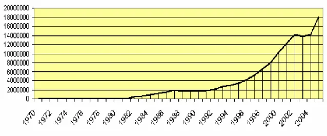
This can also be seen in figure 4.6 below. Here we see that December followed by January and November had the highest monthly return with 1.84, 1.80 and 1.51% respectively. Again this may not seem so much but remember that we are taking about monthly returns and not annual. The monthly rate of return is the return an investor gets if he only trade during a specific month, meaning that he buy at the opening price and sell at the closing price, for example, every January of the year. The aggregated daily rate of return unit for December followed by January and November is 64.66, 63.27 and 53.17 percentage points respectively. This can be compared to 10.38 in February, 29.34 in Mars, 32.44 in April, 23.66 in May, 22.11 in June, 7.32 in July, 6.10 in August, -35.15 in September and last but not least 33.89 in October The mean for all months was 25.93. See appendix 2 for more details.
Figure 4.6 Average monthly ROR 1970-2005
The average GM for all months is equal to 0.253. December followed by January and November had the highest monthly ROR. If you only invest in December, January or November you would have got a return of 3, 2.7 and 2.3 times the average GM ROR of all months. The month you especially should avoid is September with a negative aggregated ROR of -35.15%. This leads to that you would have earn approximately three times as much
if you invest in the beginning of December instead of the beginning of September. If you rank the months according to highest ROR the series becomes: December, January, November, October, April, Mars; May, June, February, July, August and September.
4.4 Quarter-of-the-year effect
The following econometric model was tested: Y =B Q1 1+B Q2 2+...B Q4 4+εt
Where D1, D2, D3… is the dummy variables for each quarter. This econometric model resulted in the equation presented below. The slope parameters can also be seen in figure 4.7 below The t-statistics are presented in table 4.5. We can clearly see that Q4 is the only quarter that was significant with a t-statistic of 3.11. See appendix 5 for more details.
ROR= 2.68*Q1+2.26*Q2-0.51*Q3+4.33*Q4
Table 4.5 Regression results quarter dummy variables t-statistics
Q1 Q2 Q3 Q4
1,954010629 1,65012842 -0,377534729 3,1173106
This can also be seen in figure 4.7 below. Here we see that quarter 4 had the highest quarterly return of 4.33 percent. Once again this may not seem so much but remember that we are taking about quarterly returns and not annual. The quarterly rate of return is the return an investor gets if he only trade during a specific quarter, meaning that he buy at the opening price and sell at the closing price, for example, every quarter 1 of the year. The aggregated quarterly rate of return unit in quarter 4 is equal to 151.87 percentage points. This can be compared to 96.54 in quarter 1, 81.53 in quarter 2 and -18.65 in quarter 3. The mean for all quarters was 77.82. Quarter 4 is the quarter with the highest ROR. If you only invested in quarter 4 you would have got a return of 2 times the average ROR of all quarters, 77.82. The quarter you should avoid is quarter 3 with a negative aggregated ROR of -18.65. An investor would have earned approximately four times more if he invested in quarter 4 instead of quarter 3. If you rank the quarters according to highest ROR the series becomes: quarter 4, quarter 1, quarter 2 and quarter 3. See appendix 2 for more details.
5-Conclusions
The result from the empirical analysis are summarized and presented below. The conclusions are ordered according to the problem questions in order to maintain a clear structure.
- Is there any evidence of the day-of-the-week effect?
Yes there is evidence of a day-of-the-week effect. Wednesdays is the weekday with the highest ROR. The empirical analysis also found support for the Monday effect that Mondays are the days with the lowest stock returns. Mondays was the only day with a negative return. The empirical analysis also found support of the weekend effect that returns on Friday is higher than returns on Mondays however this weekend effects may have been given too much attention. Based on the empirical analysis a mid-of-the-week effect or Wednesday effect is more noticeable than the weekend effect. If you only invested on Wednesdays you would have got a return of 3 times the average GM ROR of all weekdays. An investor would have earned approximately four times more if you invested on Wednesdays instead of Mondays
- Is there any evidence of the month-of-the-year effect?
Yes there is evidence of a month-of-the-week effect. December followed by January and November had the highest monthly ROR. However based on the empirical analysis I do not find any support for the January effect that stock prices should be higher in January than in December. Another thing that I clearly can see is a September effect. September is the only month with negative returns. Buying stocks in the beginning of September should therefore historically been avoided. If you only invest in December, January or November you would have got a return of 3, 2.7 and 2.3 times the average GM ROR of all months. This leads to that you would have earn approximately three times as much if you invest in the beginning of December instead of the beginning of September.
- Is there any evidence of the quarter-of-the-year effect?
Quarter 4 is the quarter with the highest ROR. If you only invested in quarter 4 you would have got a return of 2 times the average ROR of all quarters, 77.82%. The quarter you should avoid is quarter 3 with a negative aggregated return. An investor would have earned approximately four times more if you invested in quarter 4 instead of quarter 1. If you rank the quarters according to highest ROR the series becomes: quarter 4, quarter 1, quarter 2 and quarter 3.
References
Abarbanell, J and Bernard, V (1992) Test of Analysts' overreaction/ under reaction to Earnings Information, Journal of Finance 47 (1992): 1181-1207.
Asness, C (2000) The interaction of value and momentum strategies,
Financial Analysts Journal 56, 29-36.
Arbel, A & Strebel, P (1983) Pay Attention to Neglected Firms,
Journal of Portfolio Management, 37-42.
Ariel, R (1987) A Monthly Effect on Stock Returns,
Journal of Financial Economics, 18, 161-174.
Banz, R (1981) The Relationship Between Market Value and Return of Common Stocks,
Journal of Financial Economics, November pp 453-460
Barone, E (1990)The Italian stock market: efficiency and calendar anomalies,
Journal of Banking and Finance 14, 483-510.
Basu, S (1977)The Investment Performance of Common Stocks in Relation to their Price to Earnings Ratio: A Test of the EMH", Journal of Finance, 32, pp. 663-682.
Ball, R., Brown, P (1968) An empirical evaluation of accounting income numbers,
Journal of Accounting Research, 6, 159- 178.
Blume (1974) Unbiased Estimators of Long-Run Expected Rates of Returns,
Journal of the American Statistical Association, 69, 634-663
Buchanan, J & Yong, Y (1999) Generalized Increasing Returns, Euler’s Theorem and Competitive Equilibrium, History of political economy, Vol 31 nr 3
Chan, L, Hamao, J & Lakonishok, K (1991) Fundamentals and Stock Returns in Japan,
Journal of Finance 46, 1739-1764.
Cross, F (1973) The behaviour of stock prices on Fridays and Mondays,
Financial Analysts Journal, 31, 6, 67–69.
DeBondt, W and Thaler, R (1985) Does the stock market overreact?
Journal of Finance 40: 793−805.
Desai, H., Jain, P (1997) Long-run common stock returns following splits and reverse splits.
Journal of Business, 70, 409, 433
Dyl, E., (1977). Capital gains taxation and year-end stock market behaviour,
Journal of Finance 32, 165-175.
Fama, E (1965) The Behaviour of Stock Market Prices,
Fama, E (1965) Random Walks in Stock Market Prices,
Financial Analysts Journal, September/October
Fama, E (1997) Market efficiency, long-term returns and behavioral finance,
Journal of Financial economics, 49 283-306
Fama, E & French, K (1992) The Cross-Section of Expected Stock Returns,
Journal of Finance 47, 427-465
Fama, E & French, K (1993) Common Risk Factors in the Returns on Stocks and Bonds,
Journal of Financial Economics 33, 3-56.
Finnerty, J (1976) Insiders and Market Efficiency, Journal of Finance 31, pp. 1141-1148. Foster, D & Wiswanathan, S (1990) A theory of the interday variations in volume, variance, and trading costs in securities markets”, Review of Financial Studies (vol 3, 1990) 593624. French, K (1980) Stock Returns and the Weekend Effect,
Journal of Financial Economics, March 1980, 8(1), pp. 5569.
Gao, L & Kling, G (2005) Calender Effects in the Chinese Stock Market,
Annals of economics and Finance 6, 75-88
Gibbons, M & Hess, P (1981) Day of the week effects and asset returns,
Journal of Business 54, 579-596.
Givoly, D & Ovadia, A (1983) Year-end induced sales and stock market seasonality,
Journal of Finance 38, 171-185.
Gultekin, M & Gultekin, B (1983) Stock market seasonality: The international evidence,
Journal of Financial Economics, 12 469-81
Harvey, C and Huang, R (1991)Volatility in foreign exchange futures markets,
Review of Financia Studies 4, 543-570.
Harris & Gurel (1986) Price and Volume Effects Associated with Changes in the S&P 500 List: New Evidence for the Existence of Price Pressures." Journal of Finance, September Haugen, R & Jorion, P (1996) The January Effect: Still Here after All These Years
Financial Analysts Journal (January-February): 27 – 31.
Hensel, C & Ziemba, W (1996) Investment Results from Exploiting Turn-of-the-Month Effects, Journal of Portfolio Management, spring
Ikenberry, D., Rankine, G., Stice, E., 1996. What do stock splits really signal?
Journal of Financial and Quantitative Analysis, 31, 357, 377.
Jegadeesh, N and Titman, S (1993) Returns to buying winners and selling losers: implications for stock market efficiency, Journal of Finance 48:65−91
Jehle, G & Reny, P (2001) Advanced Microeconomic Theory, Addison Wesley Jong-Hwan (2003) Three Anomalies of Initial Public Offerings: A brief
Literature Review, Briefing Notes in Economics – Issue No. 58, September/October 2003 Keim, D (1983) Size-related anomalies and stock return seasonality: further empirical evidence, Journal of Financial Economics 12:13−32.
Keim, D (1985) Dividend Yields and Stock Returns,
Journal of Financial Economics, 14, 473-489.
Kmenta, J 1967) On estimation of the CES production function,
International Economic Review, Vol.8 No 2
Lakonishok, J and Lee, I (2001) Are Insiders’ Trades Informative,
Review of Financial Studies 14 (1), 79-112.
Lakonishok, J & Smidt, S (1988) Are seasonal anomalies real? A ninety year perspective,
The Review of Financial Studies 1, 403-425.
Lee & Song (2002) When do Value Stocks Outperform Growth Stocks, Working paper, University of Rhode Island, Kingston, RI
Levis, M (1989) Stock Market Anomalies. A Re-assessment Based on the UK Evidence,
Journal of Banking and Finance, 13, 675-696.
Linn, S and Lockwood, L (1988) Short-term stock price patterns: NYSE, AMEX, OTC,
Journal of Portfolio Management, winter, 30–34.
Litzenberger, R & Ramaswamy, K (1982) The Effects of Dividends on Common Stock Prices: Tax Effects or Information Effects?, Journal of Finance 37, 429-433.
Penman, S (1987) The distribution of earnings news over time and seasonalities in aggregate stock returns, Journal of Financial Economics, 18, 199–228.
Pettengill, G (1989) Holiday security returns,Journal of Financial Research 12, 57-67. Raghuram, R & Servaes, H (1996) Analyst Following of Initial Public Offerings, Working paper London Business School
Reiganum, M (1981) Misspecification of capital asset pricing: empirical anomalies based on earnings, yields and market values, Journal of Financial Economics 9:19−46.
Ritter, Jay, 1991, The long-run performance of initial public offerings,
Santa, C and Valkanov, R (2003) The Presidential Puzzle: Political Cycles and the Stock Market, Journal of Finance, 58, 1841-1872.
Sharpe, W, Capaul, C & Rowley, I (1993) International Value and Growth Stock Returns,
Financial Analysts Journal, January/February
Shiller, K (1981) Do stock prices move too much to be justified by subsequent changes in dividens? American Economic Review, 71 421-436
Silva & Tenreyro (2003) gravity-Defying trade, working paper Universidade de Lisboa Vijayamohanan, P 2004) CES function, generalised mean and human poverty index exploring some links, working paper for the centre for development studies, India
Yulong, M, Tang, A & Tanwwer, H (2005) The Stock Price Overreaction Effect: Evidence on NASDAQ Stocks, Quarterly Journal of Business and Economics, Vol 144, 3, pp 13-15 Wachtel, S (1942) Certain observations on seasonal movements in stock prices,
Journal of Business, 15(2), 184–193.
Wilandh & Johansson (2005) Trading volume: The behaviour in information asymmetries, Master thesis Jönköping International Business Scholl
Internet references
Berkeley (2004) Handout econ 140, Andres Aradillas Lopez University of California, Berkley Chimp, J 2004 Fama and French Three Factor Model extracted 2005-10-06 from http://www.moneychimp.com/articles/risk/multifactor.htm
Farma, E (2004) Interview with Eugene Fama, extracted 2005-09-04 from the video library of Index funds advisors http://www.ifa.com/Library/index.asp
French, K (2004) Interview with Kenneth French, extracted 2005-09-04 from the video library of Index funds advisors http://www.ifa.com/Library/index.asp
Full (2004) Adding value: simple arithmetic may overstate happy…, extracted 2005-10-06 from http://www.cp.org/english/online/full/money/031009/J100920AU.html
Guin, L (2005) Handout on market anomalies in the course Investment Management, Professor in finance, department of Economics and Finance, Murray State University
Hall, A (2005) lecture notes Time value of money 3 continued, Corporate Finance, University of Massachusetts Amherst
Investor (2004) The EMH extracted 2005-10-06 from http://www.investorhome.com/emh.htm Mathworld (2005) extracted 2005-10-04 from http://mathworld.wolfram.com/Quadrant.html McNichols, M & O'Brien, P (1996) Self selection and analyst coverage Michigan University Motley, (2005) Motley Fool Index Centre, extracted 2005-10-06 from
http://www.fool.com/school/indices/sp500.htm Planetmath (2005) extracted 2005-09-26 from http://planetmath.org/encyclopedia/PowerMean.html
Appendix
Appendix-1 Basic Definitions
There exist numerous ways to calculated means. Planetmath (2005) explains that it all starts from the basic definition of the weighted power mean which is presented below.
The first equation above is the power mean of degree r also called generalized mean. The power mean is equal to the weighted power mean when Wi= 1/n. The third equation is the quadratic mean or the square root mean. The power mean is equal the quadratic mean when r=2. The weighted power mean is homogenous functions6 and more precisely linearly homogeneous, homogeneous of degree one or in other words exhibit constant return to scale (CRTS) 7 (Kmenta, 1967). Another function that is homogeneous of degree one is the constant elasticity if substitution CES mean where v=degree of return to scale, if v=1 we have constant return to scale. The function is presented below to the left. Further when r= -1 in the standard power mean formula we get the Harmonic mean which is presented below to the right.
Note that the CES mean distribution parameters or weights, lowercase delta δ sum to one is however not an indication of constant return to scale8. Homogeneity of degree one is an important concept. All of the most important means that I will discuss in the in this chapter, the Weighted power mean, CES mean, Arithmetic mean, Harmonic mean and Geometric mean9, all exhibit homogeneity of degree one (Vijayaohanan, 2004).. During the eighteenth century linearly homogeneous functions were described by the famous mathematicians Leonard Euler. He stated that all functions are homogeneous of degree one if “the sum of the separate partial derivatives multiplied by the corresponding independent variables is equal to the total value of the function or the dependent variable”10 (Buchanan & Yoon, 1999).
Other important concepts are linear and exponential growth. Linear growth after one year can be expressed as: FV=PV*(1+g), after two years as: FV=PV (1+g+g), after n years FV=PV*(1+n*g) where n is number of years. Exponential growth is proportional to size. Large quantity grows faster than small quantities. Exponential growth is the most realistic and
6 A homogenous function of degree n is equal to F( λ *K, λ *L) = λ ^ n * F( K, L)
7 “An equiproportional changes in all inputs generate an equiproportional change in output (double input will result in double output) or in other words when an independent variables is increased by a common factor α, the dependent variable increases by the same rate: F(αK, αL) = α F(K, L). (Buchanan & Yoon, 1999)
A function such as F(L,K)= L^2*K^3 is said to be homogeneous function of degree five. 8 However a Cobb Douglas production function such as F(L,K)= L^a*K^(1-a) exhibit CRTS
9 Pythagoras described the relationship between three different means. GM = AM*HM
10 In economics this can be seen in for example the famous Cobb Douglas Production function where Q=K^a*L^(1-a) =20^0.7*10^(1-0.7)= 16,2450 is the same as Q= dQ/dk*k + dQ/dL*L which gives
Q=[0.7*20^(0.7-1)*10^(1-0.7)]*20+[(1-0.7)*20^0.7*10^(-0.7)]*10= 16,2450 where dQ/dK=marginal product capital (MPK)and dQ/dL=marginal product labour (MPL). MPK= aK^(a-1)*L^(1-a)= aK^(a-1)*L^(-(a-1))= a(k/L)^(a-1) and MPL=(1-a)K^a*L^(1-a-1)=(1-a)K^a*L^-a= (1-a)*(K/L)^a
is applied in financial markets. Exponential growth after one year can be expressed as: FV=PV*(1+g), after two years as: FV=PV (1+g)*(1+g), after n years FV=PV*(1+g) ^n where n is number of years11. Linear growth models overestimate the growth rate at the beginning and underestimate the growth rate in the end, compare to exponential growth, as we can see in the figure below. By applying the natural logarithm transformation12 the non liner normal distributed multiplicative exponential growth function is transformed into an additive and linear function with a log-normal distribution.
Figure 1.5 Linear vs. exponential growth and log-normal distribution
Discrete or arithmetic ROR is based on the notion that the FV=PV*(1+g) where g= percentage growth. Discrete ROR are always larger than continuous ROR. FV of the price (P) at time t can be expressed as: Pt= Pt-1*(1+ROR) gives 1+R= Pt/ Pt-1 which gives the proportional change R= (Pt/ Pt-1)-1. ROR can also be expressed as % change R= (Yt-Yt-1) / Yt-1 which is equal to the proportional change Yt / Yt-1 – Yt-1 / Yt-1= (Yt /Yt-1) -1. ROR could also be expressed as absolute change ROR= Pt -Pt-1 however then we could not make comparisons between series with different price units. The arithmetic mean (AM=additive mean) is a special case of the standard power mean when the exponent =1. The AM can also can be expressed as AM ROR= (R1+ R2...Rn)/ n where R=discrete percentage returns and n= number of ROR. A 10 year period would have n= 10-1= 9 ROR. The AM should be used to estimate future expected (expected value=average value) ROR based on historical data since the sample mean (AM) is an unbiased estimator of the population mean (Regression =AM) and an unbiased estimator of the one period future return. Below on the left-hand side is the expression for the yearly arithmetic return. Were VT and VO are the prices of the asset at the first and last trading day of the year and Vt is the price at time t. Asa (2004) states “yearly arithmetic returns cannot be expressed as the sum of the daily arithmetic returns”.
Continuous compounded (CC) ROR, Geometric or Log returns can be expressed as the FV= PV*e^ g13 where g=growth and e=Euler constant 2, 718... The natural logarithm ln follows the same laws as the common logarithm. [ln(1)=0 ln(e)= 1, ln(e^ x)=x and e^ ln(a)= ln(e^ a)= a ].PV=FV/ e^ g or PV=FV*e^-g or PV=FV*1/ (e^ g). The FV of the price (P) at time t can be expressed as Pt= Pt-1*e^ ROR Hence e^ ROR= Pt/ Pt-1 and the rate of return or the percentage change can be expressed as: ROR= ln (e^ ROR) = ln (Pt/ Pt-1)*100=ln (1+Rt)*100. ln (Pt/ Pt-1) can also be written approximately as14: ln(Pt)- ln(Pt-1).
11 Y=A*X^B1 is expressed as ln (Y) = ln(A)+ B1ln(X) due to the logarithm rule: ln(x, y) =ln(x) + ln(y) and the logarithm rule: ln(y^ x)= x*ln(y)
12 Log transform an exponent into multiplication (ln (a^ c) =c*ln (a)), multiplication into addition (ln (a*b)= ln (a)+ ln (b) and division into subtraction ln (a/ b)= ln(a)- ln(b).
13 FV=PV*e^ g can also be expressed as: ln(FV)= ln(PV)+ln(e^ g) where ln(e^ g)=g due to the logarithm rule: ln(x*y) =ln(x) + ln(y) e^ g can also be written as exp^ g
Logarithms can be written as natural logarithm ln (base e) and common logarithm log (base 10). Ln(x) = loge x. The only difference is the base15 or the scaling constant which is not that
important since we are interested in the exponent, the growth rate and its relative changes. The growth rate can be expressed as the partial derivative of FV with respect to time divided by FV FV'/FV = (∆FV/∆t)/FV = ( FV/ t)/FV = (g * PV * e ^ gt)/(PV * e ^ gt) = g∂ ∂ . [Here we are using the natural exponential function differentiation rule:
f'(x) = y/ x = (e ^ g(x))/ x
∂ ∂
∂
∂
= g'(x) * e ^ g(x)
].The growth rate can also be expressed as the partial derivative of ln FV with respect to time. We have ln(FV)=ln(PV*e^g*t)=ln(PV)+g*t which gives ∆lnFV/∆t=∂
(lnPV+g*t)/ t=g
∂
[Here we are using the linear function differentiation rule:f'(x)= y/ x= (m*x+b)/ x=m
∂ ∂
∂
∂
]. We can therefore say that the growth rate is equal to the change of its natural log. We also know that logarithms= exponents. Logarithmic transformations are used to linearize, compress the data-sets, increase homoscedasticity and correct for outliers. There is noting that says that the original data is the only valid form. When the logarithmic transformation is applied the Jensen inequality16 has to be taken into consideration. Below we have three natural logarithm regression models: log-log, log-linear and linear-log (Berkeley, 2004)
The geometric mean is also called log mean (GM=multiplicative mean). For a positive skewed distribution (see appendix 6) GM is always lower to the arithmetic means. (The larger the positive skew the bigger the difference). GM of the original data is defined as the antilog of the mean (AM) for the log data. GM is unaffected by volatility and outliers since the data is log-transformed (opposite of AM). GM is simply the AM of the log returns converted back. For a normal symmetric distribution the Median, AM and Mode (most frequent observation) is identical. For a log-normal symmetric distribution the median and GM is identical for the original data. The GM assumes that prices are a set of real numbers (R) where Rn represents an n-dimensional coordinate system or as it is also called Cartesian or Euclidean coordinate system. R^1 is a one-dimensional plane, R^2 is a two dimensional plane and R^3 is three dimensional space. The plus sign identifies that the prices is a non negative orthant17. (Jehle & Reny, 2001). The coordinates that identifies a point is in a two-dimensional plane are called
15 The logarithmic base can be quit easily changed by using the base formula where a= original base and b=base you want to change to: log_b(x) = log_a(x)/ log_a(b). If for example 10^X =15 then the relationship between the
logarithm and the base is X= Log10 (15)=log (15)/ log (10) [Note also that Log10(10)=1and e^ ln(x)=x]
lnb(a)=loga(a)/ loga(b) which leads to lnb(a)= 1/loga(b) were l/ loga(b) can be thought of as a scaling constant. 16 Silva & Tenreyro (2003) points out the Jensen inequality that E (ln y) is not equal to ln E (y), “the expected value of the logarithm of a random variable is different from the logarithm of its expected value”. In many econometric applications this has been neglected. One important implication of Jensen’s inequality is that, in the presence of heteroscedasticity, the standard practice of using least squares to estimate economic relationships in logarithms can lead to significant biases. An additional problem of log-linearization is that it is incompatible with the existence of zeroes in data, which led to several unsatisfactory solutions”.
17 Region of an n-dimensional space defined by combinations of signs (+, +) (-,-) (-,+) (+,-) etc. See appendix 5 for a clear and straightforward graphical interpretations of Octant, Orthant and Quadrant
ordered-pair (x, y), in a three-dimensional space they are called ordered-triple (x, y, z) and in an n-dimensional space they are called n-tuple (x1, x2, x3..xn). We can therefore say that any point in an n-dimensional space is an n-tuple. GM dose not work for any negative values this is solved by taking 1+ daily compounded ROR in decimal form GM ROR= [((1+R1)*(1+R2)*(1+Rn))]^(1/n)-1 where R=compounded returns and (1+R1)*(1+R2)* (1+Rn) is the cumulative returns (We multiply since we have exponential growth). You can also solve for the GM ROR by using the end and start value g= (FV/PV) ^ (1/q) -1 (derived in footnote 16) where FV is the cumulative returns and PV is 1. Below on the left side is the geometric returns where D=yearly and d=daily geometric returns. If X1, X2, X3 are yearly ROR then GM will provide the average annualized return. The GM is considered the financial industry standard when calculating and comparing historical returns. We can see that yearly CC returns can be expressed as the sum of daily returns.
Both AM and GM has drawbacks. AM are sensitive to volatility (i.e. variance). When we have low volatility (daily returns) AM is more or less equal to the GM. When the volatility increases (monthly, yearly returns) AM tends to overstate the average return. (GM closer to the true mean return) Indro & Wayne (1997) points out, AM and GM should only be used as indicators of expected future returns when historical returns are not correlated across time, when stock prices follow a random walk (zero autocorrelation). However this is rarely the case. Long term stock returns (>1 year) usually haves negative autocorrelation (short-term positive autocorrelation) which will lead to an upward (downward) bias for the AM (GM). Blume (1974) explain that even if returns are independent and normally distributed there will still exist an upward (downward) bias based on variance (time) for the AM (GM) when used as long-run estimates of future returns
When the number of future periods (N) is larger than the number of historical observations (T) GM will be downward biased. When N>1 Am will be upwards biased. He therefore suggest that a weighted average of the AM and GM should be used in order to not over state and understate the true return. Full (2004) explains that many people uses arithmetic mean because they are simple. The formula however has to be applied in the right situations in order to not overstate the calculated profits. For example consider the following situation with high volatility “you start with an investment of $100 and it grows 100 per cent in the first year, and then loses 50 per cent the next year. To calculate the return using arithmetic math, you would total the returns from both years (in this case 100 minus 50) and divide by two. This leaves the illusion of a 25 per cent profit. In reality, you're right back where you started, with $100. After the first year's 100 per cent gain, you had $200; the next year's drop of 50 per cent halved that back down to $100” (Full, 2004). There also exists weighted means. A simple weighted mean looks like: WM=w1X1+w2X2+w3X3 when ∑Wi 1= WAM and WGM are presented below.