Fluid Dynamics of Phonation.

(1)

Fluid Dynamics of

Phonation

Rutvika Acharya

rutvika@kth.se

Bachelor thesis in Fluid Dynamics, Mechanics Institution

SA105X

(2)

2

Abstract

This thesis aims at presenting the studies conducted using computational modeling for understanding physiology of glottis and mechanism of phonation. The process of phonation occurs in the larynx, commonly called the voice box, due to the self-sustained vibrations induced in the vocal folds by the airflow. The physiology of glottis can be understood using fluid dynamics which is a vital process in developing and discovering voice disorder

treatments.

Simulations have been performed on a simplified two-dimensional version of the glottis to study the behavior of the vocal folds with help of fluid structure interaction. Fluid and

structure interact in a two-way coupling and the flow is computed by solving 2D compressible Navier-Stokes equations. This report will present the modeling approach, solver

characteristics and outcome of the three studies conducted; glottal gap study, Reynolds number study and elasticity study.

(3)

3

1 Introduction

1.1 Background

The disciplines of physics have for many years helped humans to understand the laws of nature but the complexity of human biology is yet to be learnt fully. The physics today helps to understand physiology of the human body and find solutions for the various disorders that prevail. Human speech plays an important role in the day-to-day life communication and expressing feelings. Phonation is a process that has been studied since 1940s and studies have shown it to be a complex structure and fluid-acoustics interaction problem.

Voice is produced in the larynx as a result of the self-oscillating vibrations induced in the glottis. The mechanism of phonation is graspable but the complexity of structure and nonlinearity associated with the neural feedback makes it difficult to replicate the behavior. It has been shown through studies that at least 20% of the human population at some point in time develops a voice disorder; the most common reason being partial weakness of the vocal cord (vocal fold paralysis). Studying the fluid dynamics of phonation does not only help in understanding the complexity of human voice but even in coming up with potential solutions for the voice disorders. Some studies for the same include potential advances in vocal training (Mendes et al. 2003, Sulter et al. 1995), better algorithms for speech compression (Gersho 1994, Karam & Saad 2006) and synthesis (Wu et al. 2006, Yamagishi et al. 2006) and the design of prosthetic larynxes (Isshiki et al. 1974, Schneider et al. 2003, Tucker et al. 1993) for aphonic patients [1].

1.2 Physiology

Figure 1: Parts of the larynx [2]

Larynx is a part of the respiratory system that is accountable for breathing, swallowing and phonation. Epiglottis (see Figure 1) is the area of the larynx that holds the vocal cords. The gap between the vocal folds is called glottis. The passing of air in and out of the glottis creates vibrations amidst the vocal folds which in turn produces buzzing sounds. These vibrations along with the movement of lips, tongue and palette produce speech.

(5)

5

Figure 2: Laryngeal positions for different functions [3]

There are three pairs of laryngeal muscles responsible for tensing the vocal folds and one muscle responsible for the opening. The vocal folds in turn are built up of three layers; thyroarytenoid muscle, the lamina propria and epithelium. During quiet respiration, the folds are moderately abducted, while for forced respiration they are widely separated (as shown in Figure 2). The vocal folds are adducted during phonation, closing the glottis and thereby creating a barrier for the airstream in the vocal tract. The airstream from the lungs force the vocal folds apart inducing the self-oscillating vibrations under the correct conditions. Figure 3 shows the different phases of the vocal folds.

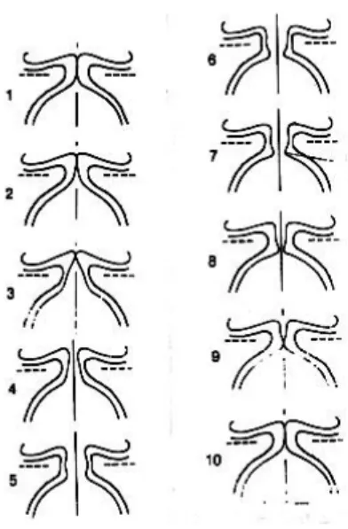
Figure 3: When air is forced up the trachea from the lungs, at a certain pressure it is able to force its way through the vocal folds, pushing them open (2, 3 and 4). As air passes through the glottis, the air pressure in the glottis falls (Venturi tube effect & Bernouilli principle) and

the vocal folds snap together, at the lower edge first, closing again (6-10). The cycle then repeats [4].

(6)

6

2 Methodology & Case-setup

The problem is to examine a simplified model of the vocal folds by Computational Fluid Dynamics (CFD) simulations using the fluid structure interaction in multiphysics tool COMSOL [5]. The problem was further divided into two parts; fluid structure interaction with one flexible obstacle and later on simulating two flexible obstacles representing the vocal folds. Thebehavior of the folds was studied by changing few parameters; Reynolds number, Young’s Modulus & Glottal-gap. Boundary conditions were set and grid

resolution-study was conducted in order to carry out an accurate study.

2.1 Solver Characteristics

Fluid Structure Interaction (FSI) is used to study and solve for flow in a continuously deforming geometry. A flexible obstacle is placed in a channel where airflow is from left to right implying load on the obstacle. The structure and material of the obstacle allows it to deform under applied force, which changes the geometry and flow in the channel. This is called two-way coupling where the flow affects the obstacle and vice-versa.

The flow is described by the incompressible Navier-Stokes equations for fluid mechanics (1) below.

[ ( ( ) )] (( ) ) ( 1)

Where u=(u,v) is the velocity field, p is the pressure and F is the volume force affecting the fluid, which is zero as no gravitation or other volume forces affect the fluid has been assumed. um is the velocity at coordinate m. The velocity profile at the inlet, uin is of a parabolic laminar character which with the steady state velocity U, can be described by (2)

√( ) ( ) ( 1)

When it comes to the structural part of the problem, COMSOL solves the deformation using an elastic and non-linear geometry formulation which allows large deformations. The object is fixed at the bottom of the channel whilst all other boundaries can deform and bend freely and experience a loaf from the fluid. To solve for the moving mesh, numerical method Lagrangian Eulerian (ALE) has been applied which helps to handle the dynamics of deforming geometry. When the obstacle deforms, new mesh

coordinates are calculated by COMSOL. The Navier-Stokes equations are solved on the freely moving mesh. The ALE method is a combination of the Lagrangian and Eulerian method. Lagrangian method solves better for mesh attached to the material while the Eulerian method is a computational system prior fixed in space. To solve for fluid structure interaction where the mesh should move with the deforming obstacle and

(7)

re-7

calculate the flow due to the two-way coupling, ALE solves the problem best. Figure 4 shows the difference between the effects of individual methods in comparison to ALE.

Figure 4: Lagrangian versus ALE descriptions. (a) initial mesh (b) ALE mesh at t=1ms (c)

Lagrangian mesh at t=1ms (d) details of interface in Lagrangian description [6].

2.2 Model Definition

Figure 5: Flow in a channel with two flexible obstacles (vocal folds)

The channel is of height 10cm, length 12cm (figure 5) with obstacle fitted to the bottom/top boundary 4mm from the inlet. The fluid is air with a density ρ=1.2 kg/m3 and dynamic viscosity µ=2·10-5 Pa·s. The obstacle is to represent the vocal folds and have therefore been given similar structures and material, but simplified. The normal density of the folds is ρ=1070 kg/m3 and the elasticity given by Young’s Modulus is E=6000 Pa [].

The characteristic of a flow in Fluid Dynamics is expressed with the help of a

dimensionless quantity Reynolds Number. This helps to compare different flows and determine the similarities between them and characterize the flow as for example laminar or turbulent. It is calculated as (3) where U is the steady state velocity.

(8)

8 ( 2) 2.2.1 Boundary conditions

The boundary conditions implied on the channel are; laminar and parabolic velocity at the inlet, p=0 at the outlet and no-slip conditions on the non-deforming walls. No-slip conditions suggest that u=0, v=0 at the walls. The velocity on the deforming surfaces’ boundaries equals to the deforming rate, default COMSOL condition).

2.3 Methods

2.3.1 Grid-resolution study

Finite Element method helps to divide the geometry in smaller elements and later on solve for the elements separately and put together their solutions. Number of mesh elements the geometry is divided into can be of a big importance as it determines the accuracy of the outcome. COMSOL uses mesh which are determined by a minimum element size, maximum element size and a growth rate. For the specific problem, minimum element size is used near the folds where we have deformation, high

velocity and pressure and with help of the growth rate the element size increases going outwards towards the inlet and outlet where we have laminar flow without

disturbances.

The project started off with a grid resolution study where the maximum element size was changed and the velocity profile for 2 different locations downstream obstacle was examined. Minimum element size and growth rate were predefined to 0.001cm and 1.3 respectively. To start off with the maximum size was set to 0.1cm which is 10% of the channel height; for laminar flows that is considered to be a finer grid. Five different grids were studied, finer to courser resolution, to observe the change in behavior of the velocity profile and determine which grid should be used for the simulations going further.

2.3.2 Glottal gap study

The vocal folds are in contact which is a significant property for the process of phonation and speech. To get a better understanding of the function, glottal gap was increased and different parameters such as velocity profile, displacement and

resistance were to be studied. The Reynolds number used during this study was 100. The model used for this project does not capture the effect of touching vocal folds due to the complexity in structure of the folds. Vocal folds in this project have been

assumed to have the same elasticity throughout and the geometry has been vastly modified. The glottal gap range used during this thesis is 4mm, 3mm, 2mm & 1mm. 2.3.3 Reynolds Number study

Reynolds number determines the flow characteristics. For sufficiently high Reynolds number, the disturbances do not resolve, vortices occur and a turbulent flow is developed. To study these effects, three different Reynolds number; 20, 50 & 100 were simulated for using the glottal gap to be 1mm. The model with one flexible

(9)

9

obstacle was even simulated for Re=500 but due to the non-availibility of resources and simplification of the vocal folds structure, same was not carried out for two flexible obstacles. A normal airflow in the vocal tract has a Reynolds number range of 100-10000.

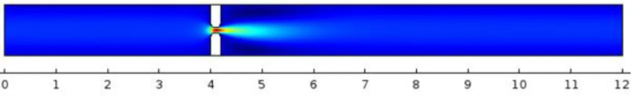
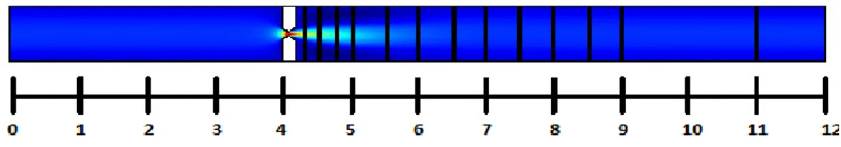
The effect of changing Reynolds number was captured by flowfield graphs to see what kind of disturbances and if any recirculation occurred. Simulations were run to plot the velocity profile at different lines downstream of the obstacle for the same different Reynolds number to compare their behavior. Figure 6 shows the different lines at which velocity profile were calculated.

Figure 6: Lines along the channel downstream of obstacle along which velocity profile were plotted.

2.3.4 Elasticity study

Elasticity explains how flexible and bendable an object is. Deciding on the Reynolds number of 100, and glottal gap 1mm; the deformation of the two folds was studied. Four different Young’s Modulus 1000 Pa, 3000 Pa, 6000 Pa (outer vocal fold layer) & 9000 Pa were tested. Displacement was plotted to study how phonation would be affected if the folds were stiffer or more flexible.

3 Results

3.1 Fluid Structure Interaction – flexible obstacle

3.1.1 Mesh Study

For the mesh study, the parameter changed was the maximum element size. The study was conducted for Reynolds number 100 and obstacle height 4.5mm. The maximum element size was increased with a factor 0.02 from 0.1cm up to the size 0.18cm. This corresponded to the total number of elements for the finest grid to be 32984 elements, maximum element size 0.1cm, while the coarser grid with maximum element size 0.18cm to have number of elements 21640. Simulation showed if increasing the maximum size resulted in the same accuracy of the result. Figure 7 and 8 shows the velocity profile for the 5 different grids along two different lines x=45mm and x=60mm on the channel. The convergence of the velocity profiles for the different grids show that the grid up to maximum element size 0.16 can provide the same result as 0.1. The velocity differs for grid 5, a negligible difference, but the variance helps in identifying the trend and seeing which grid should not be used. Using the coarser grid cuts of the simulation time but gives an uncertainty in the accuracy of the simulations,

(10)

10

specifically near the obstacle where greater disturbances appear. Therefore, the study is further carried out using the finest grid with maximum element size 0.1cm.

Figure 7: Velocity profile at x=45mm. G1 is the finest grid while G5 is the coarsest.

Figure 8: Velocity profile at x=60mm. G1 is the finest grid while G5 is the coarsest.

3.1.2 Obstacle Height Study

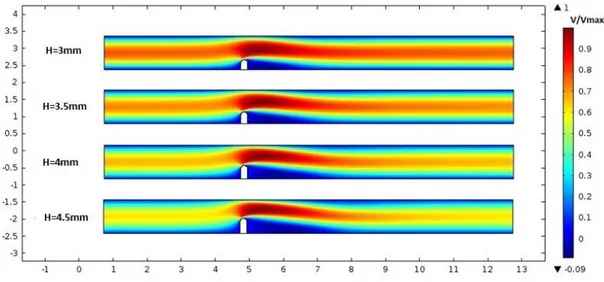
The height of the flexible obstacle was changed to observe the change in behavior of the flow. The four different heights used were 3mm, 3.5mm, 4mm and 4.5mm. A velocity flowfield was plotted for the normalized time-averaged velocities to get a better comparison of the different heights. In Figure 9 we can see the result of the simulation.

Figure 9: Normalized time-averaged velocity flowfield of the different obstacle heights at Re=100.

(11)

11

The flowfield shows how the velocity changes along the channel and where the maximum time averaged velocity is captured. For obstacle height 3mm, it is seen that there is a consistent flow where the velocity is highest near the obstacle satisfying the principles of fluid mechanics; greater velocity near smaller cross-section. The average velocity before and after the obstacle seems to be near 0.8m/s which later increases to 0.9m/s right before the obstacle followed by 1m/s on top of the obstacle. This does not correspond to a big gradient. Obstacle height 4.5mm on the other hand shows a much greater gradient where the time-averaged velocity before and after the obstacle is 0.5-0.6m/s which quickly increases to 1m/s near the obstacle. This is an indication of the increase in disturbances and instabilities near the obstacle with the increase in obstacle height.

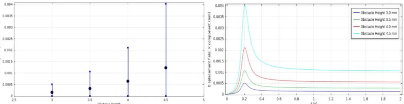
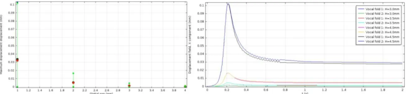
Figure 10: (Left) Time-averaged displacement represented by the black marker alongwith the maximum and minimum displacements for each obstacle height. (Right) Displacement versus

Time for the different obstacle heights.

Figure 10 shows the time-averaged as well as the maximum-minimum displacement, x-component, for the different obstacle heights and the displacement versus time graph. The minimum displacement of the structure is zero as it is taken during the steady state, when t=0. The graphs show, what looks like an exponential growth of the displacement with the increasing height of the obstacle.

3.1.3 Reynolds Number Study

The simulations conducted in this project are for a laminar velocity profile. The

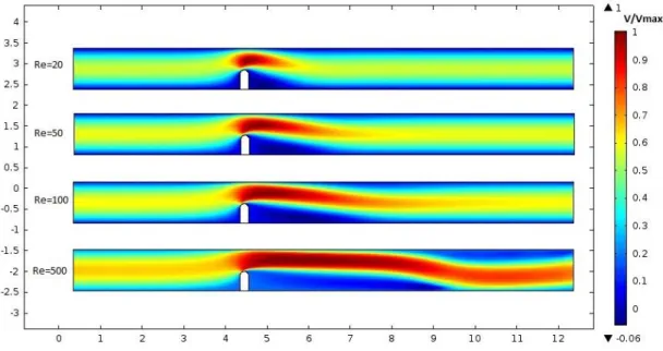
increase in Reynolds number helps to see how the disturbances start to develop. Figure 11 shows the velocity flowfield for obstacle height 4.5mm and changing the Reynolds number from 20 to 50, 100 and 500. For a low Reynolds number 20, the flowfield has a laminar flow where the velocity profile at the inlet looks exactly the same at the outlet. As the Reynolds number is increased, the flow is getting unstable. The velocity profile for Reynolds number 500 at the inlet is not similar towards the outlet of the channel. This can be solved by using a longer channel. The reattachment point is where the velocity comes in contact with the wall of the channel creating a

recirculation in the area after the obstacle and before the reattachment. It can be seen from the figure 11that the reattachment point is shifted towards the right for each increase in Reynolds number creating a longer recirculation and increased instability.

(12)

12

Figure 11: Normalized time-averaged velocity flowfield of the different Reynolds number.

Figure 12 shows the velocity field taken at different lines along the channel, at x-coordinate 43mm, 45mm, 47mm, 50mm, 55mm, 60mm, 65mm & 70mm. The velocities have been plotted at the same lines downstream obstacle to get a better comparison between the four Re. Looking at the four graphs, the velocity field does not have a parabolic profile as the

Reynolds number is increased. For Reynolds number 100 and 500, the profile is flatter which means the growth is steeper, larger gradient leading to an increased level of instability. A flat profile and large gradient are the characteristics of a turbulent flow and the graph for the different Reynolds number show that increasing the number is heading towards a more turbulent flow. The absolute value of negative velocity is also increasing with the increase in Reynolds number.

Figure 12: Time-averaged velocity versus height of the channel for lines between x=43mm & x=70mm for the different Reynolds number; 20, 50 100 & 500 respectively.

(13)

13

The time-averaged displacement and minimum-maximum displacement for the

respective Reynolds number can be seen in figure 13. Increase in Reynolds number, is giving an increase in the displacement. The maximum displacement for Reynolds number 500 is significantly larger than 20, 50 and 100.

Figure 13: Time-averaged displacement represented by the black marker alongwith the maximum-minimum displacements for the different Reynolds number.

3.1.4 Elasticity Study

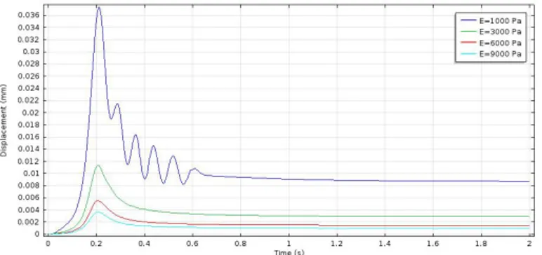
The elasticity study was conducted with obstacle height 4.5mm and Reynolds number 100. Below in figure 14 is the displacement versus time where there is a large

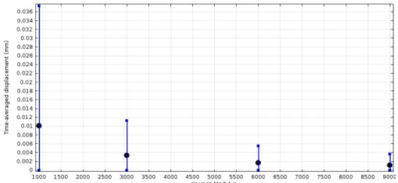
displacement for Young’s Modulus 1000Pa. There is some vibrating effect seen for the modulus of 1000. Moving towards a stiffer obstacle, 9000 Pa, there is very small displacement that has been observed. The decrease in displacement with the increase in Young’s Modulus is a non-linear decrease. The time-averaged displacement with maximum and minimum displacements is also shown in figure 15 and shows the same result.

(14)

14

Figure 15: Time-averaged displacement represented by the black marker alongwith the maximum-minimum displacements for the different Young’s Modulus.

3.2 Fluid Structure Interaction – vocal folds

3.2.1 Glottal-gap Study

For the two obstacles, representing the vocal folds, the glottal gap was altered and the normalized time-averaged velocity was simulated for. The result can be seen in figure 16. At a large glottal gap of 4mm, the profile is laminar and same at the inlet as outlet. However, at the gap of 2mm, disturbances have already developed. The velocity profile at inlet and outlet is not identical. The minimal gap used for this study is 1mm, where the velocity has large interaction with the wall. This indicates how the flow is getting instable and stating to develop turbulent characteristics.

Figure 16: Normalized time-averaged velocity flowfield of the different glottal gap at Re=100

The displacement is inversely proportional to the increasing glottal gap. The two folds have the same displacement for a larger glottal gap, but as the gap decreases; the folds get independent of each other and have a difference in the displacements. This can be seen in figure17. This independent behavior of the folds is an indication of the

(15)

15

Figure 17: (Left) Time-averaged displacement represented by the black and red marker alongwith the maximum and minimum displacements for each glottal gap. (Right) Displacement versus Time graph for the different glottal gap for the respective fold.

Pressure difference was also measure for the two folds at the entrance and exit of the fold as show in figure 18. The resulting figure shows how the pressure difference at the entrance and exit of the fold varied for the different glottal gaps. For a smaller gap, there was a significant difference between the two folds, while for a larger gap, no difference was observed.

Figure 18: (Left) The position at which the pressures are measured on the respective fold to calculate their pressure drop. (Right) Pressure difference at the entrance and exit for the

respective fold for different glottal gap.

3.2.2 Reynolds Number

The Reynolds number study is conducted for glottal gap 1mm and a laminar velocity profile is used. Reynolds numbers used for vocal folds simulation are 20, 50 & 100. The normalized velocity flowfield (figure 19) shows how the instability is captured for Reynolds number 100. There is a long interaction with the upper wall of the channel downstream obstacle. The gradient of the velocity, change in velocity near the obstacle is large for all the cases. Also, the velocity profile does not look identical at the inlet and outlet for Re=100. These are indications of disturbances in the flow due to the increase in Reynolds number. For the vocal folds’ Reynolds study, more than one recirculation was observed before the reattachment point. This can be seen in figure 20. The velocity changes the direction and this occurs due to the increase in disturbances.

(16)

16

Figure 19: Normalized time-averaged velocity flowfield of the different Reynolds number

Figure 20: Streamlines showing the recirculation bubble

The time-averaged velocity plotted for the different lines shown in figure 6 along the channel for the respective Reynolds number are shown in figure 21 below. It is of interest to observe the laminar symmetric velocity profile for Reynolds number 20. The velocity starts shifting to the right which indicates it is interacting with the upper wall of the channel and has larger negative velocity as the Reynolds number increases. For Reynolds number 100, we see the velocity does not take back its laminar parabolic velocity profile towards the outlet due to the flow taking on turbulent characteristics.

(17)

17

Figure 21: Time-averaged velocity versus height of the channel for lines between x=43mm & x=70mm for the different Reynolds number; 20, 50 & 100 respectively.

3.2.3 Elasticity Study

Figure 23: Time-averaged displacement represented by the black and red marker alongwith the maximum-minimum displacements for the different Young’s Modulus for vocal folds

(18)

18

The vocal folds are made up of three different structures all with different elasticity. The outer layer of the vocal folds is of Young’s Modulus 6000 Pa. The elasticity study is conducted to compare a stiffer obstacle as well as a more bendable obstacle with the vocal folds used in this study. For more elastic vocal folds, E=1000 Pa, the

displacement is large and the folds have displacement independent of each other, see figure 22. Some fluttering is seen in the displacement versus time graph, which takes place due to the instabilities that are occurring in the flow for a more flexible obstacle.

4 Conclusions & Reflections

Due to the advancing technology, much more is known to humans about the physiology and process of human phonation. Experimental studies are ongoing to replicate the process and discover a potential solution for people with voice disorders. However, having come a long way, there is yet a lot to be discovered to be able to completely replicate the structure and process. The biggest challenge is to model structure, material and form of the vocal folds.

The vocal folds are in contact when the air from the lungs creates a pressure forcing the folds apart, causing the self-sustained oscillations. These oscillations cannot be observed in this study due to the large glottal gap and simplification of the structure. The maximum gap, according to studies, of the vocal folds is 1mm while in this study their minimum gap is 1mm. These self-sustained oscillations are how the buzzing is produced which with the correct tongue, lips and teeth movement generate voiced speech. Though, the simulations do show the asymmetric displacement behavior of the folds for smaller glottal-gap which is an indication of the instabilities which enhance the self-sustained vibrations.

The vocal folds have a much more complex structure; they are made up of three different materials with different elasticity and behavior. These structures are not taken into account during this study resulting in the motion of the folds being far from reality. The outer folds have elasticity of 6000 Pa which is considered and thus the flapping of the folds is not observed due to this simplification. Typical Reynolds number for voiced speech lies between 100 – 10 000, which are much higher than those used in this study. Experimental studies have shown that instabilities in the human phonation CFD model, instabilities start occurring at a Reynolds number 60 which is observed in the Reynolds number study conducted. At Reynolds number 100, we had higher displacement and even larger gradient in the velocity profile. The recirculation bubbles also occurred with increase in Reynolds number, another symptom of the disturbances. Due to the time constraints of the study performed and non-availability of resources and knowledge to conduct a larger more reality-based simulation, the highest Reynolds number used for the vocal folds is 100 in this study. Higher Reynolds number would have helped in observing vortical structures downstream the folds developed due to the instabilities. The vortices in supraglottal tract in combination with the shear layer instabilities in the jet give rise to vortical structures in the supraglottal region and these structures in turn influence the glottal jet trajectory to produce sound.

(19)

19

The process of phonation is in the term of fluid dynamics, a two-way coupling process where the fluid, air from lungs, affects the vocal folds and the movement and vibrations of the vocal folds in turn affect the flow. This was taken into account during the simulations where mesh would be recalculated because of the change in flow due to the folds. This study is a simplified model of the vocaltract, however different observations and conclusions can be drawn about the behavior of the vocal folds by changing different parameters. The displacement of the folds was independent of each other with the

increase in Reynolds number, decrease in glottal gap and increase in elasticity. This shows the disturbances and characteristics of the self-sustained oscillations. The different

displacement graphs show that the growth/reduction is exponential. The other general conclusions drawn from this study are; higher Reynolds number, smaller Young’s Modulus and smaller glottal-gap giver larger displacement.

(20)

20

5 References

[1] Toward a simulation-based tool for the treatment of vocal fold paralysis, May 2011, Rajat Mittal, Zudong Zheng, Rajneesh Bhardwaj, Jung Hee Seo, Qian Xue, Steven Bielamowicz

[2] http://en.wikipedia.org/wiki/Larynx

[3]Anatomy and physiology for speech, language and hearing, 2010, 4th edition, J Anthony Seikel, Douglas W king, David G Drumright)

[4] http://www.phon.ox.ac.uk/jcoleman/phonation.htm [5] COMSOL Multiphysics, COMSOL, version 4.4

[6] Arbitrary Lagrangian – Eulerian Methods J. Donea, Antonio Huerta, J.-Ph.Ponthot

and A. Rodrıguez-Ferran

[7] Fluid dynamics of human phonation and speech, November 2012, Rajat Mittal, Byron D. Erath, Michael W. Plesniak

[8] http://www.innerbody.com/anatomy/respiratory/head-neck/larynx-superior

[9] Parallel CFD simulation of flow in a 3D model of the vibrating human vocal folds, February 2012, Petr Šidlof, Jaromír Horáček ,Václav Řidký

[10] Finite Element Modeling of Airflow during Phonation, July 2010, P. Šidlof, E. Lunéville, C. Chambeyron, O. Doaré, A. Chaigne

Fluid Dynamics of Phonation.