Studies of salt diffusion process and fluxes from seabed sediments to freshwater of the Polder reservoir

Full text

(1)Hydrology Days 2005. Studies of salt diffusion process and fluxes from seabed sediments to freshwater of the Polder reservoir Xilai Zheng1, Zengwen Gao, Junwen Wu Department of Environmental Engineering, Institute of Environmental Science and Engineering, Ocean University of China. Abstract. Based on field investigation and drilling, three kinks of original, disturbed sediments and local surface water were sampled near the Muguandao Polder Reservoir. Then, the temporal-spatial varieties of salinity in fresh water and pore water were measured carefully with conductivity apparatus using column and tank tests. At last, the salt fluxes released from the deposits were calculated. This research lays a scientific foundation for the evaluation and prediction of water quality of the impounding reservoir. According to the column tests, it has been found that a 7.5cm highly concentrated salinity layer is formed above the watersediment interface due to molecular diffusion. However, salt concentration above the layer is relatively low and even. In addition, the column tests also show that salt discharge fluxes of silty clay, medium-fine sand and pelitic silt can be expressed as a negative exponential function. On the other hand, tank tests indicate that wind may influence the salt stratification above the interface, which is favorable to the salt mixture in the reservoir. Key words: water-sediment interface; salt diffusion; polder reservoir. 1. Introduction With the rapid urban outspread and high population growth rate, water shortage has become a key factor for the sustainable development of economy and society in Qingdao, China. Building polder reservoirs in the coastal regions has becoming a popular approach to solve the problem. In order to meet the demand of water in Qingdao, the Muguandao polder reservoir is to be built in the southwest of the Jiaonan County and at a small bay near the Henghe Estuary. It will intercept the surface water from the Baimahe River, Jilihe River, Henghe River and Tianshuihe River, and the catchment area of the reservoir is about 848 km2. The reservoir will occupy 25 km2 of sea bay; its average bottom elevation, water level and water depth are –3.5 m, 4.0 m and 7.0 m, respectively. According to the drilling data from 14 holes, the bottom deposits consist of silty clay, medium-fine sand and pelitic silt (Figure 1). This area has a coastal and seasonal wind climate in the warm temperate zone. Annual average precipitation is 802.9 mm and 70.1% of the rain falls in the period of June to September each year. Annual. 1. 1 Institute of Environmental Science and Engineering Qcean University of China Yushan Road 5, Qingdao 266003 P. R. China Tel: 0086-532-203-1759 e-mail: zhxilai@ouc.edu.cn. ©Hydrology Days. 237.

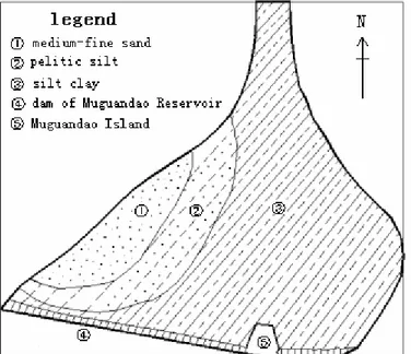
(2) Zheng et al.. average temperature and evaporation capacity are 12 °C and 960 mm, respectively.. Figure 1. Sediment distribution in the Muguandao Reservoir. Zhang et al., (1999) pointed out the water salinity in the polder reservoirs mainly depended on the disposal effectiveness of residue seawater and the salt release fluxes from seabed deposits to freshwater through molecular diffusion during the early years after a reservoir is completed. It was reported that local precipitation, evaporation and penetration through built dams also influence the salt concentrations in the reservoir (Kun 1996). Zhu (2002) pointed out water salinization in the Huchengang Polder Reservoir, China, was mainly resulted from seawater infiltration through the control gates and seawater entrance when the ship lock works. Jonathan et al. (1985) proposed an ideal model, in which water input equals to water output, to calculate the distribution of salt content in the Sungei Seletar Reservoir. Complete mixing model and incomplete mixing model at the condition of unequal input and output were respectively used to predict the varieties of water quality in the Xuanmen Impounding Reservoir, China by Yu (1996). Software Deltf-3D was also used to study the effect of regional runoff on the desalinization of saline water in the Xuanmen Polder Reservoir (Mao et al. 1997). Besides, an observation method of fluid track line was applied to describe the flow state around pump inlet, which shows it is feasible to use pumps to extract highly concentrated water from the bottom of the reservoir (Xu et. al. 1998). Some laboratory experiments and modeling about the chemical exchange between water and lake deposits were done. The results show the exchange flux under the influence of wind is bigger than that in the quiet water circumstance Portielje et al. (1999). Fick’s First Law was also used to calculate the diffusive fluxes of chemicals between seawater and sediments from the China Sea (Song, 2003). Exchange of N, P, COD. 238.

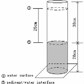
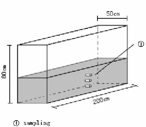
(3) Studies of salt diffusion and fluxes from seabed sediments to freshwater of Polder reservoir. and heavy metals in the Bohe Reservoir and their effects on the water quality were studied too (Lei Cui, 2003). As mentioned above, salt exchange of water-seabed sediment interface strongly affects the water quality in the early stage of a polder reservoir, but few studies have ever focused on this issue. The Muguandao polder reservoir has a big distribution area and a relatively low water depth, so it is very important to study the effects of salt exchange for the prediction of water quality verities. 2. Experimental Setups and Methods 2.1. Experimental materials and apparatuses 2.1.1 Materials. Fresh water samples are mainly from the Baimahe River, which is one of the main water sources for the reservoir. Seawater used for the tests is sampled from the nearby bay. The chemical compositions of the fresh water and seawater are shown in Table 1. Table 1. Major ions constitutes of freshwater and seawater Items. PH*. Na+. K+. Ca2+. Mg2+. Cl-. HCO3-. SO42-. Sea water [mg kg-1] Fresh water [mg kg-1]. 8.0 7.2. 7700.0 18.2. 285.0 8.7. 295.0 30.5. 922.0 21.0. 13838.0 67.9. 19.8 82.6. 646.0 50.6. *pH is no unit. 2.1.2 Apparatuses. 1. 3 plexiglass columns, 50cm high and 10cm in inside diameter, are used. Their bottoms are closed and upsides are open (Figure 2). 2. A 200×50×80 cm3 PVC water tank and an electric fan are also used for the tests. 3 sampling holes are drilled along the midline at one side of the water tank, and they are 10.0cm?19.5cm?24.5cm above the bottom of the tank respectively (Figure 3). 3. Conductivity apparatus are applied to measure the salt concentrations in water.. Figure 2. The setup of modeling column.. 239.

(4) Zheng et al.. Figure 3. The setup of experimental tank. 2.2. Experimental methods 2.2.1 Calculation of release fluxes. Conductivity apparatus DDS-11A is used to measure the water electric conductivities at different depths of the tank in the process of salt release from the seabed sediments. The salt concentration varieties in water are determined by the relationship between conductivity and salt concentration (Figure 4). In this case, the salt release fluxes (fi) at different times and the total salt release (f) from the deposits can be calculated as follows n. f = ∑ fi = i =1. ∆m i. (t i − t 0 ) × A. i = 1, " n. (1). where is the initial time for the experiments, h; is the ith hour after the experiments start, h; A is the interface area between water and deposit, m2; n is the total number of experimental periods; is the total salt charge to the water from to , which can be computed by following formula. m. ∆mi = ∑ ci j v j − c0 j v j. i = 1," n; j = 1," m. (2). j =1. where is the salt concentration of the jth water layer at the initial time, g l-1? is the salt concentration of the jth water layer at the ith hour, g l-1?is water volume of the jth layer, l?is the total number of water layers. 2.2.2 Column test. Different concentrations of sodium chloride solution are prepared and their electric conductivities are carefully measured as a standard curve. In order to get a better fitting precision, the curve is divided into two sections(Figure 4). At the beginning, three kinds of 20cm undisturbed deposits are respectively put into the perspex columns. The columns are saturated with the seawater for 32 h and then surplus seawater is sucked out.. 240.

(5) salt concentration [g L -1 ]. Studies of salt diffusion and fluxes from seabed sediments to freshwater of Polder reservoir. 1.4 (a). 1.2 1.0 0.8 0.6 0.4. y = 0.0005x - 0.0221 R 2 = 0.9993. 0.2 0.0 0. 500. 1000. 1500. 2000. 2500. salt concentration [g L -1 ]. electrical conductivity [us cm -1 ] 12.0. (b). 10.0 8.0 6.0 4.0. y = 0.0006x - 0.2416 R 2 = 0.9989. 2.0 0.0 0. 5000. 10000 15000 20000 25000. electrical conductivity [us cm -1 ]. Figure 4. Standard curves for low salinity (a) and high salinity (b) via electric conductivities. Fresh water from the Baimahe River is slowly added onto the deposits to form 25 cm water layer in the columns. Conductivity apparatuses are used to measure the electric conductivitis at 0 cm, 2.5 cm, 5.0cm, 7.5 cm, 10.0 cm 15.0 cm 20.0 cm, 25 cm above the water-deposit interface in the columns at different time intervals. In order to validate the feasibility of salty water extraction from the bottom of the reservoir, 600 ml salty water is respectively sucked out just above the interface with emulsion tubes after the tests last for 265 h. And then, fresh water is applied to compensate the extracted salty water and the tests continue. 2.2.3 Water tank test. 27.3 cm medium-fine sand and 23.6 cm pelitic silt are put into the PVC tank respectively and made them in the same bulk density as in the field. Then, the deposits are saturated with the seawater as mentioned before. The same fresh water is added to the deposits to keep 42.7 cm and 45.4 water layers above their water-deposit interfaces in the tanks. Electric fans are used to simulate natural wind. Then, electric conductivities are constantly measured at different depths along three profiles. At the same time, water is sampled with medical syringes through three sampling holes on one side of the tanks and their electric conductivities. 241.

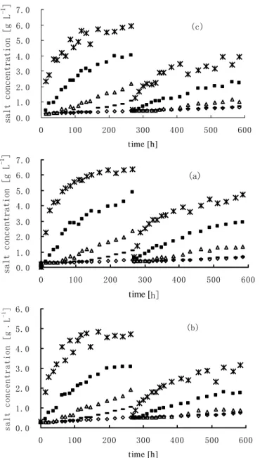
(6) Zheng et al.. are measured. The three holes are located at 4.1cm, 13.6cm, 23.6cm above the water-deposit interface. 3. Results and Discussion 3.1. Salt concentrations in fresh water 3.1.1 Change salt concentration in water for column tests. According to the measured curves for salt concentrations and electric conductivities, the salt concentration varieties at different water depths with time for 3 deposits can be presented in Figure 5?a???b???c??Figure 5(a) presents the salt concentration varieties at 0 cm?2.5 cm?5.0 cm?7.5 cm?20.0 cm above watersilty clay. The dashed line, which is parallel to the vertical axe, indicates a divergence point formed by the extraction of salt water above the waterdeposit interface so all the curves are divided into two parts. Before the extraction above the interface, the salt concentrations at different water depths increase with time, but the concentrations change slowly near the interface. At the beginning of the test, the concentrations increase rapidly at 0 cm, 2.5 cm, 5.0 cm above the interface. The salt concentration on the waterdeposit interface even arrives at 6.2 g l-1 after the test lasts for 200 hours. Then, the change rates of concentration slow down after the diffusion for a long time and the concentration curve at 7.5 cm is almost the same as that at 20 cm above the interface. This means the salt is stratified below 7.5 cm while salt concentration is relatively low and even above 7.5 cm in the undisturbed water. After the extraction from the salty water layer just above the interface, the changing trend of salt concentration in water is the same as mentioned above, but the rates of increase of the concentrations in each layer and the range of effect are smaller than before. This shows it may be feasible to extract salt water above the water-deposit interface for the desalinization of salty water in the polder reservoir. Figure 5(b) and Figure 5(c) present the same type of curves as that in Fig.5(a), but their change extent is different. Their equilibrium salt concentrations on the interface are in the order of silty clay, pelitic silt and medium-fine sand. 3.1.2 Change of salt concentration in water for tank tests. Fig. 6(a) and Fig. 6(b) present the relationship of salt concentration in water at 0 cm, 20 cm above the interfaces of water -deposits (medium-fine sand and pelitic silt). Salt concentration of medium-fine sand increases rapidly at the beginning and then stabilizes at about 1.0 g l-1 on the interface, while salt concentrations at 20 cm increase gradually (Figure 6(a)). When Figure 6(b) is compared with Fig. 6(a), it is found the varieties of salt concentration for pelitic silt are similar to medium-fine sand. However, the equilibrium period of salt release from pelitic silt is longer than that from medium-fine sand and the equilibrium concentration (1.4g l-1) for pelitic silt is higher than that for medium-fine sand. Furthermore, about 3 cm salty water layer, which is thinner than that for column test, is formed just above the water-deposit interface for both deposits. Above this layer, salt concentrations are also low and even. This shows wind has an obvious effect on salt-water mixture in a shallow water.. 242.

(7) -1. salt concentration [g L ]. Studies of salt diffusion and fluxes from seabed sediments to freshwater of Polder reservoir. 7.0 6.0. (c). 5.0 4.0 3.0 2.0 1.0 0.0 0. 100. 200. 300. 400. 500. 600. -1. salt concentration [g L ]. time [h]. 7.0 6.0. (a). 5.0 4.0 3.0 2.0 1.0 0.0 0. 100. 200. 300. 400. 500. 600. 500. 600. -1. salt concentration [g﹒L ]. time [h] 6.0 (b). 5.0 4.0 3.0 2.0 1.0 0.0 0. 100. 200. 300. 400. time [h]. Figure 5. Curves of salt concentration in water above the interface of water and silty clay (a), pelitic silt (b) and medium-fine sand (c).. 243.

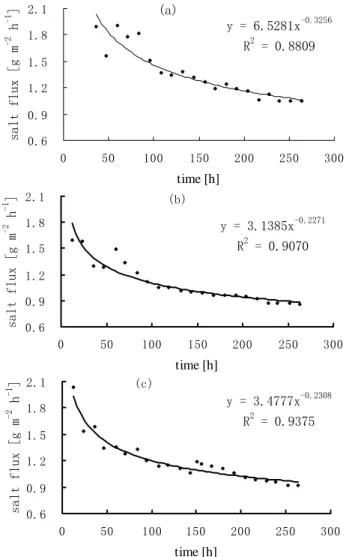
(8) -1. salt concentration [g L ]. Zheng et al.. 1.2. (a). 1.0 0.8 0.6 0.4. 20cm. 0.2. 0cm. 0.0 0. 50. 100. 150 200. 250. 300. 350. -1. salt concentratio [g L ]. time [h] (b). 1.6 1.4 1.2 1.0 0.8 0.6 0.4. 20cm. 0.2. 0cm. 0.0 0. 50. 100. 150. 200. 250. 300. 350. time [h]. Figure 6. Varieties of salt concentration in water above interface of water and medium-fine sand (a) and pelitic silt (b) in a water tank.. -1. salt concentration [g L ]. 3.2. Salt concentrations in pore water Figure 7 presents changes of salinity in pore water for pelitic silt. The salt content has an obvious drop at 4.1 cm below the water-deposit interface, while salinities only reduce slightly at 13.6 cm, 23.6 cm below the interface after 600 hours of diffusion. This shows salt release from deposit to fresh water is a very slow process? 60 50 40 30 20. 4.1cm. 10. 13.6cm. 23.6cm. 0 0. 100. 200. 300. 400. 500. 600. time [h]. Figure 7. Salinity varieties in pore water for pelitic silt. 3.3. Salt release fluxes from deposits According to column tests, salt release fluxes from deposits can be calculated by using formulae (1) and (2), and they decrease in the form of a negative exponential function (Figure 8 (a), (b) and (c)). Salt release fluxes. 244.

(9) Studies of salt diffusion and fluxes from seabed sediments to freshwater of Polder reservoir. salt flux [g m. -2. -1. h ]. reduce rapidly at the initial period of the tests, and they stabilize gradually after 200 h. Though the changing trend of salt release flux is almost same for different sediments, the release flux of medium-fine sand decrease faster than that of the other deposits and their release fluxes descend in the order of silty clay, medium-fine sand and pelitic silt. The calculation method and variety of salt release fluxes in tank tests and column tests are the same. Salt release flux of medium-fine sand is higher than that of pelitic silt. 2.1. (a). -0.3256. y = 6.5281x. 1.8. 2. R = 0.8809. 1.5 1.2 0.9 0.6 0. 50. 100. 150. 200. 250. 300. salt flux [g m. -2. -1. h ]. time [h] 2.1. (b) -0.2271. 1.8. y = 3.1385x 2 R = 0.9070. 1.5 1.2 0.9 0.6 0. 50. 100. 150. 200. 250. 300. salt flux [g m. -2. -1. h ]. time [h] 2.1. (c). y = 3.4777x. 1.8. -0.2308. 2. R = 0.9375. 1.5 1.2 0.9 0.6 0. 50. 100. 150. 200. 250. 300. time [h]. Figure 8. Varieties of salt release Flux with time for silty clay (a), pelitic silt (b) and medium-fine sand (c) 4. Conclusions 1. In the action of molecular diffusion, about 7.5 cm salinity layer is formed just above the water-deposit for different column tests, while water salinity on the upper part is relatively low and even. This means that salt in water is stratified above the interface.. 245.

(10) Zheng et al.. 2. 3 cm salinity layer (1.4g l-1) is formed above the water-deposit in tank test. Salt content above the salinity layer is also low and even. This indicates wind blowing is favorable to water-salt mixture. 3. Salt release fluxes from deposits descend in the order of silty clay, medium-fine sand and pelitic silt and they all decrease in the form of negative exponential function. 4. Salt discharge from deposit to fresh water is a very slow process under diffusion. The effect on water quality in a polder reservoir may last for 1-2 years. Acknowledgements. This research was financed by the Qingdao Water Resources Bureau. Thanks Mr. Shanfu Cheng and Mr. Guifu Cheng for supplying hydrologic data in the Muguandao region. References Cui, L., Zhou, F., Xu, J., 2003: Experimental studies of effects of deposits from an reservoir on water quality at the beginning of impoundment. J. Beijing Normal University. 39?5?, 688-693? Jonathan, A. F.?Brendan, M. H., Neysadurai, A., 1985: Desalination of an impounded estuary. Environmental Engineering. 47, 91-97. Mao, X., Chen, F., Yu, Q., 2003: 3-D stratification modeling for water desalination in a polder reservoir. International Conference on Estuaries and Coasts, Hangzhou, China: 822-828. Portielje, R., and Lijklema, L., 1999: Estimation of sediment-water exchange of solutes in Lake Veluwe?the Netherlands?J.?ater Research. 33(1), 279-285? Song, J., 1997: Chemistry of seawater-deposit interface in the China offshore. Marine Publishing House, Beijing. 56-68. Wang, G., Zhu, J., 1997: Salty water drainage and economic analysis for an impounding reservoirs. J.Zhengjiang Hydrotechnics (3), 23-25. Xu, Y., Li, M., 1998: Studies of salty water drainage in the coastal impounding reservoirs. J. Hehai University. 26(5), 76-80. Yu, K., 1996: Analysis and prediction of water desalinization in the Zhejiang impounding Reservoir.J. Environmental Pollution and Treatment. 8?2?, 27-29. Zhang, A., Zhao, Q, Jiang, Z., 1999: Prospective prediction of building up impounding reservoirs. J.Shandong Hydraulics, (6), 29-30. Zhu J., 2002: [3] Reason analysis and treatment countermeasures of water desalinization in the Huchengang impounding Reservoir.J.Zhengjiang Hydrotechnics, (4), 50-51.. 246.

(11)

No results found