AERODYNAMIC IDENTIFICATION AND MODELING OF GENERIC UCAV CONFIGURATIONS WITH CONTROL SURFACE
INTEGRATION by
JACOB DANIEL ALLEN
B.S., University of Colorado Colorado Springs, 2017
A thesis submitted to the Graduate Faculty of the University of Colorado Colorado Springs
in partial fulfillment of the requirements for the degree of
Master of Science
Department of Mechanical and Aerospace Engineering 2017
This thesis for the Master of Science degree by Jacob Daniel Allen
has been approved for the
Department of Mechanical and Aerospace Engineering by
Andrew Ketsdever, Chair
Mehdi Ghoreyshi
Julie Albertson
Allen, Jacob Daniel (M.S., Mechanical Engineering)
Aerodynamic Identification and Modeling of Generic UCAV Configurations with Con-trol Surface Integration
Thesis directed by Professor Andrew Ketsdever ABSTRACT
As aircraft are increasingly specialized for low-observability and maneuverability, the aerodynamic identification process has become increasingly important. Recently, the aerodynamics of Unmanned Combat Aerial Vehicle (UCAV) configurations have been of interest. Two UCAV designs of the same planform were the subject of this research. Techniques for aerodynamic identification were explored using data gen-erated by computational fluid dynamics (CFD). The Kestrel CFD solver was used to execute prescribed motion maneuvers, which simultaneously excite multiple flight parameters including inboard and outboard control surface deflection. The executed maneuvers are orthogonal Schroeder frequency sweeps covering reduced frequencies from 0.0069 to 0.075, superimposed with a linear Mach increase from 0.1 to 0.9. Quasi-steady aerodynamic models were developed for the longitudinal aerodynamic coefficients from the CFD maneuver data. These models are multivariate polynomial equations, developed by power series expansion of the terms of a traditional linear aerodynamic model. Additionally, a host of static, dynamic, and doublet CFD studies were completed to generate validation data to compare against the models. The mod-els showed fairly accurate matching to the static validation data, and varied force and moment predictions of the doublet maneuvers. The Schroeder maneuver required less computational resources compared to similar aerodynamic identification using current CFD techniques. Overall, the presented methods identified the aerodynamics of two UCAV configurations over a large flight envelope with reasonable accuracy, and with a 36% cost savings compared to current techniques for static aerodynamic prediction. Animations of the Schroeder maneuvers are available with this thesis.
DEDICATION
To Maggie. You’ve supported me, been patient with me, and encouraged me in every challenge I’ve faced during the last two years. I am tremendously blessed to be married to you.
ACKNOWLEDGMENTS
Many people have helped me through the process of creating this thesis. I’d like to specifically thank the members of my thesis committee: Dr. Andrew Ketsdever, Dr. Mehdi Ghoreyshi, and Dr. Julie Albertson. Having been a student to each of you at some point during my education, I know that you have fought for my academic success. I appreciate the challenges that all of you have given me, the good and bad grades, and the opportunities to learn. Thank you for choosing to share your knowledge with students like me, and for caring about our success.
Additionally, I want to thank the researchers at the High Performance Computing Research Center. Thanks to LtCol Andrew Lofthouse and Maj Matthew Satchell for answering many questions ranging from CFD to HPC access. Also, I want to thank Adam Jir´asek for the conversations about SID modeling and CFD that clarified so much for me.
TABLE OF CONTENTS CHAPTER I. INTRODUCTION 1 1.1 Motivation . . . 1 1.2 Focus . . . 4 1.3 Contributions . . . 5 II. BACKGROUND 6 2.1 Aerodynamic Modeling . . . 6 2.1.1 Aerodynamic Coefficients . . . 6 2.1.2 Traditional Models . . . 9
2.1.3 Research in Aerodynamic Modeling . . . 11
2.1.4 Computational Test Flights . . . 15
2.2 CFD Solver: Kestrel . . . . 17
2.2.1 Kestrel Infrastructure . . . . 17
2.2.2 Arbitrary Prescribed Motion . . . 19
2.2.3 Overset Mesh Simulations . . . 19
2.3 UCAV Test Case . . . 21
III. METHODOLOGY 25 3.1 Setup Details . . . 25
3.1.1 Kestrel Settings . . . . 25
3.1.2 Mesh Detail . . . 28
3.3 Validation Data . . . 33
3.3.1 Static Simulations . . . 34
3.3.2 Dynamic Simulations . . . 35
3.3.3 Doublet Maneuvers for SID Validation . . . 36
3.4 Schroeder Maneuvers for SID Modeling . . . 36
IV. RESULTS 42 4.1 Static Simulation Data . . . 42
4.2 Dynamic Simulation Data . . . 47
4.3 SID Maneuvers and Modeling . . . 53
4.3.1 Baseline Results . . . 53
4.3.2 Control Surface Results . . . 53
4.3.3 Stability Derivatives . . . 58
4.3.4 Validation Maneuvers . . . 63
4.4 Simulation Cost Comparison . . . 67
V. CONCLUSIONS 69 5.1 Completion of Goals . . . 69
LIST OF FIGURES FIGURE
1.1 A replica of the 1901 Wright Brothers’ wind tunnel (a) and lift balance (b) [3]. . . 2 1.2 The maximum speed of the fastest supercomputer in the world shown on
a logarithmic scale from 1994 to 2016. Data from Ref [5]. . . 3 2.1 The relationship between the fixed body-centered coordinate frame and
the wind coordinate frame. . . 8 2.2 The Kestrel modules shown with the option for outside modules [37]. . . 18 2.3 An example of an overset mesh showing the interpolation region. . . 20 2.4 A comparison between the SACCON and MULDICON designs [43]. . . . 22 2.5 Overhead comparison of Muld 1 (left) and Muld 2 (right). . . 23 2.6 Comparison of Muld 1 (upper) and Muld 2 (lower) from behind. . . 23 3.1 A time step comparison for CL (a) and CM (b) for a high-α dynamic
maneuver. . . 26 3.2 Visualization of the Muld 1 (a) and Muld 2 (b) meshes a different
length-wise positions . . . 29 3.3 Visualization of the Muld 1 (left) and Muld 2 (right) meshes at different
span-wise positions. . . 30 3.4 The MULDICON test points defined for AVT-251 study [43]. . . 34 3.5 The pitch doublet maneuver completed at Mach 0.5. . . 36 3.6 The control surface doublet maneuver series completed at Mach 0.5. . . 37 3.7 The simultaneous Schroeder maneuvers completed for SID Modeling. . . 38 3.8 The static regressor coverage for the SID test-flight maneuver. . . 40
3.9 The control surface deflection regressor coverage for the SID test-flight maneuver. . . 41 4.1 Streamlines over the top of Muld 1 (left) and Muld 2 (right) with no
control surface deflection at increasing Mach numbers. . . 43 4.2 Streamlines over the top of Muld 1 (left) and Muld 2 (right) with no
control surface deflection at Mach 0.4 and with increasing α. . . 44 4.3 Streamlines over the top of Muld 1 (left) and Muld 2 (right) with −20◦
IB control surface deflection at Mach 0.4 and at α = 0◦ and 15◦. . . . 45
4.4 Streamlines over the top of Muld 1 (left) and Muld 2 (right) with −20◦
OB control surface deflection at Mach 0.4 and at α = 0◦ and 15◦. . . . . 46
4.5 The change in the aerodynamic coefficients with control surface deflection compared for Muld 1 and Muld 2 and IB and OB deflections over the tested range of α. . . 48 4.6 The change in average control surface effectiveness compared for Muld 1
and Muld 2 over the tested range of α. . . 49 4.7 The longitudinal static stability derivatives calculated from static CFD
simulations over the three tested Mach conditions. . . 50 4.8 The pitching maneuver at Mach 0.8 and the regression model used to
estimate the dynamic stability derivative. . . 51 4.9 The dynamic stability derivatives calculated from pitching and plunging
maneuvers. . . 52 4.10 The SID models compared to the SID maneuver CFD aerodynamic
coef-ficient data, shown with the RMSE for Muld 1 (left) and Muld 2 (right). . . . 54 4.11 The SID model prediction of the aerodynamic impact of the control
sur-faces for Muld 1 at Mach 0.4 over at α = 0, 5, 10, and 15◦. . . . 56
4.12 The SID model prediction of the aerodynamic impact of the control sur-faces for Muld 2 at Mach 0.4 over at α = 0, 5, 10, and 15◦. . . . 57
4.13 The SID model prediction of the static stability coefficients for Muld 1 (left) and Muld 2 (right) over the tested Mach range. . . 59 4.14 The SID model prediction of the dynamic stability coefficients for Muld 1
4.15 The SID model prediction of the dynamic stability coefficients for Muld 2 over the tested Mach range. . . 62 4.16 The SID model coefficient predictions of the pitch doublet maneuver for
Muld 1 (left) and Muld 2 (right) at Mach 0.5 with ±5◦ amplitude. . . . 64
4.17 The SID model coefficient predictions of the control surface doublet ma-neuver for Muld 1 (left) and Muld 2 (right) at Mach 0.5 with ±15◦amplitude. 65
NOMENCLATURE
b Wing span
¯
c Mean chord length
CD Drag coefficient
CL Lift coefficient
Cl Yaw moment coefficient
Cm Pitching moment coefficient
CN Normal force coefficient
Cn Roll moment coefficient
CX Axial force coefficient
CY Side force coefficient
f Frequency
k Reduced frequency
M Mach number
ˆ
q Pitch rate
q Normalized pitch rate
S Characteristic area
t Time
t∗ Non-dimensional time
V Free-stream velocity
Greek
α Effective angle of attack ˆ˙α Angle of attack rate
˙α Normalized angle of attack rate
β Side-slip angle
δ Control surface deflection angle
CHAPTER I INTRODUCTION
1.1 Motivation
The aerodynamic modeling of aircraft is an incredibly complex task. Its com-plexity arises from the general comcom-plexity of fluid dynamics, which can often behave non-linearly and unsteadily even in simple cases. A well-known example of an inher-ent flow instability is the Von K´arm´an vortex street [1], which is a periodic shedding of vortices that can induce force oscillations on an object. It is well-documented in the case of two-dimensional flow past a cylinder. Aerodynamic designs are more complex, and with this added complexity comes new non-linear flow behaviors. As aircraft are designed to push the boundaries of maneuverability while striving for low-observability, it is vital to understand the aerodynamic impact of each design decision. Stability and controllability are of primary interest because these factors will ultimately determine an aircraft’s maneuverability, flying qualities, and safety.
Aerodynamic identification and modeling are an important part of the aircraft design process. Not only are late-term aerodynamic issues dangerous for test pilots, but they require costly fixes and redesigns which take time and can hamper overall aircraft performance. Wind tunnel tests have historically been used for aerodynamic identification because they can catch aerodynamic problems before full-scale flight tests are conducted. More recently, computational tools have been introduced which perform similar aerodynamic tests, but in a virtual domain. When implemented early in the process, these tools can increase efficiency and safety by identifying poor aerodynamic behavior.
The pioneers of powered flight conducted their own aerodynamic identification studies in 1901. The Wright Brothers designed and built a wind tunnel to complete airfoil testing after unsatisfactory glider tests left them questioning the data used in
(a) (b)
Figure 1.1: A replica of the 1901 Wright Brothers’ wind tunnel (a) and lift balance (b) [3].
their aerodynamic calculations [2]. The tunnel was fairly simple with an upstream fan that blew air into a square test section at speeds up to 35 mph. A mechanical lift balance was used to take measurements, shown in Figure 1.1 [3]. The Wright Brothers conducted extensive studies on more than 30 airfoil designs, which contributed to their successful 1903 flight in Kitty Hawk [2].
Wind tunnels are somewhat ill-suited for the early aerodynamic identification of complex modern aircraft. For one, design changes can happen quickly, requiring new designs to be fabricated and tested. This process is time-consuming and expensive as design iterations are made. An additional complication is that spatial and mea-surement limitations require that tests be almost exclusively static. Most dynamic maneuvers are difficult if not impossible to test in a tunnel [4]. Occasionally, tests can be completed where a design undergoes simple oscillations in pitch, roll, or yaw, which gives information about the model’s dynamic behavior. However, these test are even more time-consuming and difficult to execute than static tests. Yet, a thor-ough understanding of an aircraft’s dynamic behavior is required to analyze highly maneuverable aircraft. Another issue is that results from scale models tested in a wind tunnel can be different compared to full-scale designs, called scale effects [4].
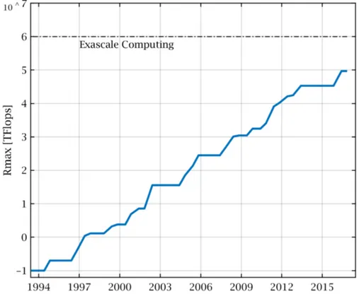
Given these limits, new technologies are under development that can reduce the need for physical wind tunnel testing. Computational fluid dynamics (CFD) is one. CFD is the numerical estimation of fluid flow in a finite, discretized spatial domain. CFD has existed in primitive form since the 1950s. The earliest methods were fairly inaccurate and the fidelity of the computational models was limited by the size and processing speed of the computers of the time. Since then, significant advances have been made in both computational capacity and processing speed. Even more re-cently, high performance supercomputing systems are on track to reach “exascale” performance, or 1018 floating-point operations per second (Flops), shown in Figure
1.2. These advances are allowing CFD and other computational engineering tools to be increasingly incorporated into mechanical and aerodynamic design processes.
Figure 1.2: The maximum speed of the fastest supercomputer in the world shown on a logarithmic scale from 1994 to 2016. Data from Ref [5].
allows any physical constraints to be avoided. Costs accrue in other areas as super-computers are needed to perform the immense number of calculations necessary in CFD simulations. Within the U.S. Department of Defense, supercomputing resources are allocated in chunks of CPU hours annually. Each simulation uses a portion of these hours, so cost is measured by the number of CPU hours per simulation.
Efforts to reduce CFD costs must focus on reducing the computational require-ment of simulations. There are numerous factors that impact the computational requirement, but the two primary factors are the spatial discretization (the mesh), and the temporal discretization (time-stepping scheme). However, these two factors are also the primary drivers of the accuracy of a computational estimation. Find-ing the proper balance of accuracy and computational cost is the challenge in usFind-ing CFD or any other computational engineering tool. The proper balance is problem dependent.
Much of the current research in reducing CFD costs focuses on the nuances of the methodologies used. For example, some simulations apply automatic adaptive mesh refinement (AMR), which refines the mesh according to certain flow values while a simulation is running [6]. Practically, this means that the mesh is refined in areas where it is most needed, and coarsened where it is not. Other techniques are being applied as well, including mixed fidelity models and reduced order models (ROMs), which allow less simulations to be completed while maintaining high accuracy. This research demonstrates a method to develop a reduced order model for aerodynamic identification using data gathered by CFD.
1.2 Focus
The focus of this thesis is to demonstrate a technique to more efficiently iden-tify and model aerodynamics of two UCAV designs across changes in Mach number, angle of attack (α), pitch rate (ˆq), and control surface deflections. The developed aerodynamic model can then be used to predict the UCAV aerodynamic behavior
through arbitrary maneuvers, offering the ability to compare aerodynamic impact of their design differences. The potential benefit is that predicting and modeling aero-dynamics using these new techniques may require less time to compute as compared to identification using more standard CFD methods, which were used to develop the validation data for this work.
The specific research goals are:
1. Use a mulivariate polynomial function for aerodynamic modeling and identifi-cation over a large flight envelope, while maintaining estimates of the static and dynamic stability derivatives after differentiation.
2. Use CFD “test-flights” to excite a large regressor space, including control surface deflections, for aerodynamic model development.
3. Analyze the accuracy of these modeling techniques compared to CFD-generated validation data.
4. Compare the time-cost of these modeling techniques with the time-cost of sim-ilar aerodynamic prediction using standard CFD methods.
1.3 Contributions
This thesis offers a few unique contributions to the field of aerodynamic modeling. Firstly, the aircraft studied in this thesis are under development and have not been studied extensively. As such, the aerodynamic results presented here are beneficial for understanding these new designs. Secondly, performing an assessment of an aircraft’s stability derivatives as well as its control surface effects over its operating Mach range using a single test flight maneuver has not been previously demonstrated. Thirdly, the aerodynamic models developed in this work will necessarily recover the stability derivatives, which is not always the case with the other polynomial models that are used currently. The stability derivatives are useful for understanding basic aircraft stability behavior.
CHAPTER II BACKGROUND
2.1 Aerodynamic Modeling
Aerodynamic modeling is of significant interest in flight dynamics. Flight dynam-ics seeks to identify the changes in overall position and velocity of an aircraft with time. This is done by developing an aircraft’s equations of motion, which relate an aircraft’s state variables to its position and velocity. The equations of motion are used to develop the models for flight computers or autopilot systems, and they are also used to test aircraft performance, including aircraft stability and control (S&C) and structural loads. Fundamentally, these equations of motion are none other than F = ma, or its rotational counterpart. However, one challenge in developing the equations of motion is determining the aerodynamic forces and moments that the aircraft experiences during flight [7].
The forces and moments that an aircraft may experience at any possible flight con-dition result from the unique fluid mechanics around the aircraft at that concon-dition. As such, these values are dependent on many variables and can behave non-linearly and unsteadily even during apparently steady flight conditions. Thus, some simplifi-cations must be made to reduce the complexity of modeling the aerodynamic forces and moments.
2.1.1 Aerodynamic Coefficients
Six aerodynamic forces and moments associated with an aircraft’s six degrees of freedom can fully define its aerodynamics. The forces are usually characterized as Lift (L), Drag (D), and Side Force (Y ), and the moments are characterized as Roll (L), Pitch (M), and Yaw (N). Traditionally, the forces and moments are non-dimensionalized so they can be directly compared between different aircraft. The longitudinal aerodynamic coefficients, which are defined in the longitudinal symmetry
plane, are Coefficient of Lift, Coefficient of Drag, and Pitching Moment Coefficient, given by: CL = 2L ρV2S CD = 2D ρV2S Cm = 2M ρV2S¯c (2.1)
where ρ is the density, V is the free-stream reference velocity, S is the characteristic area (usually planform area), and ¯c is the mean aerodynamic chord length. The lateral direction coefficients are Coefficient of Side Force, Yaw Moment Coefficient, and Roll Moment Coefficient, given by:
CY = 2Y ρV2S Cℓ = 2L ρV2Sb Cn= 2N ρV2Sb (2.2)
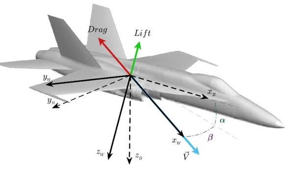
where b is the aircraft span, which is the characteristic length in the lateral direction. One important note is that lift and drag are defined in the wind coordinate system. The wind coordinate system is a rotation of the fixed body coordinate system through angle of attack and angle of side-slip as shown in Figure 2.1. Drag is the force in-line with, but opposite to, the aircraft’s velocity vector in the xW direction. Lift is
its orthogonal counterpart opposite to the zW direction, and normal to the velocity
vector.
From a flight dynamics perspective, it is often necessary to convert the aerody-namic coefficients from the wind coordinate frame to the fixed body-centered coordi-nate frame, which is completed using the following rotation:
CX CY CN =
cos α cos β 0 − sin α
0 1 0
sin α cos β 0 cos α CD CY CL (2.3)
The terms CX and CN are called the Axial Coefficient and Normal Coefficient,
and are used instead of CL and CD in this work. The aerodynamic side force in the
Figure 2.1: The relationship between the fixed body-centered coordinate frame and the wind coordinate frame.
not commonly used, but rather its fixed body frame counterpart, CY, is often used
regardless of which frame is under consideration. Thus, its transformation is unity in Eq. 2.3. The simulations in this research do not deal with side-slip angle, β, which simplifies Eq. 2.3 to a single rotation through angle of attack about the yB axis.
It is also common to non-dimensionalize the aircraft parameter rates, such as ˆ˙α and ˆq, and any others. This is done in order to eliminate any units from these values because they are commonly used in aerodynamic coefficient models which are themselves non-dimensionalized. The variable rates ˆq and ˆ˙α are non-dimensionalized by:
q = q¯ˆc
2V ˙α =
ˆ˙α¯c
2V (2.4)
While the non-dimensionalization accounts for some of the effects of changing conditions over the flight envelope, the aerodynamic coefficients can still show dra-matic changes as Mach number increases, especially over a supersonic range, due to
compressibility effects [4]. Since the non-dimensionalization doesn’t account for these variations, models are used instead to capture the compressibility effects.
Traditionally, models are developed as functions of only a few specific parameters, which have been determined through historical experience and testing. However, models exist with forms than can range from time-dependent and non-linear to quasi-steady and linear. Quasi-quasi-steady models are likely the most-used in flight dynamics because they lend well to analyzing the S&C of aircraft. A thorough discussion of aerodynamic coefficients and equations of motion is given in Refs. [4] and [7].
2.1.2 Traditional Models
The aircraft aerodynamics are commonly modeled using a quasi-steady, linear aerodynamic model. The quasi-steady assumption means that the transient effects are assumed to be immediately advected into the flow. The result is that the aero-dynamic coefficients are not directly dependent on time. This assumption is not physically accurate, but it is useful and mathematically accurate for small flow per-turbations and low frequency variations. For reference, the traditional quasi-steady, linear aerodynamic model for the Normal Coefficient is given by:
CN = CN0 + CN α∆α + CN ˙α˙α + CN qq + CN δi∆δi (2.5)
where V is velocity, α is angle of attack, q is pitch rate, and δi is the deflection angle
of the ith control surface. Similar equations are developed for the other longitudinal
coefficients, Cm, CX, and the model is modified in the relevant state variables for
the lateral coefficients. Fundamentally, this model is developed by expanding the aerodynamic coefficients using a Taylor series with respect the relevant variables and variable rates. For the linear model, the Taylor series is truncated at a first-order approximation. Consequently, each coefficient parameter, CN j, corresponds to the
As an example: CN ˙α = ∂CN ∂ ˙α ref (2.6) The Taylor series coefficients associated with the parameters α, V , and δi are
referred to as the static stability derivatives (or controllability derivatives in the case of δi), and the Taylor coefficients associated with the rates of the parameters, ˙α and q,
are called the dynamic stability derivatives (sometimes these are referred to as force-rotary or moment-force-rotary derivatives depending on which aerodynamic coefficient is studied). These are called stability derivatives because they can be used to analyze the aerodynamic stability of aircraft.
The linear aerodynamic model does a good job capturing major variations in the overall aerodynamic coefficients with respect to angle of attack, and it gives a good approximation of some of the common aerodynamic hysteresis behaviors through the inclusion of the dynamic stability terms. However, the values of the stability terms themselves are subject to the same compressibility variations with airspeed [4], and are sensitive to the flow dynamics at high angle of attack (high-α) conditions. For some aircraft these issues are never a concern if the aircraft’s flight envelope is small enough. However, the variations are of primary concern for military fighters and other aircraft that commonly deviate from trimmed flight.
Some strategies exist to account for these changes. One strategy is to develop look-up tables with the tabulated stability derivative values at discrete points across the spectrum of possible flight conditions, which allows for more accurate values to be used in Eq. 2.5. Another option is a multivariate mathematical model that is valid over the flight envelope of interest, and is a function of the relevant flight parameters. Evaluating the model at the specific flight conditions yields the pertinent aerodynamic coefficient values. Additionally, a model can be differentiated according to Eq. 2.6 to recover a function for the stability derivatives over the tested flight envelope. These models have wider application than look-up tables but can be difficult to develop.
2.1.3 Research in Aerodynamic Modeling
There is a significant body of research on methods for creating aerodynamic mod-els. Aerodynamic modeling is often referred to as aircraft system identification (SID), and falls under the field of reduced order modeling, which in general seeks to reduce the number of degrees of freedom in a model. Aerodynamic models can be developed in the temporal or frequency domains, and can be quasi-steady or fully unsteady. Additionally, they can be developed to model both the linear and non-linear regimes. When the term “non-linear” is used, it refers to the behavior of the aerodynamic sys-tem, meaning that the forces experienced by the aircraft do not behave proportionally compared to the changes in flight parameters. The models used even for non-linear modeling are mathematically linear in nature, either linear regression or linear combi-nations of basis function and weights which both rely on the superposition principle. The following is a survey of the most significant recent aerodynamic model research. Possibly the most popular quasi-steady, non-linear modeling work is that of Morelli, who authored a MATLAB package called System IDentification Programs for Air-Craft (SIDPAC) [9]. The aerodynamic models presented by Morelli are based on lin-ear regression. However, parameter selection techniques are used to select the most influential candidate regressors which are developed from combinations up to some truncated order of the physical flight parameters (α, q, etc.). These flight parameters are turned into multivariate orthogonal functions (MOF) through the Gram-Schmidt process for orthogonalization. These orthogonalized functions can then be analyzed for their respective correlation to the data, and the most significant ones are kept. An optimized model is developed based on the predicted squared error. Once the optimized number of orthogonalized functions are selected, they can be decomposed back into their original parameters to create a regression model based on the most significant combinations of these parameters. Klein and Morelli thoroughly outline this technique in Ref. [8], and it is summarized in Ref. [10].
Morelli demonstrated the MOF modeling technique by developing a series of mod-els for the aerodynamics of the F-16 [11], including control surface deflections, using data from a wind tunnel test. Additionally, Morelli used MOF models for the aero-dynamics of the T-2 subscale jet transport aircraft using flight test data [10]. The developed MOF models showed reasonably accurate prediction of a separate flight test maneuver with doublet excitations in elevator, aileron, and rudder. Additionally, Morelli and Klein demonstrated good results using MOF models on wind tunnel data of the Free-flying Aircraft for Sub-scale Experimental Research (FASER), showing how this type of model can be developed from sizable aerodynamic tables, and once developed can be used in lieu of tables [12]. MOF models are often preferable to tables because an algebraic form is easier to use for S&C analyses, and other studies. The SIDPAC program has seen wide adoption in the S&C field, and has been used in modeling wind tunnel data, flight-test data, and CFD data. Experimentally, Shepherd et al. performed an analysis on data gathered from a flight test of the T-38 Talon aircraft at multiple conditions around its flight envelope, using MOFs generated in SIDPAC [13]. The models developed showed good matching of the measured flight test data. However, the aerodynamic models were developed at the specific flight conditions where the tests were conducted, and no models were developed to interpolate between the conditions.
The application of MOFs to CFD data has been more widespread compared to wind tunnel and experimental data. Dean, Morton, et al. constructed aerodynamic models for the F-16C using data from time-accurate maneuver simulations using the Cobalt flow solver, achieving good accuracy compared to Lockheed Martin’s Aircraft Trim, Linearization and Simulation (ATLAS) aerodynamic database, as well as to flight test data [14]. Dean, Clifton, et al. later used Kestrel v1.0 to show the feasibil-ity of the MOF model in capturing the aerodynamics of the F-16C [15], and somewhat so for the F-22, for which the simulation results from Kestrel v1.0 did not compare
well to those from Cobalt and ATLAS. Clifton, Ratcliff, et al. used MOFs to model the aerodynamics of the A-10C and the F-16 JSOW configuration, and showed good model prediction of separate static CFD simulation data for the A-10C [16]. Addi-tionally, the F-16C model was shown to predict with fair accuracy the reductions in directional stability resulting from the JSOW configuration.
MOFs were also used by Jir´asek and Cummings to analyze the aerodynamics of the X-31, comparing the overall modeling results between data collected using CFD solver Cobalt and wind tunnel data [17]. They identified that the quasi-steady models perform much better after high frequency data is filtered out, and also showed how an aerodynamic model can be fit to high-frequency data to give an estimate for the unsteadiness present in a flow. More recently, Morton and McDaniel used MOFs to identify the aerodynamics of the F-16XL from CFD data generated in Kestrel, and found good model prediction in CL and CY, and less so in CD and CM [18]. They also
performed a similar analysis on the flow uncertainty by fitting different MOFs to a running maximum window filter of the CFD-vs-SID error residual. This uncertainty model showed good prediction of unsteadiness in the CFD data.
Jir´asek et al. simulated a NACA0012 airfoil in Cobalt and modeled the aerody-namic results using the same technique [19]. In this study Jir´asek et al. compared different CFD maneuvers for their fit quality. Similarly, in his thesis, Butler used the MOF technique to develop models for aerodynamic identification of the F-16C, with good success [20], while comparing maneuvers, using Kestrel v2.1.2. Research on the different maneuvers used for modeling are discussed later.
Another common quasi-steady model is the radial basis function (RBF). RBFs are based on interpolating functions of the form φ (kxnk2), where kxk2 is the
Eu-clidean norm in n space, where x = x1, x2, . . . , xn. The function φ may be any of
a number of trial functions, of which common choices are Gaussian, multiquadric, and inverse multiquadric. Different trial functions are selected based on their
inter-polating smoothness and gradients. RBF interpolation works by defining “centers” in n space at which the functions will exactly predict the data. If data sets are small enough the centers can be selected at every known data point, but often larger data sets will increase the size and complexity of the resulting function to a prohibitive size. The next step is to enforce exact interpolation of the function u, through:
u(xi) = N
X
j=1
ajφ (kxi− xjk2) (2.7)
where x are the centers. This creates a linear system where Aij = φ (kxi− xjk2),
which allows the coefficients, a, to be solved by a = A−1u. The function estimation
is then evaluated at arbitrary x by plugging in x for xi. An overview of the RBF
function technique is given in Ref. [21]. Jir´asek and Cummings also analyzed the X-31 airframe using RBF models, and showed that RBFs can have similar if not better predictive capability and accuracy compared to MOFs [17].
Neural networks have also been used for aerodynamic modeling. Neural networks are based on the biological nervous system behavior, where function is generally gov-erned by connections. In an artificial neural network, layers of “neurons” operate in parallel, each operating on a combination of every connection from the previous layer. Neurons can have different transfer function form, some common examples being logical, linear, and log-sigmoid. The network is “trained” iteratively by ad-justing the weights of each connection, often by implementing a type of automatic back-propagation method based on the error of the network’s prediction [22]. A comprehensive discussion of neural networks is presented in Ref. [22].
Marques and Anderson applied neural networks with input biases to predict time-dependent aerodynamic behavior during different maneuvers, using data from Euler CFD simulations of a NACA0012 airfoil, with good matching [23]. They identified the advantage of the network’s ability to deal with and predict the time-history of aerodynamic effects. Neural networks are also able to be applied in a quasi-steady
manner, which was studied by Dean, Clifton, et al., using RBF style transfer functions in the neurons [15]. The RBF network predicted aerodynamics with similar accuracy to the MOFs. Linse and Stengel also used neural networks for quasi-steady aero-dynamic modeling, but used infinitely differentiable transfer functions and trained the network based on errors between the base aerodynamic data and the network prediction and also between the stability derivatives and the differentiated network’s predictions [24]. This allowed for the same network to predict the static stability derivatives as well as the bulk aerodynamic behavior.
Many other methods exist for aerodynamic modeling, and many have been shown to have good predictive capability. These include indicial functions [25, 26, 27], Volterra series [28] [29], Proper Orthogonal Decomposition (POD) [30], and Har-monic Analysis [31] among others.
While the models discussed here each have their advantages and disadvantages, there often exists a trade-off between model accuracy and ease of use. The disad-vantage of many models is their complexity, which prevents them from being easily integrated into the linearized equations of motion commonly used in flight dynamics [4]. This highlights the advantage of aerodynamic models that can be easily developed and implemented into flight dynamics.
2.1.4 Computational Test Flights
Some additional research exists into the best maneuvers for data generation. As discussed previously, aerodynamic models can be developed from any type of data, CFD or otherwise. CFD shows its utility in this area by eliminating certain tions that exist in experimental studies, namely mechanical and pilot G-force restric-tions, measurement noise, pilot-actuation inaccuracy. CFD test flights can sweep precise ranges of the flight envelope with exact accuracy in the aircraft parameters and no measurement noise. This offers the ability to simulate maneuvers with low correlation between parameters, allowing for more efficient data sampling. Regardless
of the domain being tested, it is necessary that any test flight excite all the frequencies of interest [32] and cover the regressor space with adequate density [19].
Jir´asek et al. explored numerous test flights computationally, comparing factors like regressor coverage and frequency content [19]. Jir´asek et al. tested pitching and plunging maneuvers. The pitching maneuvers tested 1◦ amplitude variations in α
around α = 0. The tested pitching maneuvers included a simple chirp, an offset chirp, a series of increasing amplitude spirals of different frequencies, piecewise linear spirals, offset piecewise linear spirals, and Schroeder maneuvers. The plunging maneuvers included the Fresnel integral, integrated chirps and spirals, integrated piecewise linear spirals, and an integrated Schroeder maneuvers. Jir´asek et al. concluded that the Schroeder maneuver showed balanced frequency coverage as well as a more complete regressor coverage as compared to linear or normal chirp maneuvers.
Morelli has also worked to optimize the Schroeder maneuver with good success [33]. The maneuver is optimized specifically for simultaneous excitation in multiple state variables. Schroeder signals are created by summing together sinusoids of dif-ferent frequencies into a single signal, while the phase shift of each signal is varied in order to minimize the signal’s overall peak factor. The result is a multi-frequency signal with an approximately even amplitude [34]. Morelli extends these signals to N separate signals each exciting the same overall range of frequencies. However, each individual Schroeder motion is built from unique discrete frequencies, which renders the Schroeder signals orthogonal to each other. In this manner, N state variables can be excited orthogonally and simultaneously. Morelli demonstrated the use of Schroeder maneuvers in modeling the T-2 aircraft with good success [10].
For this thesis, Schroeder maneuvers were used to develop the computational test flights completed in CFD. These maneuvers were selected over the others discussed because they have been successfully used by many authors in literature, and they have dense frequency and regressor coverage properties. Additionally, the author has
some experience using these maneuvers for aircraft SID [35]. 2.2 CFD Solver: Kestrel
Numerous CFD solvers are commonly available, and they range in their structure and features. The simulations for this thesis were completed using Kestrel v7.0.1. In 2008 the U.S. Department of Defense (DoD) established the Computational Research and Engineering Acquisition Tools And Environments (CREATE) program to bolster the acquisition process for the military through the development of computational engineering software [36]. The Air Vehicles (CREATE-AV) portion of this program provides computational engineering software specifically to aid in the design and sustainment of fixed-wing and rotary-wing aircraft. Kestrel is the CFD software developed specifically for fixed-wing aircraft and has the capability to perform high-fidelity, full-vehicle, multi-physics analyses [37].
2.2.1 Kestrel Infrastructure
Kestrel was built with an “Event-Driven Infrastructure” which allows for rele-vant modules to be called and used when needed, illustrated in Figure 2.2. Each module performs a certain function, which allows new modules to be designed and interchanged as new capabilities are developed [38].
The Kestrel CFD (KCFD) solver module is a finite-volume, cell-centered, unstruc-tured code that uses an implicit time-stepping scheme. KCFD can solve the Euler fluid equations as well as the Reynolds Averaged Navier-Stokes (RANS) equations. Numerous turbulence models are available for use with the RANS solver, including Spalart-Allmaras (SA), Spalart-Allmaras with Rotation Correction (SARC), Shear Stress Transport (SST), as well as combinations of these with Detached Eddy Sim-ulation (DES) and Delayed Detached Eddy SimSim-ulation (DDES). The code is able to solve meshes of arbitrary element type, including tetrahedrons, prisms, pyramids, and others. Additionally, meshes with mixed cell types can be used in KCFD. The code is capable of second-order spacial and temporal accuracy [6].
Figure 2.2: The Kestrel modules shown with the option for outside modules [37]. Two components have been implemented to stabilize the KCFD computational code. The first is advective temporal damping, which artificially adds dissipation to the flow solution. This is achieved by adding the temporal damping factor to the left-hand-side matrix of the discretized implicit equations. This value can be adjusted to increase or decrease the stability of the code. If the value is too high, the solution may not fully converge, but if the value is too low, the solution may become unstable. This dissipation is especially important for solution stability when modeling flows with shocks, regions of separated flow, or significant mesh motion [6]. The second stabilizing component is startup iterations, which are used to partially converge the solution before time-accurate simulations are completed. Startup iterations allow for dissipation values to be ramped from stable but inaccurate values to less stable and more accurate values while holding the simulation time at zero. This allows the initial transients of the flow to be damped, decreasing the risk of a solution failure early in the simulation, while maintaining the accuracy of any remaining time-accurate simulations [6].
2.2.2 Arbitrary Prescribed Motion
One module of Kestrel seen in Figure 2.2 is the prescribed motion module, which allows for rigid-body translation or rotation of the computational mesh with respect to the reference flow conditions. In this manner an aircraft can be put through any arbitrary maneuver. This functionality allows for computational test flights to be simulated, but with the added advantage that maneuvers that are not flyable in reality can be studied easily. An arbitrary prescribed motion can be outlined in Kestrel by a simple text file. Kestrel can interpret a motion text file in three unique formats: rotation about Euler angles, angle-axis rotation, and basis vector specified rotation. Any of the formats also allows for translations of the mesh in the inertial frame which are defined by prescribing the absolute position of the center of rotation (COR) [6].
The values of the rotation and translation of the mesh are specified in rows, where the rows correspond to the values at sequential times. When only one row is specified corresponding to a single time, the motion is assumed to be constant to match the conditions at that time. If two or three times are specified, the motion is interpolated as linear or quadratic respectively. If more than three times are specified, then a third-order spline interpolation is used to find the motion values at simulation time steps. Lastly, if the rotation and translation values are specified at every simulation time step, the motion is fully defined and no interpolation is needed [6].
2.2.3 Overset Mesh Simulations
Kestrel can simulate control surface deflections with two different methods. One is by mesh deformation, and the other is by using overset meshes. Mesh deformation works by defining slip planes at the control surface edges. The area between the slip planes is deformed to induce control surface deflection. In a simulation with dynamic deflection, this process can become slow because the control surface mesh is re-generated at each iteration. Given the nature of the simulations in this research,
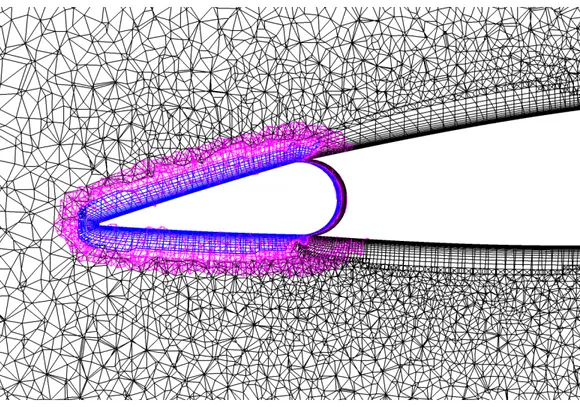
Figure 2.3: An example of an overset mesh showing the interpolation region. the mesh deformation method was not used because of the high cost of regeneration.
Alternatively, overset mesh simulation works by creating a separate mesh for each control surface. Each separate control surface mesh is cut (sub-set) to remove the majority of its surrounding flow field, such that only the mesh’s prism layers remain. The mesh is then placed inside the main aircraft mesh (overset) in the proper location. When the simulation begins, a hole-cutting algorithm selects donor cells in the main mesh from which to interpolate the flow into the control surface mesh, and vice versa. Figure 2.3 depicts the overset mesh and interpolation region after hole-cutting. The black mesh is the region of the main mesh where the flow solution is calculated, and the blue mesh is the region of the control surface mesh where the flow is calculated. The purple mesh that overlaps the black and blue meshes is the interpolation region where flow entering the overset mesh is interpolated in, and flow exiting the overset mesh is interpolated back out into the main mesh.
defines new interpolation regions at each time step. The speed of the algorithm is proportional to the number of cells over which it searches [6]. The original control surface meshes are sub-set in order to reduce the number of cells that must be analyzed at each time step, which speeds up the simulation.
2.3 UCAV Test Case
The aerodynamic designs studied in this thesis were developed under a broader research program, organized by the North Atlantic Treaty Organization’s (NATO) Science and Technology Organization / Applied Vehicle Technology (STO/AVT). Responding to the challenges in designing aerial vehicles that are highly maneu-verable but maintain low-observability, multiple NATO research collaborations have analyzed low-observability, lambda-wing unmanned combat aerial vehicle (UCAV) designs. Some research under these collaborations focused specifically on CFD flow prediction and its capabilities in the aircraft design process, and in S&C analysis.
The NATO AVT-161 Task Group developed a specific planform design, called the Stability And Control CONfiguration (SACCON). Experimental and CFD studies were conducted on this planform without any control surface integration for validation purposes [39].
The NATO AVT-201 Task Group performed more S&C analysis on the SACCON, but with control surface integration using both experimental and CFD study. Ad-ditionally, this Task Group focused on performing full flight CFD simulations [40]. One important observation from the work in AVT-201 was the lack of effectiveness of the trailing edge control surfaces because of significant span-wise flow at the trailing edge [41].
Currently, the AVT-251 Task Group is extending previous research on the SAC-CON, in order to redesign the UCAV to better meet its mission goals. The AVT-251 is studying a new MULti-disciplinary CONfiguration, the MULDICON, which has a new planform, shown in Figure 2.4. The main difference between the designs is a
Figure 2.4: A comparison between the SACCON and MULDICON designs [43]. reduction in the trailing edge sweep angle. One goal of this design change was to increase the trailing edge control surface effectiveness under high-α conditions. The integration of an engine [42] and control surfaces into the MULDICON design are being actively researched.
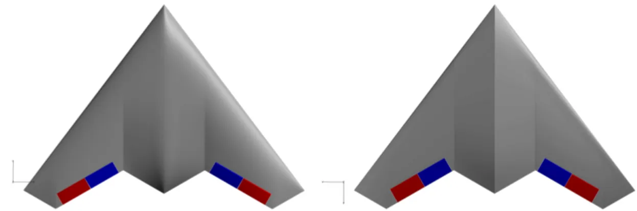
This thesis specifically focuses on the control surface integration of the MULDICON design. Two separate MULDICON designs were studied with significantly different span-wise profile shapes. The first design (Muld 1) was developed by Nangia Areo Re-search Associates and was created using an aerodynamic optimization technique. Its control surfaces were integrated and meshed at the United States Air Force Academy (USAFA). The second design (Muld 2) was developed completely at USAFA. This design used the span-wise profiles used on the SACCON, and was of interest because of the close comparison between the MULDICON and the SACCON designs. A visual comparison between the two MULDICON designs is presented in Figures 2.5 and 2.6. One important note about these designs is that Muld 1 had a scaling issue that was undiscovered until after the mesh control surface integration was completed. The Muld 1 mesh was scaled up to the full size, but the control surfaces were placed more
Figure 2.5: Overhead comparison of Muld 1 (left) and Muld 2 (right).
outboard than intended. Additionally, the overall area of the control surfaces was slightly less than that of the Muld 2 design. This difference is slight, but can be seen in Figure 2.5.
CHAPTER III METHODOLOGY 3.1 Setup Details 3.1.1 Kestrel Settings
Different solver settings were used between the static and the dynamic simulations, but both types were run as unsteady cases, with a globally specified time steps. This time step was selected based on the t∗ criterion outlined by Cummings et al. [44],
and defined as t∗ = ∆tV /¯c. A time step of approximately t∗ = 0.01 was selected for
the simulations. Physically, this means it takes 100 time steps for a particle at free-stream velocity to travel the aircraft reference length. Since the reference velocity for the dynamic simulations changes, a fixed reference velocity was selected arbitrarily at Mach 1. This is a conservative reference velocity since all simulations were completed at velocities below Mach 1, which would have corresponded to larger time steps.
Cummings et al. note that this time step does not guarantee accurate simulations, and that time step and mesh density should be selected based upon the temporal and spatial scales of the flow features which must be resolved [44]. In this case, only the bulk flow features that contributed significantly to the aerodynamic coefficients were of primary interest. The less significant, smaller-scale flow features were of less importance. As a result, reasonably dense meshes were developed, and three time steps were studied for aerodynamic coefficient convergence.
The time step study was conducted using a MULDICON mesh without integrated control surfaces, with the coarsest time step at t∗ = 0.01. A comparison between the
aerodynamic coefficients calculated during a sinusoidal motion using different time steps are shown in Figure 3.1. This figure shows that t∗ = 0.01 resolved the coefficient
values with reasonably equivalent accuracy compared to the other time steps, so this time step was used for the simulations in this work.
(a)
(b)
Figure 3.1: A time step comparison for CL (a) and CM (b) for a high-α dynamic
When solving the RANS equations in turbulent regimes, turbulence models are implemented to increase the fidelity of the simulations. In turbulent flows, fluid momentum is converted to heat energy through the development of chaotic, unsteady eddies of varying length scales. Certain turbulence models specialize in modeling turbulent effects in different flow situations. SARC+DDES was selected for the UCAV simulations because it specializes in predicting turbulent flows with large separated regions and vortices, which are common in swept-wing aircraft simulations at high angles of attack, or with significant control surface deflection. Additionally, Nelson et al. showed better matching to experimental results for the SACCON configuration using the SARC+DDES as compared to the SST+DDES model [45]. A comparison of turbulence models was not conducted in this work because no experimental data yet exists for the MULDICON design, and so there is no way to determine which turbulence model is most accurate.
Newton sub-iterations are used in Kestrel to increase the accuracy of unsteady simulations with large time steps. During each sub-iteration, an iterative solution is computed for the system matrix that results from the implicit time-stepping scheme until the convergence criterion has been reached. One sub-iteration is used for steady state simulations since the time-step is physically meaningless. Three sub-iterations are usually used for unsteady simulations or simulations with overset meshes, and 5 sub-iterations are used for simulations with mesh motion [6]. For the static simu-lations in this work, three sub-iterations were used because of the unsteadiness and overset meshes. Five sub-iterations were used for the prescribed motion simulations. A higher number of sub-iterations increases the overall simulation run-time.
All the simulations were initialized with 600 startup iterations to converge the flow before the time-accurate iterations began. Additionally, advective temporal damping values of 0.005 were used for the static simulations. The temporal damping value was increased to 0.15 for the dynamic simulations because of observed solution instability,
and total simulation failure, at values below this number. 3.1.2 Mesh Detail
Only the longitudinal coefficients were studied for this research, so half-meshes were used, symmetric along the longitudinal axis of the aircraft. The meshes were generated in Pointwise with layers of prismatic cells in order to accurately resolve the fluid boundary layer. On top of the prism layers, a tetrahedral mesh was constructed out to the hemispherical farfield with a radius of 100 m. A hemispherical refinement zone was enforced around the aircraft body with a radius of 12 m. Spacing of the prismatic layers was designed to have a y+ close to one at the free-stream conditions
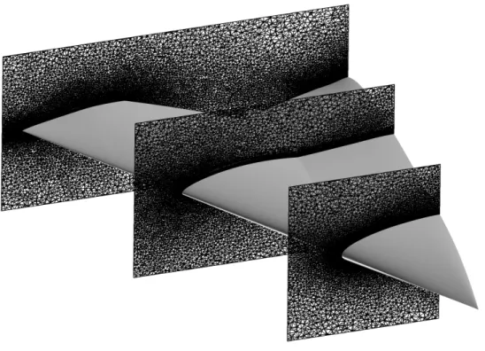
tested. The Muld 1 and Muld 2 meshes are compared in Figures 3.2 and 3.3.
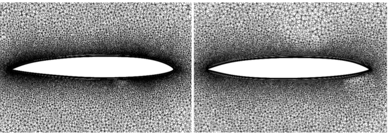
The Muld 1 mesh is more refined in the prism layers compared to the Muld 2 mesh, because the Muld 2 mesh was coarsened and re-generated after stability issues were discovered in the overset interpolation. For the purposes of this research, mesh density has little impact since the simulations used to train the models were tested against static simulations using the same mesh. Therefor, the accuracy of the modelling method is measured by the comparison between the results, not by how close the values are to reality. The Muld 1 mesh has 23,099,052 cells, and its inboard (IB) and outboard (OB) control surfaces have 887,347 cells and 793,331 cells respectively. The Muld 2 mesh has 17,566,352 cells, and its IB and OB control surfaces have 488,803 cells and 543,008 cells.
3.2 Aerodynamic Model Development
The models used in this thesis are fundamentally based on the linear aerodynamic model presented in Equation 2.5, and are designed to necessarily recover the stability derivatives that are commonly used in flight dynamics. The goal of developing the models here was to capture the UCAV aerodynamics over a large portion of the flight envelope while also maintaining some estimation of the static and dynamic stability derivatives. This derivation is completed for reference on the linear aerodynamic
(a) Lengthwise mesh profiles
(b) Lengthwise mesh profiles
Figure 3.2: Visualization of the Muld 1 (a) and Muld 2 (b) meshes a different length-wise positions
(a) Mesh at 1 meter span (b) Mesh at 1 meter span
(c) Mesh at 3 meters span (d) Mesh at 3 meters span
Figure 3.3: Visualization of the Muld 1 (left) and Muld 2 (right) meshes at different span-wise positions.
equation for CN:
CN = CN0 + CN α∆α + CN ˙α˙α + CN qq + CN δi∆δi (2.5)
Next, each CN j term is expanded using a multivariate power series expansion in M
and α, shown below for CN α:
CN α(M, α) = β0+ β1(M + α) + β2(M + α)2+ · · · + βn(M + α)n (3.1)
This equation can be expanded. Any scalar factors from the binomial expansion are absorbed into the β coefficients, and any like-terms can be combined to give:
CN α(M, α) = β0+ β1M + β2α + β3M2+ β4M α + β5α2+
β6M3 + β7M2α + β8M α2+ β9α3. . . (3.2)
Each stability coefficient in Eq. 2.5 can be expanded similarly. Many of the terms will show up twice as the different stability derivatives of Eq. 2.5 are expanded, but these can be combined to have a common fit coefficient. Additionally, the order of expansion of each stability coefficient can be varied to minimize the error of the model or to simplify the model. For example, in this work a first order approximation of the Mach and α effects was made on the CN ˙α, CN q, and CN δi terms. Third order and
fourth order Mach and α expansions were completed in CN α and CN0 respectively.
It would be feasible to develop an automatic minimization algorithm to select the expansion order truncation values, but this was not completed in this work. The final
model that was used to model the MULDICON is given by: Ca= β0+ β1α + β2α2 + β3α3 + β4α4+ β5M + β6M2+ β7M3 + β8M 4 + β9M α + β10M α 2 + β11M α 3 + β12M 2 α + β13M 2 α2+ β14M 2 α3 + β15M3α + β16M3α2+ β17q + β18˙α + β19M q + β20M ˙α + β21αq + β22α ˙α + β23δOB+ β24δIB+ β25M δOB+ β26M δIB+ β27αδOB+ β28αδIB (3.3) where a = N, m, X.
With the model in this form, the β coefficients can be solved by linear regression. In linear regression, the fitting model must be of the form:
y = β0x0+ β1x1 + β2x2+ β3x3+ · · · + βmxm (3.4)
where βi is a fit coefficient, xi is an independent variable (or regressor), and y is the
dependent variable. When data series exist for each xi and also for y, the system can
be expressed in the following form:
~y = X~β + ~ǫ (3.5)
where X corresponds to the matrix of data. This matrix has dimensions governed by the data series length, m, and the number of regressors, n, and is given by:
X= x00 x01 x02 . . . x0m x10 x11 x12 . . . x1m x20 x21 x22 . . . x2m ... ... ... ... ... xn0 xn1 xn2 . . . xnm
Minimizing the squared error allows the fit coefficients, ~β, to be estimated by:
~
β = (XTX)−1(XT~y) (3.6)
The modeling work was implemented using MATLAB. The matrix inversion in Eq. 3.6 is only n × n, which allowed normal inversion techniques to be used.
The utility of the multivariate polynomial SID model is that the static and dy-namic coefficient terms are easily recovered by differentiating the model with respect to the proper parameter, according to Eq. 2.6, and then by plugging in the reference condition at which the stability coefficient term is desired. The author developed a model using similar methodology for the identification of the static and dynamic stability coefficients for a generic missile configuration over a Mach range from 0.5 to 4.5 with good success in Ref. [35].
The reason this model was used over the MOF models discussed previously comes down to the desire for these models to necessarily recover the dynamic stability coef-ficients after differentiating according to Eq. 2.6. The MOF models do not guarantee the recovery of the dynamic stability derivatives because the automatic parameter selection can eliminate the terms associated with ˙α and q. The model presented here will always return a dynamic derivative estimate after differentiation. Another im-portant note is that this aerodynamic model is developed to be able to separate and independently model the ˙α and q effects, which are often grouped together but can have significant independent aerodynamic impact.
3.3 Validation Data
In order to compare the aerodynamic identification methods in this thesis, a set of validation data was created. The set of validation data was developed through static simulations at multiple points around the flight envelope. Additionally, some dynamic simulations were completed at different Mach numbers to show some measure
Figure 3.4: The MULDICON test points defined for AVT-251 study [43]. of accuracy of the prediction of the dynamic stability derivatives. Doublet maneuvers were also completed in pitch and in control surface deflections to have some dynamic CFD data which can be compared against SID model predictions.
The added benefit of developing this data set using current CFD techniques is that this data can be used preliminarily for AVT-251. This data can be analyzed for the desired aircraft performance as well as compared to the aerodynamics of the SACCON.
3.3.1 Static Simulations
Four test points are defined by the AVT-251 Task Group for specific study. The static simulations in this study were completed at three of these. These points are outlined in Figure 3.4. The three test points at sea-level were studied in this work.
Simulations were completed for ±10◦ and ±20◦ IB and OB deflections, including
simultaneous and cross deflections (i.e.; ±20◦ IB and ±20◦ OB, as well as ±20◦ IB
and ∓20◦OB). Additionally, four angles of attack were studied at test point two, with
in order to study the effects of angle of attack change on the control surfaces and stability derivatives. Simulations at α = 5◦ were completed with no deflection at test
points one and three to estimate the static stability derivatives at these points. The simulations were completed for 3500 iterations, and the last 1500 iterations were aver-aged to determine the longitudinal aerodynamic coefficient values at each condition. By convention, the control surface deflections are measured positive for a trailing edge down (TED) deflections.
3.3.2 Dynamic Simulations
Dynamic simulations were completed to determine the dynamic stability coeffi-cients. These dynamic simulations are oscillatory in nature, and the frequency of oscillatory motions can be non-dimensionalized in terms of the reduced frequency, given by:
k = 2πf ¯c
V =
ω¯c
V (3.7)
where f is the frequency of oscillation, and ω corresponds to the angular frequency. In order to measure the dynamic aerodynamics, oscillations are induced that excite dynamic angle of attack effects. These aerodynamics are due to the parameters ˙α and q. When α = θ, then the ˙α effects cannot be separated from the q effects. To separate these effects, two oscillatory motions are completed at each condition: a pitching oscillation and a plunging oscillation. The pitching oscillation works by prescribed mesh rotation. Translations of the mesh simultaneously maintain an effective angle of attack equal to zero. The plunging oscillation varies the angle of attack again by vertical and horizontal mesh translations within the reference flow, while maintaining the reference velocity and without any mesh rotation thereby avoiding any rotational effects.
These pitching and plunging simulations consist of a 1◦ single oscillation at a
reduced frequency of k = 0.075. This reduced frequency was selected to match the maximum reduced frequency excited by the SID maneuvers. Pitching and plunging
Figure 3.5: The pitch doublet maneuver completed at Mach 0.5.
maneuvers were completed at test points one, two, and three, shown in Figure 3.4. 3.3.3 Doublet Maneuvers for SID Validation
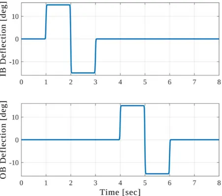
Doublet maneuvers were completed at Mach 0.5. For both MULDICON designs, a doublet simulation was performed in pitch by simple prescribed mesh rotation, shown in Figure 3.5. Additionally, a doublet series was performed for both designs with an IB doublet first and then an OB doublet, shown in Figure 3.6. The steps in these maneuvers were smoothed somewhat with a moving average filter to help with the stability of the CFD simulations. These maneuvers and conditions were selected arbitrarily, and the CFD results were compared to the SID models developed in this work to check the SID models’ predictive capability.
3.4 Schroeder Maneuvers for SID Modeling
Schroeder maneuvers were completed to generate the data for the SID models. Four Schroeder signals were created using the mkmsswp.m MATLAB function from SIDPAC [9]. The total maneuver time was 40 seconds, which was determined through
Figure 3.6: The control surface doublet maneuver series completed at Mach 0.5. the author’s experience as well as by inspecting the regressor coverage of the Schroeder signals. The Schroeder maneuvers were constructed from independent reduced fre-quencies ranging from the lower limit Nyquist frequency, k = 0.0069, up to a reduced frequency of k = 0.075. The upper level reduced frequencies are above what is usu-ally considered quasi-steady. However, the author’s experience has shown that higher reduced frequencies can be excited in a Schroeder maneuver without large deviations from quasi-steady flow. Higher reduced frequencies are allowable because the nature of the developed models is to average the aerodynamics across the many frequencies excited during a Schroeder maneuver. The models are quasi-steady so they cannot independently model lower and higher frequency effects at a single flight condition, so instead they essentially average the effects over the tested frequency range. The Schroeder maneuvers are shown in Figure 3.7
flection, and OB deflection. Exciting θ and α independently creates a data set that allows for the dynamic stability derivatives to be separated, similar to how pitching and plunging motions are traditionally completed for dynamic derivative estimation. In essence, the Schroeder signal corresponding to α is a plunging signal, and the Schroeder signal corresponding to θ is a pitching signal.
The α signal was set to cover an amplitude range from −5◦ to 15◦, which captures
the linear as well as the beginning of the non-linear angle of attack effects. Feasibly, this amplitude range in α could be increased to cover a more non-linear flight regime when needed. The θ signal was set to cover a range of ±10◦. The amplitude of
the θ signal has no physical significance, however, it was set to the same order of magnitude as the α signal to keep q and ˙α at about the same magnitude. The IB and OB deflection signals were set to cover a range of ±20◦. Again, this range could be
increased to cover larger deflections. The outlined amplitude ranges are approximate and vary slightly due of the peak factor optimization process. Additionally, the maximum control surface deflection rate was 2.51◦ per second.
Simultaneous to the prescribed Schroeder signals, a linear increase in Mach num-ber was induced by translating the mesh forward into the reference flow. The effect is that the Schroeder oscillations essentially excite the aerodynamics at close-to steady-state values at the instantaneous Mach condition, which slowly changes throughout the simulation. This technique was shown to be accurate by Morelli in the modeling of the T-2 subscale jet [10]. Morelli summarized this approach, stating:
This approach is practical because the orthogonal optimized multi-axis perturbations excite the aircraft dynamics in a very time-efficient manner with high data information content, so that the aircraft dynamics can be sufficiently excited even when the flight condition is changing [10].
The Mach condition was continuously swept throughout the 40-second maneuver from Mach 0.1 to 0.9. The author has executed Schroeder and chirp maneuvers with similar Mach sweeps to generate CFD data for SID modeling [35,42]. In the author’s
Figure 3.8: The static regressor coverage for the SID test-flight maneuver. experience, the Mach sweep should cover a Mach range beyond the limits of the data of interest, because there is limited aerodynamic information at start and finish of the maneuver. Additionally, Mach sweeps should increase in speed, not decrease, which allows the aircraft to move past any transient shocks and pressure waves generated by the maneuvers. If the aircraft is decreasing in speed, these compressive waves will pass over the vehicle and disturb the data, resulting in poor modeling. Figure 3.8 shows the static regressor coverage of the Schroeder maneuvers, and Figure 3.9 shows the control surface regressor coverage over the same period.
Figure 3.9: The control surface deflection regressor coverage for the SID test-flight maneuver.
CHAPTER IV RESULTS
4.1 Static Simulation Data
A selection of the Static CFD simulation results are presented here. Comparison between the baseline (no deflection) results at α = 0◦ is shown at the three test points
tested in Figure 4.1. These results were as expected, with no major separated flow regions. Only small wingtip vortices are apparent, and they are significantly more defined on the Muld 2 design.
The baseline results at Mach 0.4 are shown in Figure 4.2, where multiple angles of attack were simulated. The development of separated flow regions can be seen toward the wingtip of both aircraft as α increases. When these types of separated flow regions envelop a control surface, loss of control effectiveness is often observed. At α = 15◦ the separated region on the Muld 1 design is significantly smaller and
more outboard than that of the Muld 2 design. Overall, the Muld 1 design tends to develop smaller vortices and separated flow regions.
Figure 4.3 shows the results for a −20◦ IB deflection at Mach 0.4 comparing
α = 0◦ and 15◦, and Figure 4.4 shows the results for a −20◦ OB deflection. The
separated flow region in Figure 4.4 on the Muld 2 design can be seen enveloping the OB control surfaces. Additionally, this flow separation pulls the flow in a more span-wise direction at the trailing edge of the wing, and thus along the length of the OB control surface instead of directly over it. Both of these effects likely cause a decrease in control surface effectiveness.
Conversely, the IB deflection results in Figure 4.3 show that the separated flow does not envelop the IB control surface. However, the nose vortex circulatory effects and the change in stream-wise flow direction at α = 15◦ appear to negatively impact
(a) Mach 0.2 (b) Mach 0.2
(c) Mach 0.4 (d) Mach 0.4
(e) Mach 0.8 (f) Mach 0.8
Figure 4.1: Streamlines over the top of Muld 1 (left) and Muld 2 (right) with no control surface deflection at increasing Mach numbers.
(a) α = 5◦ (b) α = 5◦
(c) α = 10◦ (d) α = 10◦
(e) α = 15◦ (f) α = 15◦
Figure 4.2: Streamlines over the top of Muld 1 (left) and Muld 2 (right) with no control surface deflection at Mach 0.4 and with increasing α.
![Figure 2.2: The Kestrel modules shown with the option for outside modules [37].](https://thumb-eu.123doks.com/thumbv2/5dokorg/4336005.98438/29.918.169.806.104.461/figure-kestrel-modules-shown-option-outside-modules.webp)
![Figure 2.4: A comparison between the SACCON and MULDICON designs [43].](https://thumb-eu.123doks.com/thumbv2/5dokorg/4336005.98438/33.918.199.772.110.413/figure-comparison-saccon-muldicon-designs.webp)
![Figure 3.4: The MULDICON test points defined for AVT-251 study [43].](https://thumb-eu.123doks.com/thumbv2/5dokorg/4336005.98438/45.918.205.771.110.470/figure-muldicon-test-points-defined-avt-study.webp)