SKI Report 2005:24
Research
DECOVALEX III/BENCHPAR PROJECTS
Implications of Thermal-Hydro-Mechanical
Coupling on the Near-Field Safety of
a Nuclear Waste Repository
Report of BMT1A/WP2
Edited by:
L. Jing
T.S. Nguyen
February 2005
ISSN 1104–1374 ISRN SKI-R-05/24-SESKI Project Number XXXXX
SKI Report 2005:24
Research
DECOVALEX III/BENCHPAR PROJECTS
Implications of Thermal-Hydro-Mechanical
Coupling on the Near-Field Safety of
a Nuclear Waste Repository
Report of BMT1A/WP2
Edited by:
L. Jing¹
T.S. Nguyen²
¹Division of Engineering Geology, Department of Land and Water
Resources Engineering, Royal Institute of Technology, Stockholm, Sweden
²Canadian Nuclear Safety Commission, Ottawa, Ontario, Canada
February 2005
This report concerns a study which has been conducted for the DECOVALEX III/ BENCHPAR Projects The conclusions and viewpoints presented in the report are those of the author/authors and do not necessarily coincide with those of the SKI.
Foreword
DECOVALEX is an international consortium of governmental agencies associated with the disposal of high-level nuclear waste in a number of countries. The
consortium’s mission is the DEvelopment of COupled models and their VALidation against EXperiments. Hence theacronym/name DECOVALEX. Currently, agencies from Canada, Finland, France, Germany, Japan, Spain, Switzerland, Sweden, United Kingdom, and the United States are in DECOVALEX. Emplacement of nuclear waste in a repository in geologic media causes a number of physical processes to be
intensified in the surrounding rock mass due to the decay heat from the waste. The four main processes of concern are thermal, hydrological, mechanical and chemical.
Interactions or coupling between these heat-driven processes must be taken into account in modeling the performance of the repository for such modeling to be meaningful and reliable.
The first DECOVALEX project, begun in 1992 and completed in 1996 was aimed at modeling benchmark problems and validation by laboratory experiments.
DECOVALEX II, started in 1996, built on the experience gained in DECOVALEX I by modeling larger tests conducted in the field. DECOVALEX III, started in 1999
following the completion of DECOVALEX II, is organized around four tasks. The FEBEX (Full-scale Engineered Barriers EXperiment) in situ experiment being
conducted at the Grimsel site in Switzerland is to be simulated and analyzed in Task 1. Task 2, centered around the Drift Scale Test (DST) at Yucca Mountain in Nevada, USA, has several sub-tasks (Task 2A, Task 2B, Task 2C and Task 2D) to investigate a number of the coupled processes in the DST. Task 3 studies three benchmark problems: a) the effects of thermal-hydrologic-mechanical (THM) coupling on the performance of the near-field of a nuclear waste repository (BMT1); b) the effect of upscaling THM processes on the results of performance assessment (BMT2); and c) the effect of glaciation on rock mass behavior (BMT3). Task 4 is on the direct application of THM coupled process modeling in the performance assessment of nuclear waste repositories in geologic media.
On September 25, 2000 the European Commission (EC) signed a contract of FIKW-CT2000-00066 "BENCHPAR" project with a group of European members of the DECOVALEX III project. The BENCHPAR project stands for ´Benchmark Tests and Guidance on Coupled Processes for Performance Assessment of Nuclear Waste Repositories´ and is aimed at improving the understanding to the impact of the thermo-hydro-mechanical (THM) coupled processes on the radioactive waste repository performance and safety assessment. The project has eight principal contractors, all members of the DECOVALEX III project, and four assistant contractors from
universities and research organisations.The project is designed to advance the state-of-the-art via five Work Packages (WP). In WP 1 is establishing a technical auditing methodology for overseeing the modeling work. WP´s 2-4 are identical with the three bench-mark tests (BMT1 - BMT3) in DECOVALEX III project. A guidance document outlining how to include the THM processes in performance assessment (PA) studies will be developed in WP 5 that explains the issues and the technical methodology, presents the three demonstration PA modeling studies, and provides guidance for inclusion of the THM components in PA modeling.
This report is the final report of the first phase of the BMT1 (called BM1A) of the DECOVALEX III and its counterparts in BENCHPAR, WP2, with studies performed for re-evaluating the numerical modeling of the in-situ THM experiments at the Kamaishi Mine, Japan, during the DECOVALEX II project time, and calibrating the
computer codes applied for the next two phases of BMT1 (called BMT1B and BMT1C, respectively) of the DECOVALEX III and WP2 of BENCHPAR projects.
L. Jing F. Kautsky J.-C. Mayor O. Stephansson C.-F. Tsang January 2005 Stockholm, Sweden
Summary
This report presents the works performed for the firsty phase (BMT1A) of BMT1 of the DECOVALEX III project for the period of 1999-2002.
The works of BMT1 is divided into three phases: BMT1A, BMT1B and BMT1C. The BMT1A concerns with calibration of the computer codes with a reference T-H-M experiment at Kamaishi Mine, Japan. The objective is to validate the numerical approaches, computer codes and material models, so that the teams simulating tools are at a comparable level of maturity and sophistication in order to perform the scooping calculations defined in BMT1B and BMT1C.
Five teams participated in studying BMT1A: CNSC (Canada), JNC (Japan), IRSN/CEA (France), ANDRA/INERIS (France) and SKI/KTH (Sweden), using FEM approach except the INERIS team (Using FDM approach).
A simplified calibration test case of the in-situ experiment was proposed and defined as an axisymmetric model. The case focuses on the THM behaviour along a radial line (with a radial distance r as the coordinate) from the centre of the heater. The desired output parameters are: temperature, radial displacement, pore pressure, water content, the total radial stress and the radial and tangential strains, respectively. Time histories of these output parameters were calculated for both the heating and cooling phases.
A number of improvements to the modelling of the Kamaishi Mine heater test were suggested and tested in this study. Although the model geometry is much simplified compared to the field test conditions, improved simulation of the general THM
responses were obtained, as compared with the Task 2C results of DECOVAEX II. The measures taken for improvement were: i) Parameter changes (reduced rock mass
permeability and rock mass thermal expansion by the SKI/KTH team, and increased thermal expansion coefficient and reduced swelling pressure constant of the buffer by JNC team); ii) Inclusion of the sealing of rock fractures by penetrating bentonite by the SKI/KTH team, which can explain the uniform (axisymmetric) wetting of the bentonite; iii) An improved swelling/shrinking strain function combined with an increased thermal expansion of the bentonite giving a good match of the mechanical (stress, strain)
behavior of the buffer by the KTH/SKI team and iv) Use of higher E (Young’s
modulus) and ν (Poisson’s ratio) of the bentonite near the heater, and use of a “sealed” layer of rock around the bentonite by the CNSC team.
As a results of the above measures, the results from the simplified axisymmetric model used in the re-evaluation of the Kamaishi mine experiment showed general improvement over the original models used in the prediction phase during the
DECOVALEX II project. The calculated temperature results agree very well with the experimental values, for all teams. The results of stress and strain behaviour in the bentonite are generally improved, at least qualitatively though, with the measured results. The water content near the heater (at point 1) is relatively well predicted by all teams, although the saturation front at the bentonite/rock interface are still predicted to advance much faster than in reality.
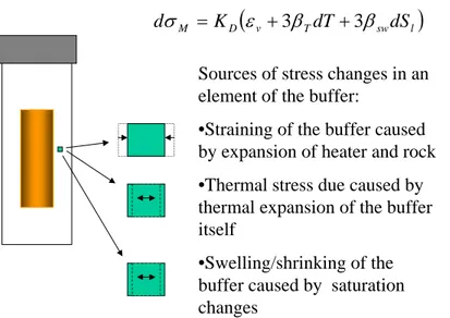
In general, the mechanical behaviour of the buffer is complex with forces
contributing from shrinking/swelling in all part of the bentonite, external stress from the thermal expansion of the heater and rock, and internal thermal expansion of the
bentonite itself. However, the BMT1A results show that a reasonable prediction of the mechanical behaviour can be done if all relevant bentonite properties are known from laboratory tests.
Content
Page
1 Introduction 1
1.1 Background 1
1.2 General definition of the problem 2
1.3 Calibration of the T-H-M experiment 5
1.4 Scoping calculations for the near-field of a generic repository 8
1.5 A simplified axisymmatric calibration case 15
of the T-H-M experiment 2 Re-evaluation of Kamaishi Mine modelling (by the CNSC team) 17
2.1 Summary of blind prediction of the Kamaishi THM experiment 17
2.2 The simplified axisymmetric model 17
2.3 Summary and conclusions 24
3 Re-evaluation of Kamaishi Mine modelling (by the JNC team) 25
3.1 Introduction 25
3.2 Temperature and density dependency of swelling pressure 25
3.3 Simulation of laboratory experiment by considering 27
The temperature and density dependency 3.4 Re-evaluation of Kamaishi THM experiment 38
3.5 Summary 45
4 Re-evaluation of Kamaishi Mine modelling (by the KTH team) 46
4.1 Suggestions for improved modelling of the Kamaishi 46
Mine heater test 4.2 A simplified axisymmetric model of the Kamaishi Mine heater test 50 4.3 Results of axisymmetric modelling of the heater test 54
4.4 Comparison of axisymmatric modelling to field observations 55
4.5 Summary and conclusions of SKI/KTH work 60
5 Evaluation of the Kamaishi Mine modelling by the INERIS team) 62
5.1 Introduction 62
5.2 Governing equations 62
5.3 Results of 1D-axisymmetric model 64
5.4 Conclusion and remarks 73
6 Evaluation of the Kamaishi Mine modelling (by the CEA team) 74
6.1 Introduction 74
6.2 Governing equations 74
6.3 Modelling data for the BMT1-A exercise 76
6.4 Results of the axisymmatric modelling of the heater test 80
6.5 Conclusion 83
7 Comparison and summary of conclusions 84
7.1 Comparison of results 84
7.2 Summary of conclusions 87
1. Introduction
1.1 Background
The DECOVALEX III project is the third stage of an ongoing international co-operative project to support the development of mathematical models of coupled Thermal (T), Hydrological (H) and Mechanical (M) processes in fractured geological media for potential nuclear fuel waste repositories. During the first stage (May 1992 to March 1995), called DECOVALEX I, the main objective was to develop computer codes for coupled T-H-M processes and their verification against small-scale
laboratory or field experiments. In the second stage, called DECOVALEX II, the main objective was to further develop and verify the computer codes developed in DECOVALEX I against two large-scale field tests with multiple prediction-calibration cycles, the pump test at the Sellafiled, UK, with a hypothetical shaft excavation and the in-situ THM experiment at the Kamaishi Mine, Japan. The third phase of DECOVALEX project, called DECOVALEX III, is initiated with two main objectives. The first is the further verification of computer codes by simulating two additional large scale in-situ experiments: the FEBEX T-H-M experiment performed in Grimsel, Switzerland, and the drift scale heater test at Yucca Mountain, Nevada, USA. The second objective is to determine the relevance of THM processes on the safety of a repository.
To achieve the second objective of DECOVALEX III project, three benchmark tests (BMT) are proposed to examine the relevance of THM processes to performance and safety assessments: 1) BMT1: the impact of THM processes in the near-field of a hypothetical repository in fractured hard rocks; 2) BMT2: homogenisation and upscaling of hydro-mechanical properties of fractured rocks and their impact on far-field performance and safety assessments; and 3) BMT3: Impact of impact of glaciation process on far-field performance and safety assessments.
On September 25, 2000 the European Commission (EC) signed a contract of FIKW-CT2000-00066 "BENCHPAR" project with a group of Europeen members of the DECOVALEX III project. The BENCHPAR project stands for ´Benchmark Tests and Guidance on Coupled Processes for Performance Assessment of Nuclear Waste Repositories´ and is aimed at improving the understanding to the impact of the thermo-hydro-mechanical (THM) coupled processes on the radioactive waste repository performance and safety assessment. The project has eight principal contractors, all members of the DECOVALEX III project, and four assistant
contractors from universities and research organisations. Kungl Tekniska Högskolan (KTH) is the coordinator of the BENCHPAR project. The project is designed to advance the state-of-the-art via five Work Packages (WP). In WP 1 is establishing a technical auditing methodology for overseeing the modeling work. WP´s 2-4 are identical with the three bench mark tests (BMT1 - BMT3) in DECOVALEX III project. A guidance document outlining how to include the THM processes in performance assessment (PA) studies will be developed in WP 5. The document will explain the issues and the technical methodology, present the three demonstration PA modeling studies, and provide guidance for inclusion of the THM components in PA modeling.
This report is concerned with BMT1 of DECOVALEX III project, which is equivalent to WP2 in BENCHPAR project. In the remaining part of this report, only the name BMT1 is used throughout for simplicity.
In the definition of BMT1, it was proposed that scoping calculations be performed in order to determine how T-H-M processes can influence the flow field, as well as the structural integrity of the geological and engineered barriers in the near-field of a typical repository. To simplify the calculation process and focus on the physics of the problems instead of computational efforts, the geometry of the problem, especially regarding the geometry of the fractures, is greatly simplified to regular fracture geometries. The problem is divided into three phases: BMT1A-calibration of numerical codes and material models according to in-situ heater experiments in Kamaishi Mine, Japan; BMT1B-coping calculations of different coupling mechanisms in continuum rocks, and BMT1C-scoping calculations of different coupling mechanisms with fractured rocks. This report is the final report for BMT1A.
1.2. General definition of the problem
The definition of BMT1 is based on a hypothetical case where one considers the feasibility of constructing a nuclear waste repository in a granitic rock formation at a depth of 1000 m. The problem is not site specific, however, in the definition of the problem, experiences was drawn from the results of in-situ tests performed at real sites, with simplified types of rock and engineered barriers. For example at one experimental site in the Kamaishi Mine, Japan, galleries were excavated down to a depth of 600 m, and a variety of hydraulic and mechanical tests have been performed (see Figure 1.1a). Of particular relevance to the assessment proposed in BMT1 is a T-H-M experiment that replicates the near field behaviour of the rock mass and buffer around a single waste container (Fig. 1.1b). The type of bentonite used in the above experiment and the dimensions of the experimental borehole are comparable with the parameters of the conceptual design.
Assume that the fracture density of the rock mass in this hypothetical case could vary with depth, with a fracture spacing of 0.1 m down to 600 m and 0.5 m at depths greater than 600 m, respectively. Based on the average properties of the rock mass determined from the site investigations, a preliminary design of the repository is proposed as shown in Figure 1.2a (JNC, 2000). The centreline distance between adjacent tunnels is 10 m and the centreline distance between adjacent depository holes for the wastes is 4.44 m. The depth of each depository hole is 4.13 m and the diameter is 2.22 m. The overpack (canister) for radioactive wastes would be emplaced into the depository hole, and a bentonite buffer material would be compacted around the overpack. The details of the depository hole are given in Figure 1.2.b. The tunnels would also be backfilled with a mixture of gravel and clay. The PA analysts may use a Monte Carlo assessment code in order to assess the nuclide transport through the engineered barriers to the surrounding rock and requires feedback on the following key points:
1. What is the temperature evolution in the near-field? 2. How long would it take for the buffer to re-saturate?
stable?
4. How will the permeability and the flow field of the rock mass in the near-field evolve?
5. Is there a potential for rock mass failure in the near-field?
6. What are the uncertainties related to the answers to the above questions, taking into account the variability in the properties of the rock mass?
In order to address the about points, the research teams will perform T-H-M analyses and adopt the following two-phase strategy, which will contribute to the definition of BMT1:
1. Calibration of the computer codes with a reference T-H-M experiment with realistic rock mass conditions and measured outputs of thermal, hydraulic and mechanical variables: The reference experiment chosen for BMT1 is the Kamaishi in-situ experiment at Kamaishi Mine, Japan, performed at the 550 m-Level gallery at the experimental site, illustrated in Fig.1. The calibration will build confidence in the computer codes. This phase of the study forms the first phase of BMT1, the BMT1A. 2. Use of the calibrated codes to perform scoping calculations of the near-field THM behaviour, of the generic design shown in Fig.2, to calculate specific output data that are relevant to PA/SA analyses (e.g. temperature, stress, permeability change, ...) with sensitivity studies considering mainly the changes of fracture patterns and material properties. These works form the contents of next two phases of BMT1, the BMT1B (without fracture but with changing material properties) and BMT1C (with different fracture patterns, see section 1.4 for more details).
550mL 250mL 725mL KH-1 KG-1 5m 5m 2m 8m 7m 2.5m 3m 5m 3m Drift Drift T-H-M experiment 5m Test pit Kamaishi Tokyo the Sea of Japan
a) Typical tunnel-depository hole system
b) Details of borehole
1.3. Calibration of T-H-M experiment
1.3.1 General description of the T-H-M experiment
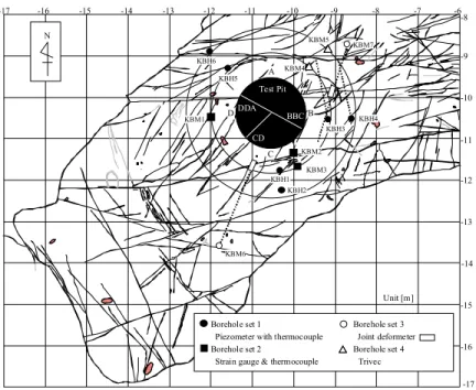
A plan view of the floor of the T-H-M experimental drift in the vicinity of the test hole is shown in Fig. 1.3. A coordinate system has been defined, with the x axis corresponding to the East direction, y axis to the North, and z to the upward vertical direction. The floor is set at z= -2.357 m and the coordinates of the centre of the test hole, at the floor
elevation, is (-10.571,-10.356,-2.357). Four sets of monitoring boreholes were drilled in the rock mass prior to the excavation of the test hole. Set 1 (KBH1 to KBH6) is used to monitor the pore pressure and temperature in the rock mass; Set 2 (KBM1 to KBM3) is used to monitor strain and temperature in the rock mass; Set 3 (KBM4 and KBM5) is used to monitor deformation of the rock mass; and Set 4 (KBM6 and KBM7) is used to monitor the displacements in the main fractures near and intersecting the test pit.
A granulated bentonite was compacted directly into the borehole, by layers of 10 cm in thickness. The initial water content (by weight) of the bentonite was 15%. A heater was installed in the test pit, within the bentonite. When bentonite was compacted within the last 50 cm of the pit, a concrete lid was installed in the remaining part; this lid was restrained by vertical steel bars connected to the ceiling of the drift, in order to restrict vertical movements. A dam was then built on the floor, and a water pool of 40 cm was created. The temperature of the water pool was maintained at 12.3 oC during the duration of the experiment. The heating phase of the experiment started when the temperature at the centre of the heater was set to 100oC; this heating phase lasted 258 days. The heater was then turned off, and the cooling phase started; measurements from the sensors were recorded during a period of approximately 180 days.
Sensors to measure water content, temperature, pore pressure, stress and strain in the bentonite were installed at 3 sections DDA, BBC and CD (Fig. 1.3).
1.3.2 Properties of the buffer
The basic T-H-M properties of the buffer material are determined by laboratory tests. These properties include: saturated permeability, thermal conductivity, Young’s modulus, water retention curves, isothermal infiltration tests, swelling pressure, moisture flow under thermal gradient tests. The details of the tests and the results are given in a separate report. Typical properties are shown in Fig. 1.4 for illustration purposes.
1.3.3 Rock matrix properties
The basic properties of the rock matrix were determined from laboratory tests on intact samples and will be provided in a separate report. Typical values are:
-6 -7 -8 -9 -10 -11 -12 -13 -14 -15 -16 -8 -9 -10 -11 -12 -13 -14 -15 -16 -17 -17 N KBH1 KBH2 KBH3 KBH4 KBH5 KBH6 KBM1 KBM2 KBM3 KBM4 KBM5 KBM6 KBM7 A B C D Test Pit DDA CD BBC
Borehole set 1 Borehole set 3 Piezometer with thermocouple Joint deformeter Borehole set 2 Borehole set 4 Strain gauge & thermocouple Trivec
Unit [m]
Figure 1.3: Mapped fractures on the floor of the test pit and monitoring boreholes.
Density: 2746 (kg/m ); 3
Effective porosity: 0.379 (%); Young’s modulus: 61 (GPa); Poisson’s ratio: 0.303;
Coefficient of linear thermal expansion: 8.21x 10⁻⁶ (oC);
Thermal conductivity:2.54 to 2.71 (W/mo K) (depends on temperature); Specific heat: 900 (J/kgo K);
hydraulic conductivity: 6.6 x10⁻¹⁴ to 1x10-13 (m/s); uniaxial compressive strength: 123 (MPa);
Tensile strength: 11 (MPa).
1.3.4 Properties of the heater
The basic properties of the steel overpack are given below: Density: 7800 (kg/m ); 3
Young’s modulus: 200 (GPa); Poisson’s ratio: 0.3;
Thermal conductivity: 53 (W/mo K); Specific heat: 0.46 (kJ/kgo K);
0 5 10 15 20 25 0.4 0.6 0.8 1 1.2 1.4 1.6 1.8 w (%) th er m al c on duc tiv ity ( W /m/o C ) c) Thermal conductivity 0 5 10 15 20 25 0 100 200 300 400 w (%) E ( M Pa ) b) Young's modulus
1.3.5 Fracture properties and distribution
Mechanical properties of individual fractures were determined by laboratory tests,on sample of 50 to 95 mm in length.The results, including JRC and JCS, shear strength, shear stiffness are available in a separate report. Typical average values are JRC=8.83; And JCS=105 (MPa).
Detailed mapping of the fractures on the floor and roof of the experimental drift, and on the walls of the test hole is also available, together with the in-situ hydraulic test results in the fractured rock mass. Figure 1.3 also shows the most important fractures on the floor of the experimental area.
1.3.6 Output specifications
The time evolution curves for temperature, displacements, water content, etc. in the buffer and the rock mass at specified monitoring points are requested from each team. The details of the locations of the points with monitoring variables can be seen in Jing et al. (1999). The research teams are required to calibrate their computer codes and
computational model with the experimental data. In addition to giving results at the specified points, the results should be evaluated by discussing the following points: • Specify which input parameters are needed in your model. Determine which ones
are available from laboratory and/or field tests, and which ones were assumed, and justify the values actually used in the calibrated model.
• Discuss and justify how the rock-bentonite and bentonite-heater interface was represented
• Discuss how the site of the calibration exercise is applicable to the generic site to be studied in the second phase of BMT1 (e.g. Are the rock mass properties, the degree of fracturing of the rock mass, the bentonite properties, etc. within the range of properties assumed for the generic site?)
1.4 Scoping calculations for the near-field of a generic
repository
1.4.1 Model geometry with different fracture systems for scoping
calculations
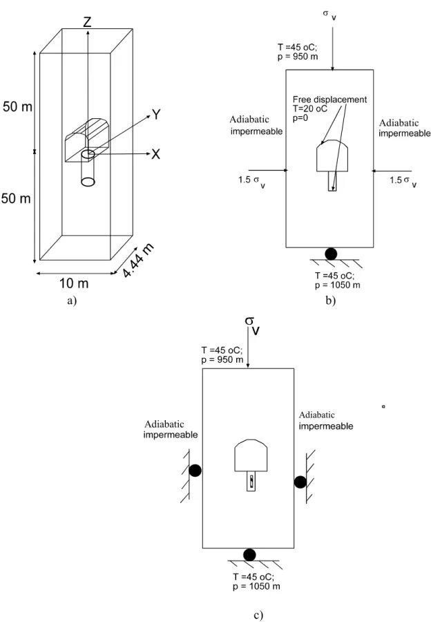
From the conceptual design of the repository (cf. Fig. 1.2), and assuming periodic symmetry, one web of the system, comprising one borehole, and a slice of rock and backfill, is considered. The properties of the rock matrix and overpack are the same as in the calibration exercise. The buffer is a mixture of sand and bentonite; its properties and
the properties of the backfill will be given in separate reports. The model geometry and dimensions are shown in Fig. 1.5a.
The effects of excavation shall be determined by performing a steady-state analysis, with the boundary conditions as illustrated in Figure 1.5b. The output of this analysis consists of contours of temperature, pore pressure, permeability, and factor of safety for rock mass failure at sections x=0 and y=0.
A transient analysis shall be performed, assuming that the buffer, backfill and heater are emplaced instantaneously at time t = 0. The analysis shall be for a period of 200 years. The results from the steady state analysis for excavation effects for temperature, stresses, and pore pressure in the rock mass shall be used as initial conditions. For the buffer and backfill, the initial stresses are assumed to be zero, the initial temperature is 20 oC, and the initial water content is 15 %. The boundary conditions for the transient
analysis are shown in Fig. 1.5c.
Parametric studies considering several degree of fracturing of the rock mass are defined by the following scoping fracture models:
No fracture (Fig. 1.6a) – the BMT1B studies;
One horizontal fracture in the midplane of the emplacement borehole and one vertical fracture 5 m from the tunnel (Fig. 1.6b)- the BMt1C studies;
Two sets of regular fractures of spacing of 0.5m (Fig. 1.6c)-optional BMT1C studies.
For BMT1B studies, the following initial rock mass effective permeability will be considered: 10-19, 10-18, 10-17 m2. The rock mass permeability is assumed to be a function of the effective porosity. This function is derived from experimental data on sparsely fractured rock, with a permeability range of 10-19 to 10-17 m2. The permeability function is shown in Fig. 1.7.
For BMT1C studies, the generation of the fracture will start at position (0,0,0). Each fracture will have the following properties: JRC= 9; JCS = 105 MPa, at a laboratory sample length of 80 mm; initial hydraulic aperture: 10 µm. The rock matrix will have the properties for intact rock defined in section 1.3.3.
The heat output from the waste is shown in Figure 1.8 and given in also tabular form in Appendix 1.
1.4.2 Output specifications for buffer and backfill
Time histories of temperature, water content and stresses in the buffer at the output points shown in Fig. 1.9 and Table 1.1 will be calculated. The time history of the vertical displacement at B1 shall also be calculated.
The contours of temperature and water content in the buffer and backfill, at sections x=0 and y=0 shall be plotted at times: 1, 2, 4, 8, 16, 32, 64, 128, and 200 years.
Adiabatic Adiabatic a) b) Adiabatic Adiabatic c)
Figure 1.5: Geometry model for near-field scoping calculations a) and boundary conditions for the excavation effect simulation b) and transient analyses c).
Fractures Intact Rock Homogeneous
Intact Rock Back-fill
Canister Bentonite
Figure 1.6: Geometry of alternative fracture models.
0 1E-007 2E-007 3E-007
n**3 0 2E-017 4E-017 6E-017 k ( m **2 ) k (m2) = 2.186× 10⁻¹⁰n3– 5.8155.× 10–18 r2= 0.909 1 100 10000 1000000 100000000 1.000E+10 0 100 200 300 400 Time (yr) H eat ou tp ut ( W ) a) b) c) Figure 1.7: Permeability as a function of effective porosity
Figure 1.8: Heat output from the waste
Figure 1.9: Output points for buffer
1.4.3 Output specifications for rock mass
Contours at sections: x=0 and y=0 and variations along monitoring lines: x=y=0; z=-0.41 & x=0; z=-z=-0.41 & y=0 will be plotted at times 1, 2, 4, 8, 16, 32, 64, 128, and 200 years for the following output parameters: i) temperature and pore pressure; ii) Factor of safety for rock mass failure; and iii) Permeability.
1.4.4 Evaluation of coupling effects
For both the excavation phase, and the long term phase with emplaced buffer, backfill and heater, the analyses shall be performed with increasing degree of complexity of coupling. A comparison matrix will be established in order to compare the implications of various orders of complexity of the coupling, as shown in Table 1.2.
1.4.5 Rock mass failure criterion
The Hoek-Brown failure criterion is adopted to estimate the rock mass strength behaviour for BMT1, and is expressed in effective stress as
2 ' 3 ' 3 ' 1 σ mσcσ sσc σ = + + (1.1)
Table 1.1: Output points for buffer
Point x (m) y (m) z (m) Output values
B1 0 0 0 T, θ, σzz , uz B2 0 0 -0.85 T, θ, σxx, σzz B3 0 0 -1.7 T, θ, σxx, σzz B4 0.41 0 -2.665 T, θ, σxx B5 0.76 0 -2.655 T, θ, σxx, σzz B6 1.11 0 -2.655 T, θ, σxx B7 0 0 -3.43 T, θ, σzz B8 0 0 -3.78 T, θ, σxx, σzz B9 0 0 -4.13 T, θ, σzz B10 0.76 0 -0.85 T, θ, σxx, σzz B11 0.76 0 -3.78 T, θ, σxx, σzz B12 0 0.41 -2.665 T, θ, σyy B13 0 0.76 -2.655 T, θ, σxx, σzz B14 0 1.11 -2.655 T, θ, σyy B15 0 0.76 -0.85 T, θ, σxx, σzz B16 0 0.76 -3.78 T, θ, σxx, σzz
Table 1.2: Comparison matrix of for different degree of THM coupling
Output
T M H H-M T-H T-M T-H-M
T-evolution Y N/A N/A N/A Y Y Y
σ-evolution N/A Y N/A Y N/A Y Y
k-evolution N/A N/A N/A Y Y N/A Y
p-evolution N/A N/A Y Y Y N/A Y
θ-evolution N/A Y Y Y Y N/A Y
where ' 1
σ and '
3
σ are the major and minor effective principal stresses at failure when
equation (1.1) is satisfied, and the effective stress components are defined through ij
ij ij σ pδ
σ' = − (1.2)
The symbol σcis the uniaxial compressive strength of the rock (=123 MPa), and
parameters m and s are the empirical constants, with m=17.5 and s = 0.19, respectively.
1.4.6 Interfaces between buffer/rock mass, backfill/rock mass and
overpack/buffer
It is difficult to provide standard models for the interfaces between buffer and rock, between backfill and rock and between overpack(heater) and rock, mainly due to lack of existing models and available supporting data. The research teams shall therefore define their own assumptions for the nature of these interfaces, from the experience gained in the calibration of the T-H-M test previously discussed.
1.4.7 Uncertainty evaluation
Since the buffer and backfill are man-made materials, it is assumed in this exercise that their properties could be considered constant. The most important degree of
uncertainty would be related to the characteristics of the rock mass, e.g. the matrix permeability, the rock mass equivalent permeability, the fracture density and possibly orientation. It is hoped that the consideration of different cases in this exercise (BMT1B and BMT1C) would serve to span a wide span of rock mass characteristics. For example, F0 would constitute a case where no distinctive fracture need to be explicitly included, and the rock mass could be considered as an equivalent porous medium with a range of
permeability from 10-19 to10-17 m2. F1 would constitute a scenario where one important
fracture crosses the borehole, and F2 and F3 would constitute the scenario with
ubiquitous fractures. The last task of this BMT1 would be a synthesis of all output results from F1 to F4, where the RTs should compare safety features (i.e. temperature field, time for resaturation, stress field, permeability change, potential for rock mass failure)
between cases F0 to F5. The other source of uncertainty might be the way the interfaces between the buffer/rock mass, backfill/rockmass and overpack/buffer are considered in the model. The RTs should discuss the influence of these interfaces on their results.
1.5 A Simplified axisymmetric calibration case of the
T-H-M in-situ experiment at Kamaishi Mine – case
definition of BMT1A
Previous experiences with Task 2 in DECOVALEX II shows that the physics in BMT1 is quite complex and a simple calibration test case with a much simplified problem
geometry, but including all relevant physical processes might be helpful to understand the interactions between physical processes, especially the effects of mechanical
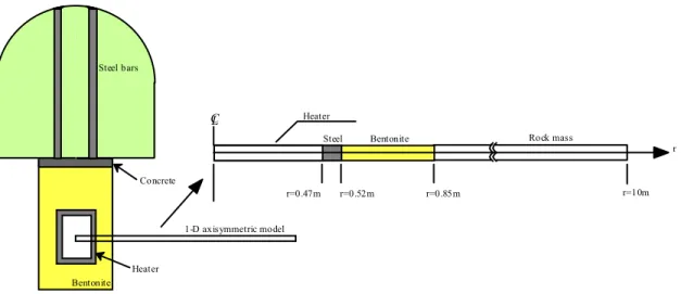
deformation. For this purpose, a simplified calibration test case was proposed and defined below. The case focuses on the THM behaviour of one radial line from the centre of the heater, with the axisymmetric geometry shown in Fig. 1.10.
The desired output at 5 points, shown in the figure is detailed in Table 1.3. Time histories of these output parameters are requested for a heating period of 258 days followed by a cooling period of 180 days.
1-D axisymmetric model Steel bars Concrete Heater Bentonite Heater
Bentonite Rock mass
r=0.52m r=0.85m r=10m CL
r r=0.47m
Steel
Figure 1.10: Geometry of the simplified axisymmetric model.
Table 1.3: Output variables and locations for the simplified axisymmetric model
Point r (m) Output 1 0.52 T, u, σ,εr, w 2 0.685 T, u, σ,εr, w 3 0.85 T, u, σ,εr, w 4 1.45 T,u, p, εr , εt 5 3. T,u,p
The units of the variables are: T- temperature (°C), u- radial displacement (m), p- pore
pressure (Pa), w- water content by weight (%), σ− radial total stress (Pa) and εr , ε
radial and tangential strain (non-dimensional). The boundary conditions are as follows: At r = 0.47 m:
T=100 oC (during heating) and free temperature (during cooling)
Free displacement
Impermeable
At r = 10 m:
T = 12 oC
u=0
p=3.9 kPa (equivalent to 0.4 m of water)
The initial conditions are as follows:
T = 12 oC everywhere
The displacements and stresses are zero everywhere
p =3.9 kPa in the rock; w =15% in the bentonite
The basic T-H-M properties of the bentonite are determined by laboratory tests by JNC (1997). Depending on the models, input properties additional to the ones determined in the laboratory might be needed. These additional properties were determined by
performing calibration of laboratory tests performed in Task 2C, of DECOVALEX II (Jing et al., 1999). For this test case, the input properties should be selected from these two sources, especially the Table 5.1 in Jing et al. (1999), which summarizes the most important input parameters and should be used as a starting point.
The following experimental values should be used as calibration targets: temperature and water content at points 1, 2 and 3; radial stresses at points 1and 3; radial strain at point 2 and radial and tangential strain at point 4. These experimental data came from the recorded results of different sensors at the same radial distance, but at different tangential angles. In addition, tensile stress measurements may or may not be reliable and cafre should be taken in using them.
This report presents the works performed for BMT1-A. The authors of the chapters are: T. S. Nguyen (Chapter 2), M. Chijimatsu and Y. Sugita (Chapter 3), J. Rutqvist (Chapter 4), A. Thoraval, M. Souley and A. Giraud (Chapter 5), A. Millard and A. Rejeb (Chapter 6), T. S. Nguyen and L. Jing (Chapters 1 and 7).
17
2. Re-evaluation of the Kamaishi mine
modelling- The CNSC team studies
In this chapter, the works performed by the CNSC (formerly AECB) team on the first phase of BMT1 is presented. The objective of this first phase is to increase the
confidence in the modelling tool, the FRACON finite element code. The FRACON code will be also be used for scoping calculations latter phases of BMT1, looking at safety issues related to THM processes in the near-field. The strategy to increase this confidence is to obtain a better understanding of the physical processes that actually prevailed during the in-situ THM experiment performed a the Kamaishi mine in Japan. Blind prediction of the experiment was performed by the CNSC team (Nguyen, 1999; Nguyen, 2000 a and b) during DECOVALEX II. The chapter will first summarize the results of the former work, pointing out the agreement, or lack of it, between predictions and experimental results; discuss possible explanations for the disagreements; and finally present the results of a new analysis in an attempt to reconcile the differences.
2.1 Summary of blind prediction of the Kamaishi THM experiment
As part of DECOVALEX II project, the FRACON code was used to perform blind predictions of the experiment. An axisymmetric model was used in DECOVALEX II (Fig. 2.1). The degree of agreement between the predictions and the experimental results could be summarized as follows:
Temperatures are very well predicted in both the bentonite and the rock mass (Fig. 2.2)
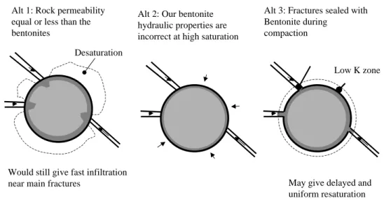
The water content in the bentonite are well predicted (Fig. 2.3). At the rock/bentonite interface, the model predicts a faster resaturation than the experimental data. It was believed that this is due swelling of the bentonite that in turns creates a sealing effect at the interface.
The total stresses in the bentonite are well predicted at the rock/bentonite interface; these stresses were overpredicted near the heater (Fig. 2.4). It was believed then that this overprediction is due to the assumption of an infinitely rigid heater.
The displacements in the rock were reasonably well predicted (Fig. 2.5).
The pore pressure in the rock mass, induced by the thermal pulse, was predicted to be insignificant. The experimental data did show some small effects. It was believed that this is due to the coarseness of the mesh used in the finite element model.
2.2 The simplified axi-symmetric model
In order to test the adequacy of the hypotheses formulated in section 2.1, with respect to the lack of agreement between predicted and experimental results, a re-evaluated
18
pressure = 0.4 m water free displacement T =12 oC
impermeable zero normal displacement T =12 oC impermeable; zero normal displacement; T =95 oC hydrostatic; zero normal displacement; T =12 oC 0 100 200 300 400 500 Time (day) 5 10 15 20 25 30 T ( o C ) RT1 RT2 RT3 0 100 200 300 400 500 Time (day) 0 20 40 60 80 T ( o C ) BT4 BT1
a) temperature in bentonite b) temperature in rock
Figure 2.2: Temperature evolution (dots are predicted values) - DECOVALEX II
0 100 200 300 400 500 Time (day) 0 5 10 15 20 25 G rav im e tr ic wat e r c ont ent ( % ) BW1 measured (WE32) Measured (WE36) FRACON 0 100 200 300 400 500 Time (day) 0 5 10 15 20 25 G rav im e tr ic wat e r c o n tent ( % ) BW5 Measured (HM5H) Measured (HM7H) FRACON
a) Water content near heater b) water content at bentonite/rock interface
Figure 2.3: Water content evolution (dots are predicted values) - DECOVALEX II Figure 2.1: CNSC (formerly
AECB) finite element model for prediction of Kamaishi Mine THM experiment in DECOVALEX II
19 0 100 200 300 400 500 Time (day) -2000000 0 2000000 4000000 6000000 8000000 T o ta l s tre ss (P a ) BP5 FRACON Measured (PS15) 0 100 200 300 400 500 Time (day) -1600000 -1200000 -800000 -400000 0 400000 T o ta l st re ss (P a ) BP4 FRACON Measured (PS12)
a) stresses at buffer/rock interface b) stresses near heater
Figure 2.4: Evolution of total stress in bentonite - DECOVALEX II
0 100 200 300 400 500 Time (day) -0.0002 0 0.0002 0.0004 0.0006 V e rt ic al di sp lac e m ent ( m ) RD1 (predicted) RD1 (measured) RD3 (predicted) RD3 (measured)
conceptual model was formulated y the CNSC team, as the simplified axisymmetric model defined in Chapter 1. The attention is focussed on one line of radial symmetry running through the centre of the heater (cf. Fig. 1.11); consequently a thin layer of material running through this line is considered in the finite element model (Fig. 2.6). The finite element model is actually a quarter of a thin cylinder. Using symmetry arguments, the bottom, top, x=0 and y=0 boundaries are assumed to be adiabatic, impermeable and with zero normal displacements. A constant temperature of 100 oC was imposed on the left boundary, as dictated by the set temperature in the centre of the heater, during the heating phase of 258 days. The above thermal constraints was
released during the subsequent cooling period of 180 days. A constant water pressure of 3.9 KPa (corresponding to a height of 0.4 m of water imposed on the floor of the
experimental drift) was imposed on the right boundary, situated at a radial distance of 3 m. Zero normal displacement was also imposed at the right boundary. The whole system
Figure 2.5: Displacement in rock mass - DECOVALEX II
20 Rock mass Bentonite Heater -100 0 100 200 300 400 500 Time (day) 0 40 80 120 T ( o C ) Pt 3 Pt 2 Pt1 Pt 3 (exp) Pt 2 (exp) Pt 1(exp)
was initially set at a temperature of 12 oC. In order to match the measured temperature, it was assumed that all nodes from a radial distance of 2.27 m to 3 m remained at a constant temperature of 12 oC.
The input properties of the bentonite and the rock mass remains the same, except for the following:
A “stiffer” bentonite with a Young’s modulus of 150 MPa as compared to 50 MPa. Near the heater, within an annulus of 4 cm in thickness, the Poisson’s ratio was also increased from 0.4 to 0.484. This adjustment was necessary in order to decrease the predicted value of the stresses to levels consistent with the
measured values.
The heater was included in the model, with the following input properties: Young’s modulus 200 GPa and Poisson’s ratio: 0.4.
The results for temperature in the bentonite are shown in Fig. 2.7. Except for some numerical dispersion in the calculated values (existence of an artificial peak temperature during the heating phase), very good agreement is obtained between calculated and measured temperatures.
The water content evolution in the bentonite is shown in Fig. 2.8. Good agreement is
Figure 2.6:Finite element for the simplified
axisymmetric model
Figure 2.7: Temperature in bentonite.
21
obtained near the heater. Reasonably good agreement is obtained at the rock/bentonite interface. The resaturation predicted by FRACON occurs much faster (4 days) than indicated by the measured data (100 days), even with the introduction of a thin layer of rock (2 cm), with permeability values which are intermediate between the bentonite and the remaining rock mass. It is possible that the rock was initially unsaturated. The calculated water content does not compare well with the measured values for point 2; this might be due to the inability of the FRACON code to take into account
condensation/evaporation processes.
The total radial stress at point 1, near the heater, is shown in Fig. 2.9. Good
agreement is also obtained between calculated and measured results. Stresses are shown to be mostly compressive (positive values).
The evolution of total radial stress at point 3, at the bentonite/rock interface is shown in Fig. 2.10. Reasonably good agreement is obtained; the stresses seem to be mostly tensile (negative values). At cooling, the calculated stress shows a reversal in the variation trends while this was not evident from the experimental results.
0 100 200 300 400 500 Time (day) 0 5 10 15 20 25 W ( % ) Pt 3 Pt 2 Pt 3 Pt 2 (exp) Pt 1 (exp) Pt 3 (exp) 0 100 200 300 400 500 Time (day) -400000 0 400000 800000 1200000 T o ta l st re ss ( P a ) PS15 - exp PT 1 - FRACON PS 11 - exp PS13 - exp Figure 2.8: Evolution of water content in bentonite Figure 2.9: Total radial stress at point 1, near heater
22
The evolution of radial strain at point 2 in the bentonite, midway between the heater and the rock, is shown in Fig. 2.11. Tensile straina (negative values) are predicted. The predicted values agree well with the measured ones, if a sign reversal is brought to the latter (according to JNC, the measured strain are compressive). The calculated radial displacements at points 1, 2 and 3 in the bentonite are shown in Fig. 2.12, where positive values denote outward movements. Points 1 and 3 are predicted to move
outward due to thermal expansion, while point 2 would move inward, due to swelling of the bentonite caused by wetting (increase in water content).
The temperature, radial displacement, pore pressure, and strain at point 4 in the rock are shown in Figs. 2.13 - 2.16, respectively. In Fig. 2.15, a thermally induced pressure pulse is predicted by the FRACON code. This pulse is of very short duration, since the rock is relatively permeable. The axial strain are calculated to be tensile and follows the same trends as the measured strain; however the calculated axial strain is about one order of magnitude lower than the measured strain. The calculated tangential strain, contrarily to the measured strain, is also tensile. These discrepancies are likely due to the prescribed fixed boundary condition at a radius of 3 m; the right boundary of the finite element model (cf. Fig. 2.6) should be extended to farther distances.
0 100 200 300 400 500 Time (day) -1600000 -1200000 -800000 -400000 0 400000 800000 T o ta l s tre ss (P a ) BP4 Measured (PS12) Pt 3 - FRACON Measured (PS-12) -100 0 100 200 300 400 500 Time (day) -0.016 -0.012 -0.008 -0.004 0 0.004 0.008 Ra d ia l s tr a in KM7-exp KM8-exp FRACON Figure 2.10: Evolution of total radial stress at point 3 (bentonite/ro ck interface) Figure 2.11: Evolution of radial strain in buffer at point 2 (midway between heater and rock)
23 0 100 200 300 400 500 Time (day) -0.003 -0.002 -0.001 0 0.001 Ra d ial dis p la ce m e n t ( m ) Point 1 Point 2 Point 3 0 100 200 300 400 500 Time (day) 10 15 20 25 30 35 T e m p er a tur e ( o C ) 0 100 200 300 400 500 Time (day) -5E-005 0 5E-005 0.0001 0.00015 0.0002 0.00025 Ra dial dis p lac e m ent ( m ) Figure 2.12: Radial displacement in bentonite. Figure 2.13: Calculated temperature at point 4 in rock mass Figure 2.14: Calculated radial displacement in rock mass
24 0.001 0.01 0.1 1 10 100 1000 Time (day) -200000 0 200000 400000 600000 800000 1000000 P o re P re ss u re (P a ) -100 0 100200300400500 Time (day) -0.002 -0.001 0 0.001 Str a in epsr - FRACON epst - FRACON epsr - experimental epst - experimental
2.3 Summary and conclusion
The results from the “one-dimensional” axisymmetric model used in the re-evaluation of the Kamaishi mine experiment showed general improvement over the “2-dimensional “ axisymmetric model used in the prediction phase:
As before, calculated values of temperature agree very well with the experimental values
By defining a “stiffer” bentonite, the calculated stress and strain in the bentonite agree well with the experimental values.
The water content near the heater are well predicted. The saturation front at the bentonite/rock interface are still predicted to advance much faster than in reality, even with the use of a low permeability rock layer at this interface. It is possible that an unsaturated rock layer exists around the bentonite. The calculated water content in the bentonite does not agree well with the experimental data and the FRACON code needs to be modified to include condensation and evaporation. The strain in the rock is underpredicted; this is probably due to the fixed
boundary condition imposed at too short a radial distance (3 m) from the centre of the heater. Figure 2.15: Calculated pore pressure at point 4 in rock mass Figure 2.16 Strain at point 4 in rock mass
3. Re-evaluation of Kamaishi mine modeling-
The JNC/KIPH team studies
3.1 Introduction
This section presents the work conducted by the JNC/KIPH Research team on the first phase of BMT1. The objective is to re-evaluate the modeling of the Kamaishi Mine heater test (Chijimatsu et al., 1999). In order to carry out the re-evaluation, the modeling of swelling pressure buffer material considering both the temperature and the density dependencies based on the laboratory experiment results, carried out by Japan Nuclear Cycle Development Institute, is performed at first. Then validation of this model was conducted by using the laboratory test and re-evaluation of Kamaishi heater test was carried out by an simplified axisymmetric model.
3.2 Temperature and density dependency of swelling
pressure
3.2.1 Temperature dependency
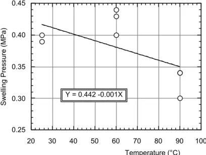
Figure 3.1 shows the swelling pressure measurement results (Suzuki and Fujita, 1999). Material of the specimen was sand mixture bentonite (B:S=7:3, Dry density is 1.6 g/cm3). During the swelling pressure measurement, temperature increased step by step as shown Figure 3.1. Table 3.1 shows the final swelling pressure value of each temperature condition. Figure 3.2 shows the relationship between final swelling pressure value and temperature. In these figures, swelling pressure at 60ºC is higher than that at 25ºC in this experiment. However it is assumed that swelling pressure decreases with increases in temperature linearly as shown Figure 3.2 because swelling pressure at 90ºC is lower than that at 25ºC. The function of swelling pressure σ and temperature T is given by.
σ = 0.44 - 0.001T (3.1)
From this equation, the swelling pressure at 25ºC is calculated to be 0.415 MPa.
3.2.2 Density dependency
Figure 3.3 shows the relationship between the swelling pressure and the effective density of the buffer. This relationship is expressed by equation (3.2) (Japan Nuclear Cycle Development Institute, 2000), using the effective density calculated by equation (3.3). From equation (3.2), in the case of sand mixture bentonite (B:S=7:3) at a dry density of 1.6g/cm3, the effective density is 1.368g/cm3 and the swelling pressure was calculated to be 0.48 MPa. The density of the soil particles is assumed to be 2.65g/cm3.
26
σ = exp(3.85ρe2-7.33ρe+2.09) (3.2)
ρe = ρd(100-Rs)/(100-ρd Rs/ρs) (3.3)
where, ρe is effective density (g/cm3), ρd is dry density (g/cm3), Rs is mixing ratio at dry
weight of sand (%) and ρs is the density of the soil particles (g/cm3), respectively.
0.0 0.1 0.2 0.3 0.4 0.5 20 30 40 50 60 70 80 90 100 0 1000 2000 3000 4000
Swelling pressure [MPa]
Temperature [°C]
Time [hour]
Temperature Swelling pressure
Figure 3.1: Measurement results of swelling pressure with time
0.25 0.30 0.35 0.40 0.45 20 30 40 50 60 70 80 90 100
Swelling Pressure (MPa)
Temperature (°C) Y = 0.442 -0.001X
Figure 3.2: Relationship between swelling pressure and temperature Table 3.1: Measurement results of swelling pressure (MPa)
Temperature 25ºC 60ºC 90ºC Swelling pressure 0.39 0.40 0.40 0.43 0.40 0.44 0.34 0.30 0.34
10-1
100
101
102
1.0 1.2 1.4 1.6 1.8 2.0 2.2
Swelling pressure (MPa)
Effective clay density (g cm-3)
σ=exp(3.8497ρ e 2 -7.3332ρ e+2.0856) (1.2≦ρ e≦2.0)
Figure 3.3: Relationship between effective clay density and swelling pressure
3.2.3 Modeling of swelling pressure
From the above results, it is assumed that swelling pressure is a function of temperature and effective density as shown in equation (3.4). In the THM simulation, the swelling pressure is modeled as a function of water potential as shown in equation (3.5), in which the coefficient F is estimated by back analysis of laboratory test. Therefore, the estimated coefficient value from the swelling pressure at temperature 25ºC, dry density 1.6 g/cm3, sand mixing ratio 30% is to be Fo and the THM simulation
is conducted by using F value shown in equation (3.6).
σ=exp(3.85ρe2-7.33ρe+2.09)-0.001T (3.4) σ=F∆ψ (3.5)
(
)
(
)
⎪⎭ ⎪ ⎬ ⎫ ⎪⎩ ⎪ ⎨ ⎧ − + − − + − × = o eo eo e e o T T F F 001 . 0 09 . 2 33 . 7 85 . 3 exp 001 . 0 09 . 2 33 . 7 85 . 3 exp 2 2 ρ ρ ρ ρ (3.6) where To =25ºC and ρeo =1.368g/cm33.3 Simulation of laboratory experiment by
considering temperature and density dependencies
3.3.1 Simulation of swelling pressure tests
The simulation of swelling pressure tests at each temperature was conducted and compared with measurement results. The simulation was carried out with an axisymmetric model as shown in Figure 3.4. The material is sand mixture bentonite with dry density 1.6 g/cm3. Temperature is 25ºC, 60ºC and 90ºC. Figures 3.5 and 3.6
28 20mm 10mm C L No Flux No Flux P=0
show the water diffusivity and water retention curves, respectively. For the simulation, the experimental function (3.7) is adopted for water diffusivity and the van Genuchten model (3.8) is adopted for water retention curve. Table 3.2 shows the coefficients for equations (3.7) and (3.8). Table 3.3 shows the other parameters of sand mixture bentonite. 10-7 10-6 10-5 10-4 10-3 0 0.05 0.1 0.15 0.2 0.25 0.3 0.35 0.4 0.45 Measured (25°C) Measured (40°C) Measured (60°C) Function (25°C) Function (40°C) Function (60°C) Water diffusivity [cm 2 /s]
Volumetric water content [cm3/cm3]
102 103 104 105 106 107 108 0 0.05 0.1 0.15 0.2 0.25 0.3 0.35 0.4 0.45 Measured (25°C) Measured (40°C) Measured (60°C) van Genuchten model
Water potential head [cm]
Volumetric water content [cm3/cm3]
Figure 3.4: Analysis model for swelling pressure test
Figure 3.5: Water
diffusivity of sand mixture bentonite
Figure 3.6: Water retention curve of sand mixture bentonite
(
)
(
)(
)
2(
2)
2 1 1 1 b b a b b a D s s − + − − − = θ θ θ θ θ θ θ (3.7){
}
⎟ ⎠ ⎞ ⎜ ⎝ ⎛ − − + = − − n n r s r 1 1 1 αψ θ θ θ θ (3.8) Table 3.2: Coefficients for equations (3.7) and (3.8)Coefficient Value a1 2.99·10-8T - 3.74·10-7 a2 -1.50·10-8T + 1.49·10-7 b1 - 2.49·10-3 b2 5.59·10-4T + 3.93·10-1 θs 0.403 θr 0.000 α 8.0·10-5 n 1.6
Table 3.3: Other parameters
Parameter Value
Young’s modulus (MPa) 50.0
Poisson’s ratio 0.3
Intrinsic permeability (m2) 4.0·10-20 Thermal conductivity (W/m/K) 4.44·10-1+1.38·10-2ω
+6.14·10-3ω2-1.69·10-4ω3 Specific heat (kJ/kg/K) (34.1+4.18ω)/(100+ω) Thermal expansion coefficient (1/K) 1.0·10-5
Thermal water diffusivity (m2/s/K) 7.0·10-12
Figure 3.7 shows the time history of the water potential in each section in the specimen. The legend in the figure shows the distance from the bottom of specimen, i.e. the distance from the seepage surface. Figure 3.8 shows the time history of water content in each section, which is higher close to the seepage surface. The specimen became saturated after approximately 300 hours. Figure 3.9 shows the time history of total pressure at each section. Because of the swelling pressure generated by the change of water potential, as used in the model, the tendency of swelling pressure generation is similar with the water potential change. Furthermore, swelling pressure became constant when the change of water potential was stopped. The swelling pressure value at the seepage side was lower than that at the opposite side, but the difference is small. Figure 3.10 shows the time history of strain at each section in the specimen. Positive values show compressive strain and negative values show tensile strain. Tensile strain occurred near the seepage surface and compressive strain occurred at the opposite side. Both tensile and compressive strains decreased with saturation of the specimen, and became zero when the specimen was fully saturated. Figure 3.11 shows the time history of dry density at each section of the specimen, which decreased at the bottom side due to the generation of the tensile strain at the early time. At the upper side it increased. The change of dry density disappeared when swelling pressure became constant, and afterwards the dry density in the specimen became uniform. Figure 3.12 shows the comparison of swelling pressures between calculated and measured results. Experiments were carried out five times and the results show the different swelling
pressure values. The coefficient Fo was estimated to simulate the average swelling
30 -140000 -120000 -100000 -80000 -60000 -40000 -20000 0 0 100 200 300 400 500 0.10cm 0.50cm 1.00cm 1.50cm 2.00cm Time(hour) W
ater potential head (cm)
Figure 3.7: Time history of water potential in each section (Temperature is 25ºC)
0 5 10 15 20 25 30 0 100 200 300 400 500 0.05cm 0.55cm 1.05cm 1.55cm 1.95cm Time [hour] W ater Content [%]
Figure 3.8: Time history of water content in each section (Temperature is 25ºC)
0.00 0.10 0.20 0.30 0.40 0.50 0 100 200 300 400 500 0.05cm 0.55cm 1.05cm 1.55cm 1.95cm Time(hour)
Total pressure (MPa)
-6.0 10-3 -4.0 10-3 -2.0 10-3 0.0 100 2.0 10-3 4.0 10-3 0 100 200 300 400 500 0.15cm 0.55cm 1.05cm 1.55cm 1.95cm Time(hour) Strain
Figure 3.10: Time history of strain in each section (Temperature is 25ºC)
1.57 1.58 1.59 1.60 1.61 1.62 0 100 200 300 400 500 0.05cm 0.35cm 0.65cm 1.05cm 1.35cm 1.65cm 1.95cm Time(hour) Dry density ( g/cm 3 )
Figure 3.11: Time history of dry density in each section (Temperature is 25ºC)
0.0 0.1 0.2 0.3 0.4 0.5 0.6 0 300 600 900 1200 1500 1800 Measured(No.1) Measured(No.2) Measured(No.3) Measured(No.4) Measured(No.5) Estimated Pressure [MPa] Time [hour]
32
Figure 3.13 and Figure 3.14 shows the time history of water content and total pressure at each section in the specimen when the temperature is 60ºC, respectively. Figure 3.15 and Figure 3.16 also show the time history of water content and total pressure at each section in the specimen when the temperature is 90ºC. The time needed for the specimen becoming fully saturated decreases with increasing temperture and the time needed for the swelling pressure becoming constant also decreases. Furthermore, the swelling pressure value decreases with increasing temperature.
3.3.2 Simulation of the coupled test in laboratory
3.3.2.1 Outline of coupled test
Figure 3.17 shows the test apparatus used for the coupling test, which consists of the water movement under a thermal gradient and water injection (Suzuki et al., 1999). The test apparatus is composed of a specimen, a main unit of 50-mm in diameter and 100-mm in height, a heating chamber, a copper plate, a thermostat with a circulation system, thermocouples, load cells, and a data logger. During the test, the temperature of the thermostat connected to the heating chambers above and below the specimen is controlled at specified temperature. Furthermore, water is injected from the upper side of the specimen at water head of 100cm. Measurement items are total infiltration quantity into the specimen, temperature and swelling pressure. Temperature is measured by thermocouple at locations 0.2, 2.0, 4.0, 6.0, 8.0, 9.8cm from the bottom of the specimen, respectively, with the data logger. Swelling pressure is measured by load cell at locations 1.0, 3.0, 5.0, 7.0, 9.0cm from the bottom of the specimen, respectively, with the data logger. Swelling pressure is also measured at the upper surface of the specimen. The water distribution is obtained by measuring the water content by the oven-dry method after dividing the specimen in the apparatus when test is finished.
3.3.2.2 Measurement result
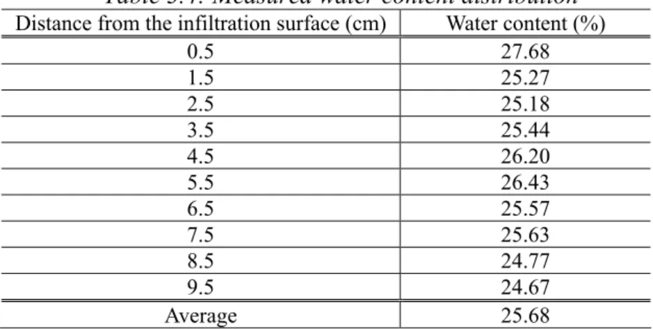
Figure 3.18 shows the time history of infiltration quantity into the specimen. 65cc of water injected into the specimen and injection was stopped after 7000 hours. Theoretical maximum infiltration quantity is approximately 60cc. The reason for less measured infiltration quantity than the theoretical one was considered to be the influence of evaporation of water. Figure 3.19 shows the time history of the swelling pressure. The swelling pressure also becomes constant after 7000 hours and this agrees with the change in infiltration quantity. The value of the swelling pressure is approximately 0.4 MPa at the upper side of specimen and approximately 0.2MPa at the lower side of specimen. That means that the swelling pressure at the upper side is higher than that at the lower side. The upper side is the infiltration side with lower temperature under a thermal gradient. After the coupled test was finished, the water content distribution was measured and Table 3.4 shows the results. The theoretical saturated water content of this specimen is approximately 25% and it is judged that the specimen after coupled test was almost saturated. From Table 3.4, it is shown that the water content at the infiltration side and center part of the specimen is higher than other part.
The reason of the high water content at the infiltration side is due to the swelling at the early stage of coupled test. The reason of high water content at the center part is due to the low dry density of this part due to difficulty of uniform manufacturing.
0 5 10 15 20 25 30 0 100 200 300 400 500 0.05cm 0.55cm 1.05cm 1.55cm 1.95cm Time [hour] W ater Content [%]
Figure 3.13: Time history of water content in each section (Temperature is 60ºC)
0.00 0.10 0.20 0.30 0.40 0.50 0 100 200 300 400 500 0.05cm 0.55cm 1.05cm 1.55cm 1.95cm Time(hour)
Total pressure (MPa)
Figure 3.14: Time history of total pressure in each section (Temperature is 60ºC)
0 5 10 15 20 25 30 0 100 200 300 400 500 0.05cm 0.55cm 1.05cm 1.55cm 1.95cm Time [hour] W ater Content [%]
34 0.00 0.10 0.20 0.30 0.40 0.50 0 100 200 300 400 500 0.05cm 0.55cm 1.05cm 1.55cm 1.95cm Time(hour)
Total pressure (MPa)
Figure 3.16: Time history of total pressure in each section (Temperature is 90ºC)
THERMOSTAT WITH CIRCULATION SYSTEM 30.0 AIR LAYER COPPER PLATE THERMOCOUPLE COMPACTED BENTONITE SPECIMEN 18 18 20 20 20 40.0 10 10 20 20 20 20 LOAD CELL LOAD CELL AIR OUTLET WATER INLET PISTON 10 0 50 unit [mm] (100)
0 10 20 30 40 50 60 70 0 2000 4000 6000 8000 10000 In filt rat ion quant ity [ cc]
Elapsed time [hour]
Figure 3.18: Measured infiltration quantity into the specimen
0 0.1 0.2 0.3 0.4 0.5 0 2000 4000 6000 8000 10000 σ
c(Distance from the bottom 1cm)
(Distance from the bottom 3cm)
(Distance from the bottom 5cm) (Distance from the bottom 7cm)
(Distance from the bottom 9cm) σ
a
Swelling Pres
su
re [MPa]
Elapsed time [hour]
Figure 3.19: Measured swelling pressure
Table 3.4: Measured water content distribution Distance from the infiltration surface (cm) Water content (%)
0.5 27.68 1.5 25.27 2.5 25.18 3.5 25.44 4.5 26.20 5.5 26.43 6.5 25.57 7.5 25.63 8.5 24.77 9.5 24.67 Average 25.68 3.3.2.3 Analysis model
The analysis was carried out with an axisymmetric model (Fig. 3.20). For the thermal boundary conditions, the upper surface was fixed with a temperature of 30ºC and the bottom surface with 39ºC. The side of the model was adiabatic. For the hydraulic
36
boundary conditions, the upper surface was fixed with a water head of 100-cm and other surfaces were no flow boundaries. The initial water content was 6.0%. Mechanically all surfaces were fixed with a zero normal displacement.
3.3.2.4 Analysis results
Figure 3.21 shows the time history of water content in the bentonite. Legend X expresses the distance from the bottom surface of the specimen. That is, X=0 cm is the high temperature surface and X=10 cm is the low temperature surface. It shows that the low temperature side (the infiltration side) became saturated earlier than the opposite side (the higher temperature side). Water content at the high temperature side decreased at first, however the influence of temperature was small and water content increased latter. After 8000 hours from the start, water content change became steady, and at the upper side it was approximately 25%, indicating that the upper side was saturated. The water content at the lower side was smaller than that at the upper side.
Figure 3.22 shows the time history of dry density. It shows that the dry density near the infiltration side became low at the early time of experiment due to swelling. However, the dry density at the high temperature side also became low finally. From this result, it was expected that the saturated water content at the high temperature side should become higher than 25%. However, as a result of the simulation, the water content at the high temperature side became lower than 25%, i.e. not saturated. Figure 3.23 compares the water infiltration quantity between calculated and measured results, with good agreement in general tendency, but different final values. The estimated water infiltration quantity was less than 60cc because the theoretical maximum value of water infiltration quantity was approximately 60cc.
Figure 3.24 shows the time history of total pressure in each section. As a result of simulation, total pressure at the high temperature side was lower than that at the low temperature side and this tendency is similar to the measured result.
100mm 25mm C L No Flux No Flux T=40ºC H=100cm T=30ºC
0 5 10 15 20 25 30 0 2000 4000 6000 8000 10000 X=0.1 X=2.1 X=4.1 X=6.1 X=8.1 X=9.9 Water content [%]
Elapsed time [hour]
Figure 3.21: Time history of water content by simulation
1.585 1.590 1.595 1.600 1.605 1.610 1.615 0 2000 4000 6000 8000 10000 X=0.1 X=2.1 X=4.1 X=6.1 X=8.1 X=9.9 Dry density [g/cm 3 ]
Elapsed time [hour]
Figure 3.22: Time history of dry density by simulation
0 10 20 30 40 50 60 70 0 2000 4000 6000 8000 10000 Estimated Measured Infiltration quantity [cc]
Elapsed time [hour]
Figure 3.23: Comparison of water infiltration quantity between estimated and measured results
38 0.0 0.1 0.2 0.3 0.4 0.5 0 2000 4000 6000 8000 10000 X=2.1 X=3.1 X=5.1 X=7.1 X=9.1
Total pressure [MPa]
Elapsed time [hour]
Figure 3.24: Time history of total pressure by simulation
3.4 Re-evaluation of Kamaishi THM experiment
3.4.1 Analysis model
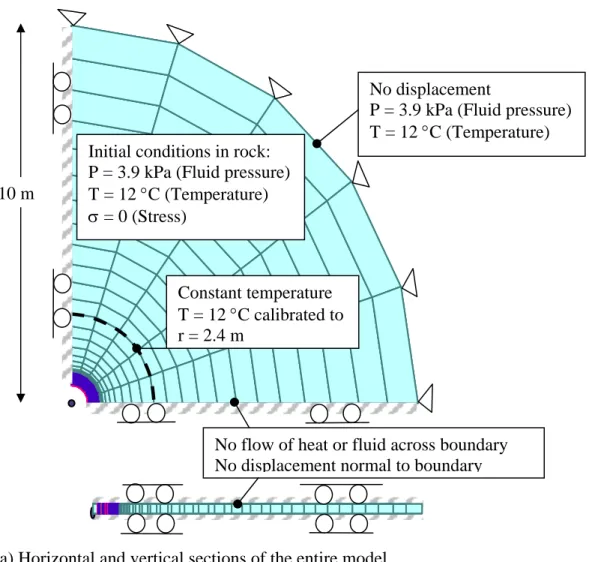
In this section, the re-evaluation of the Kamaishi THM experiment is presented by using a simplified axisymmetric model (cf. Fig. 1.12), with the boundary conditions and locations of output points shown in Fig. 3.25. Simulation was performed both in the heating phase (258 days) and the cooling phase (180 days).
Figure 3.25: Model geometry and boundary conditions
3.4.2 Parameters for simulation
Many parameters of bentonite were obtained by laboratory tests directly (Fujita et al., 1997). The water diffusivity is a function of volumetric water content and temperature. The water potential is a function of volumetric water content. These relationships were determined by laboratory tests. The thermal water diffusivity and parameters for swelling pressure were determined by back analysis of laboratory test. Furthermore, the thermal expansion coefficient is newly calibrated.
C L
52cm 85cm
1000cm
Steel Bentonite
Rock No flow of heat or fluid across boundary No displacement normal to boundary
No displacement P=3.9kPa T=12ºC Constant temperature T = 12ºC calibrated to r = 2.5m 47cm T = 100ºC during heating