https://doi.org/10.15626/MP.2018.869 Article type: Tutorial
Published under the CC-BY4.0 license
Open materials: Yes Open and reproducible analysis: Yes Open reviews and editorial process: Yes
Preregistration: Not applicable
S.R. Martin, C.O. Brand Analysis reproduced by: André Kalmendal All supplementary files can be accessed at OSF: https://osf.io/v2pnc/
A fully automated, transparent, reproducible,
and blind protocol for sequential analyses
Brice Beffara Bret
LPPL - EA 4638, Université de Nantes, Nantes, France
Laboratoire de psychologie - EA 3188, Université de Franche-Comté, Besançon, France
The Walden III Slowpen Science Laboratory, Villeurbanne, France
Amélie Beffara Bret
LPPL - EA 4638, Université de Nantes, Nantes, France
The Walden III Slowpen Science Laboratory, Villeurbanne, France
Ladislas Nalborczyk
Department of Experimental Clinical and Health Psychology, Ghent University, Belgium
The Walden III Slowpen Science Laboratory, Villeurbanne, France
Abstract
Despite many cultural, methodological, and technical improvements, one of the major obstacle to results repro-ducibility remains the pervasive low statistical power. In response to this problem, a lot of attention has recently been drawn to sequential analyses. This type of procedure has been shown to be more efficient (to require less obser-vations and therefore less resources) than classical fixed-N procedures. However, these procedures are submitted to both intrapersonal and interpersonal biases during data collection and data analysis. In this tutorial, we explain how automation can be used to prevent these biases. We show how to synchronise open and free experiment software programs with the Open Science Framework and how to automate sequential data analyses in R. This tutorial is intended to researchers with beginner experience with R but no previous experience with sequential analyses is required.
Keywords: Sequential analysis, Sequential testing, Sequential Bayes factor, Automation, Expectancy effects,
Repro-ducibility, Blind analyses
On reproducibility
It may be referred to as a crisis, a revolution, or a
renaissance, but Psychology has undeniably known a
decade of unparalleled methodological reflection and
reform (for an overview, see Fidler & Wilcox,2018; Nel-son et al., 2018). Although many of the practices that are currently recognised as part of the problem (e.g., poor understanding of statistical methods, questionable
research practices) have long been acknowledged (e.g., Babbage, 1830),1 recently introduced practices have
brought considerable improvements to the reliability of findings in psychological science (e.g., see Smaldino et al.,2019).
There are many ways to define what reproducibility is, and it is often unclear what is meant by the terms of reproducibility, replicability, repeatability, or reliability. To avoid these confusions, we adopt the terminology suggested by Goodman et al. (2016). When discussing research reproducibility, we make a distinction between i) methods reproducibility: the ability to reproduce, as closely as possible, the methodological procedures de-veloped by a certain team (i.e., what is usually meant by reproducibility), ii) results reproducibility: the ability to reproduce a certain result in a given methodologi-cal settings (i.e., what is usually meant by replicability), and iii) inferential reproducibility: the ability (for an in-dependent team) to replicate an inferential conclusion, that is, to arrive at the same conclusion.
Whereas results reproducibility concerns the out-come of a computational or experimental procedure, methods reproducibility is a property of the methods be-ing used to produce this particular outcome. As put by Meehl (1990), a scientific study is akin to a recipe, and a good methods description should allow other cooks to prepare the same kind of cake as the person that wrote the recipe did. As such, methods reproducibility is essential to results reproducibility. Fortunately, recent technical developments have made the task far easier than it used to be. Key components of a modern repro-ducible workflow may include:
• Transparency: exhaustive and intelligible descrip-tion and sharing of all materials, scripts, etc. (for a practical introduction, see Klein et al.,2018)
• Self-containment: writing reproducible
docu-ments in LaTeX or RMarkdown (e.g., see
the R package papaja, Aust & Barth, 2018)
and sharing self-contained code (e.g., see
https://codeocean.com)
• Version control: using Git and Github (or Gitlab) to track changes in working documents (for an in-troduction, see Vuorre & Curley,2018)
• Automation: minimising mistakes by automatis-ing as many steps of the research process as pos-sible (e.g., Rouder, 2016; Rouder et al., 2018; Yarkoni et al.,2019)
Although methods reproducibility is essential to re-sults reproducibility, it is not sufficient. Despite having
a long history of scrutiny in Psychology, one of the ma-jor threats to results reproducibility remains statistical power, where power can be broadly defined as the prob-ability of achieving a certain goal, given that a suspected underlying state of the world is true (Kruschke,2015). We know that a low powered result has (all other things being equal) a lower probability to replicate, the initial result being attached with a higher probability of erro-neous inference (e.g., type-M or type-S errors, Gelman & Carlin, 2014). Even though there are many ways to increase statistical power (e.g., see Hansen & Collins,
1994), we focus here on sequential testing, that is, the continuous analysis of data during its collection. This procedure has been shown to optimise the amount of resources (e.g., money and time) to be spent in order to attain a certain goal, as compared to classical a priori power analyses strategies (Lakens,2014; Schönbrodt et al.,2017).
We turn now to a brief presentation of several se-quential analyses procedures, followed by a discussion of the methodological precautions that need to be un-dertaken to ensure the validity of these procedures. Fi-nally, we outline the core aspects of a "born-open" (fol-lowing the terminology of Rouder, 2016), fully auto-mated, and reproducible workflow for sequential anal-yses.
A brief introduction to sequential analyses procedures
In this section, we briefly introduce three sequential analysis procedures that address three distinct goals. More precisely, these procedures permit to either i) ac-cumulate relative evidence for a hypothesis (the
sequen-tial Bayes factor procedure) or ii) efficiently accept or
reject a value or range of values for a parameter (the sequential HDI+ROPE procedure) or iii) sample obser-vations until a desired level of estimation precision is reached.
Sequential Bayes factor
Schönbrodt et al. (2017) presented an alternative to null-hypothesis significance testing with a priori power analysis (NHST-PA) by introducing the Sequential Bayes
Factor (SBF) procedure. The SBF procedure uses Bayes
factors (BFs) to iteratively examine the relative eviden-tial support for a hypothesis during data collection.2
1Where the same could be said for recently proposed
so-lutions like preregistration or radical transparency (e.g., de Groot,2014).
2Technically speaking, the Bayes factor is a ratio of
marginal likelihoods (i.e., what is considered as evidence in the Bayesian framework). Broadly, a BF can be interpreted
The first step of the SBF procedure is to pick thresh-olds (one for each of the two hypotheses being com-pared) that determine the end of data collection. These thresholds should be selected to reflect the level of evi-dence that the experimenter consider sufficient to stop data collection, but should also be defined in consider-ation of specific goals and costs-benefits analyses. In-deed, more stringent thresholds require larger sample sizes, but are associated with lower risks of misleading inferences (false positive and false negative), all other things being equal. Then, after picking the appropriate prior distribution for the alternative hypothesis, a first batch of observations is collected, during which no BF is computed (to avoid misleading inferences due to early terminations). Starting at nmin observations (the a
pri-ori defined minimum sample size), a BF is computed at each stage (or each observation). The sampling proce-dure goes on until the current BF reaches the a priori de-fined threshold or until reaching nmaxobservations (the
a priori defined maximum sample size).
Schönbrodt et al. (2017) provided detailed simu-lation results of this procedure when comparing the means of two independent groups (the equivalent of a two-samples t-test). They show that the error rates and the average length of the procedure (i.e., how many observations are needed to reach the threshold) are a function of both the population effect size, the thresh-old, and the prior for the alternative hypothesis. For instance, when chasing a medium effect size (d = 0.5) and when using a "medium scaled" prior for the alterna-tive (r = 1), stopping data collection at BF = 6 instead of BF= 3 results in a percentage of wrong inferences of 4.6% instead of 40% (see Table 1 in Schönbrodt et al.,
2017, p. 10).
Based on these results, it is possible to combine prior guesses or expectations with the known properties of the SBF procedure to design experiments. This strategy is known as design analysis and includes the classical power analyses of the NHST framework as a particu-lar case. In this vein, Schönbrodt and Wagenmakers (2018) introduced the Bayes Factor Design Analysis tool and demonstrated how this strategy can help to design more informative empirical studies (see also Stefan et al.,2019).
The sequential HDI+ROPE procedure
Bayes factors are not the only available option to per-form sequential testing. Whereas BFs quantify the ev-idence in favour of an hypothesis (relative to another hypothesis), each individual hypothesis can also be ex-amined on its own. For instance, the hypothesis that the group difference of some measured variable is equal to zero might be assessed by looking directly at the
pos-terior distribution of the group difference.3 This
dis-tribution can be summarised via its mean and highest
density interval (HDI), an interval that contains the X%
most credible values for the parameter (Kruschke & Lid-dell, 2018).4 The hypothesis according to which the
group difference is equal to zero can then be assessed by checking whether the HDI includes zero as a credible value. Alternatively, and more interestingly, the HDI can be compared to a region of practical equivalence (ROPE, Kruschke,2018), defining the range of effect sizes that we consider as negligible (i.e., equivalent to zero) for practical purposes.
The comparison of HDI and ROPE can be summarised by computing the proportion of the HDI that is included in the ROPE, giving an idea of the extent to which the hypothesis of no effect is supported. Alternatively, the comparison of the HDI to the ROPE can result in three categorical outcomes: i) the null hypothesis is rejected (when the HDI falls completely outside the ROPE), ii) the null hypothesis is accepted (when the HDI falls
com-pletely inside the ROPE), or iii) the data is said to be
inconclusive (when neither of the above applies). When the goal of the analysis is to accept or reject a reference value, it is then possible to stop data collec-tion when the HDI does not include this reference value. Thus, this procedure is similar to the SBF procedure, except that the sampling procedure is terminated by a (conclusive) comparison of a HDI to a ROPE, instead of being terminated by a comparison of a BF value to some threshold (for a detailed study of the characteristics of this procedure, see Kruschke,2015).
Aiming for precision
Because data collection stops when the accumulated evidence reaches a certain threshold, sequential hy-pothesis testing procedures (e.g., SBF or HDI+ROPE) are known to be biased by extreme observations. In other words, the data collection stops when the col-lected data supports the hypothesis, preventing the op-portunity of collecting contradictory data afterwards as an updating factor, indicating how credibility should be re-allocated from prior knowledge (what was known before seeing the data) to posterior knowledge (what is known after seeing the data).
3The posterior distribution is the result of any Bayesian
analysis. It is a probability distribution that allocates prob-ability to parameter values, given the model (including the priors) and the observed data.
4The HDI is a particular type of credible interval, the
Bayesian equivalent of the frequentist confidence interval. It should be noted however that the interpretation of Bayesian and frequentist intervals differ considerably (e.g., Morey et al.,
(Kruschke, 2015). Performing sequential analysis un-til a certain estimation precision is reached overcomes this bias (Kruschke,2015). In this procedure, the goal is not to stop data analysis based on the rejection of an hypothesis but rather to sample observations until a predefined level of precision in a parameter (including effect size) estimation is reached. The estimation pre-cision can be quantified by the width of the HDI and Kruschke (2015) proposes to stop data analysis when the HDI width is less than 80% of the ROPE’s width. For instance, if the smallest effect size of interest (SESOI, Lakens et al., 2018) is δ = 0.2, we can define a ROPE around 0 from δ = −0.1 to δ = 0.1. This means that we will consider an effect as approximately null when it is less than half our SESOI. Planing for precision, we would therefore stop data collection when the width of our HDI (on the estimate of the effect size) is inferior to 0.8 × 0.2= 0.16 (Kruschke,2018).
Of course, there are other methods to determine the desired level of precision. For instance, researchers can base their SESOI on an effect of minimal clinical rele-vance. In this context, the SESOI varies depending on the costs and benefits of the treatment (Lakens et al.,
2018). We can also imagine other criteria to determine precision on the basis of the ROPE. In any case, even if one wants to check whether the HDI falls inside the ROPE at the end of data collection, planing for precision enables us to focus on parameter or effect size estima-tion instead of hypothesis testing. If we decide to plan for moderate precision, we will not need a large amount of observations, but it is likely that the HDI will overlap the ROPE. As a consequence, it will not be possible to reach a categorical conclusion. If we plan for high preci-sion, more observations will be needed to stop data col-lection, but hypothesis testing will be improved as well as precision. In most situations, planing for precision will require more observations than hypothesis testing.
Whatever the procedure, the stopping rule should be thought carefully by considering and balancing the costs and benefits of collecting more observations. A small number of observations is affordable but likely to lead to biased conclusions. A large number of observations can be expensive but likely to lead to more robust con-clusions. Both frequentist and Bayesian methods have their ways to deal with risks and errors in sequential hypothesis testing. Criteria are modified for sequential hypothesis testing so that "significant" p-values (e.g., .0294 instead of .05 for one interim analysis, Lakens,
2014) or Bayes factors (e.g., BF = 6 instead of BF = 3 depending on acceptable error rates, Schönbrodt et al.,2017) are not the same as classical (non sequential) hypothesis testing. This should also be considered in sequential the HDI+ROPE procedure.
Some difficulties
The procedures previously described and discussed in Schönbrodt et al. (2017) and Kruschke (2015,2018) offer an attractive perspective on data collection. How-ever, some precautions need to be undertaken in order to preserve a good precision or the long-term error rates they provide. More precisely, we discuss two main cat-egories of biases that need to be controlled. We call the first category of biases intrapersonal biases, as bi-ases that are expressed within individuals. These bibi-ases mainly emerge during data analysis and data reporting. We call the second category of biases interpersonal
bi-ases, as biases that are expressed between individuals.
These biases mainly emerge during data collection (e.g., when the researcher interacts with participants).
These biases can arise in any study but sequential procedures present specific risks on both the intra and interpersonal dimensions. We explain why in the next section.
What could possibly go wrong? Intrapersonal biases during sequential analyses
Most intrapersonal biases occur because of what some would call the "researcher degrees of freedom" (Simmons et al.,2011; Wicherts et al.,2016). Following Wicherts et al. (2016)’ nomenclature, we identified the following intrapersonal biases as having increased risks in sequential procedures:
• C3: Correcting, coding, or discarding data during
data collection in a non-blinded manner.
• A1: Choosing between different options of
deal-ing with incomplete or missdeal-ing data on ad hoc grounds.
• A2: Specifying pre-processing of data (e.g.,
clean-ing, normalization, smoothclean-ing, motion correc-tion) in an ad hoc manner.
• A3: Deciding how to deal with violations of
statis-tical assumptions in an ad hoc manner.
• A4: Deciding on how to deal with outliers in an
ad hoc manner.
These degrees of freedom allow flexibility when pro-cessing data before statistical inference. This flexibility can be dangerous when incentives, cultural norms, or previous practices influence data analysis, and where there are few safeguards. Thus, the intrapersonal na-ture of these biases does not refer to an absence of so-cial influence, but rather to biases occurring at the point where the researcher makes choices on her own. This
can be the case when someone discards an outlier to reach a significant result because it is easier to pub-lish with significant results. This can also be the case when one tries different data transformations to best match their preferred hypothesis. Here the problem-atic nature of the degrees of freedom is the researcher’s subjectivity. Discarding an outlier or transforming data is not necessarily the result of being an outlier or be-ing skewed data, but can also be the result of what the researcher wants to see because of economic, so-cial (e.g., reputation pressure), cultural contexts. These biases are not specific to sequential procedures but their consequences might be amplified during sequential pro-cedures because of the possible impact of each look at the data. Indeed, the degrees of freedom can impact data analysis at time t1 which can in turn impact data
collection in a self-perpetuating cycle. Data analysis at time t2is therefore likely to be biased by the degrees of
freedom at time t2 but also at time t1. Thus, errors
ac-cumulate because the effects of the degrees of freedom are multiplied.
When a data analyst has expectations about what should be observed, the data analysis is likely to be biased by these expectations through confirma-tion (favouring an hypothesis) or disconfirmaconfirma-tion (stronger scepticism toward data against the hypothesis than toward data corroborating the hypothesis) biases (MacCoun & Perlmutter, 2017). While continuously analysing data, the data analyst is faced with many choices about the best way to deal with incoming data. Based on previous studies, they might have expectations about the range of plausible values, or they might need to use particular methods to process physiological sig-nals, to recode or to transform data in a specific way, and so on. We urge researchers to make these decisions explicit before data collection.
The properties of sequential procedures have been studied extensively via simulation (Kruschke, 2015; Schönbrodt et al., 2017; Wagenmakers et al., 2017). However, noise and irregularities in simulated data only come from sampling variability, and not from practi-cal problems that can be encountered during empiripracti-cal data collection (e.g., technical issues or experimenter biases). When collecting data, researchers would like to get as close as possible to the shape of simulated data (i.e., we would like to minimise other sources of errors than sampling variability). In order for the BF, the HDI or the precision to be reliable stopping crite-ria, they have to be computed on reliable data. We ac-knowledge that what can be considered as reliable data heavily depends on the type of study. As such, decisions concerning the analysis workflow should be justified by the existing literature as much as possible. However,
changing the criterion and methods for data prepara-tion based on the state of the sequential procedure is not acceptable. The result of an experiment cannot de-termine the way it is itself defined. Real-time result-hacking would jeopardise the confidence one can have in this result.
Therefore, we propose that all the steps of the se-quential procedure (i.e., data preparation and cleaning, outliers detection, data transformation, model assump-tions checks, and data analysis) should be automated and performed in an incremental manner. The entire dataset can be continually reanalysed, including former outliers, so that the process follows the progressive in-corporation of new observations. Put more formally, such a procedure should be able to take into account that an extreme observation at time t might not be ex-treme anymore at time tn, and should therefore be
re-included in subsequent analyses.
The fact that this iterative procedure is automated should prevent the data analyst from the hazards that are commonly encountered during data manipulation (see previous section). These hazards have particu-larly important consequences in sequential procedures in comparison to traditional (i.e. fixed-n) procedures because of the incremental nature of evidence accumu-lation. A specific preprocessing choice at time t can influence inference criteria computation at time t+n which can subsequently influence another preprocess-ing choices and so on. With accumulated modifications in preprocessing decisions, the inference criteria are not only computed based on data but also on sequential and incremental choices from the scientist. We propose that these steps could instead be programmed and coded on the basis of preregistered choices, before starting to col-lect data. Preregistered automated data analysis would therefore ensure conclusions based on empirical proce-dures to be similar to the results (e.g., long-term er-ror rates) provided by Schönbrodt et al. (2017) or Kr-uschke (2015) using simulation, and explicitly fulfil the requirements of transparency and reproducibility.
However, being able to define in advance the goal and the criteria for success of these sequential proce-dures requires i) to be well aware of the literature of interest, ii) to know how data behave by manipulat-ing data from very similar previous experiments or pre-tests, iii) to be able to implement a procedure of data preparation for model computation before seeing new data. These three points might seem trivial but are even more important for sequential analyses than classical procedures in order to avoid intermediate influences in data preparation based on known interim results.
In addition to these intermediate influences (i.e., in-fluences between the collection of the first batch of data
and the final data analysis) in data preparation, inter-mediate influences can also be problematic during data collection. These influences are what we call "interper-sonal biases".
Interpersonal biases during sequential analyses
By interpersonal biases we refer to biases that might occur when a researcher interacts with participants during data collection. According to Wicherts et al. (2016)’s nomenclature, the interpersonal bias with po-tentially increased risks in sequential procedures is:
• C2: Insufficient blinding of participants and/or
experimenters.
When an experimenter has expectations about what should be observed, data collection is likely to be bi-ased by these expectations (Gilder & Heerey, 2018; Klein et al.,2012; Orne,1962; Rosenthal,1963; Rosen-thal,1964; Rosenthal & Rubin,1978; Zoble & Lehman,
1969). One solution to prevent this bias is to make sure that experimenters are blind to the experimental condi-tions.
Double blind5 designs are expected to minimise
ex-pectancy effects (Gilder & Heerey, 2018; Klein et al.,
2012). However, when the experimenter cannot be
blind, expectancy effects are to be expected. This bias has been clearly identified by Lakens (2014) as a partic-ularly strong risk (i.e. observer effects are likely to be stronger in the context of sequential testing) in sequen-tial analysis: "Experimenter bias is important to con-sider when performing a study under normal circum-stances [...] but becomes even more important to con-sider when the experimenter has performed an interim analysis."
What is the specific status of sequential testing con-cerning analyst and observer expectancy effects? Ex-pectancy effects arise when one has prior beliefs and/or motivations about the outcome of an experiment and involuntarily (we assume scientific honesty) influences the results on the basis of these prior beliefs and motiva-tions. The confidence in a hypothesis can be influenced by previous results from the literature, naive representa-tions about the studied phenomenon, and other sources of information. These sources may deal with the studied phenomenon but rarely with the ongoing study specif-ically, and, as a consequence, the potential hypothesis can be subject to uncertainty. When performing sequen-tial testing, one has a direct access to the accumulation of evidence concerning the ongoing study. Hence, the prior information accumulated from sequential analy-sis specifically reduces uncertainty about the potential results of the ongoing experiment as compared to in-formation gathered from previous studies or naive
rep-resentations. In other words, a bias toward a particu-lar result may stem from previous literature or personal beliefs. In the sequential analysis context, a bias to-ward a particular result may also stem from observing the accumulating data across the sequential procedure. This could be particularly strong, because one can di-rectly see the accumulated data as the sample size in-creases in real time. Knowing about intermediate re-sults can therefore increase the risk of falling into an "evidence confirmation loop". In the previous section, we proposed that this risk applies to confirmation and disconfirmation biases (data analysis) where the intrap-ersonal bias of data evaluation can inflate with accumu-lated evidence. In this section, we propose that this loop can also worsen experimenter expectancy effects during data collection. The interpersonal bias of experimenter-participant interactions can be seen as a self-fulfilling prophecy amplified by feedback from previous data.
Clearly, it is very difficult to obtain robust results concerning the effect size of analyst and observer ex-pectancy effects. Indeed, one would have to carry out experiments on experiments in order to study these bi-ases. This "meta-science" problem is arduous because these biases can apply at all levels of manipulation as one experiment is included in another. For instance, Barber (1978) suggested that expectancy biases can also occur in the expectancy bias research. It can also be dif-ficult to collect large observation samples by experimen-tal conditions (e.g., Zoble & Lehman, 1969), although recent work has shown that it was possible (Gilder & Heerey, 2018). Thus, we can only draw attention to these effects as a potential risk to consider rather than as a precisely quantified danger to avoid.
When double blind designs are not practicable,
in-terpersonal biases seem obvious. However, when a
double blind design is set up, the existence of an in-terpersonal bias is probably more questionable. How could knowledge about previous data influence the out-come of the experiment? It is possible that the exper-imenter’s verbal and non-verbal motor cues impact on the participant’s behaviour (Zoble & Lehman, 1969). However, it is unlikely that only non-verbal cues un-derlie the experimenter expectancy effect, at least in simple or familiar tasks (Hazelrigg et al., 1991). What we know today is that the experimenter expectancy ef-fect can be inadvertent and can depend on the inter-action between the experimenter and the participant (Gilder & Heerey, 2018; Hazelrigg et al., 1991). Per-sonality variables such as the need of social influence (on the experimenter’s side) and the susceptibility to
5We use the "double blind" terminology according to the
classical definition, where both the participant and the exper-imenter are blind to the experimental condition.
social influence (on the participant’s side) can also in-crease the expectancy bias (Hazelrigg et al.,1991). In a double-blind design however, the experimenter can-not influence the participant’s responses on the basis of knowledge of the experimental condition. However, the (de)motivation and the disappointment/satisfaction of seeing the preferred hypothesis contradicted/confirmed by the sequential testing procedure can possibly influ-ence the participant.6 We cannot rule out the
possi-bility that the confidence in a hypothesis interacts with experimental conditions and impacts the results of the experiment in one way or another. Because the exper-imenter is not aware of the experimental condition of the participants, they will probably influence them more uniformly than in a simple blind design. This means that the behaviour of the experimenter can potentially change the baseline value of a parameter in all partici-pants. Also, we cannot exclude the possibility that the effect of the experimental manipulation is biased by this baseline value shift. More generally, "contextual vari-ables, such as experimenters’ expectations, are a source of error that obscures the process of interest" (Klein et al.,2012).
What could be expected?
To the best of our knowledge, there is no experiment reporting expectancy biases when the experimenter is blind to the experimental condition. However, blinding the experimenter from interim analysis is certainly rec-ommended (Lakens,2014) when blinding experimental conditions is not possible. We suggest that blinding the analysis should also be considered as a precaution, even when the experimenter is blind.
In Table1, we describe hypothetical observable con-sequences of such biases on the SBF and HDI+ROPE procedures. Importantly, expectation biases can emerge in all combinations of a priori expectations and pop-ulation effect sizes. Congruent observations are ex-pected to increase the speed with which the threshold is reached (H0+ and H1+), whereas incongruent ob-servations are expected to slow down this process (H0-and H1-) (H0-and to increase the number of false alarms.
Evidence is insufficient to conclude on the practical significance of analyst and observer expectancy effects, especially in double blind designs. If the necessary methods to reduce bias were costly and the potential benefits uncertain, then it would be reasonable to be sceptical of our proposal. However, we will show in the next section that the methods required to reduce bias are easy to implement, and therefore costless to adopt.
We have presented how the knowledge of previous data can bias the data collection process and have also
illustrated the predicted consequences of these biases on the evolution of sequentially computed BFs. In the next section, we focus on how to prevent these biases from happening. We suggest two ways of implementing analysis blinding as a precaution against experimenter biases during sequential testing, and present a proof of concept for an automated procedure that would ensure objectivity.
A fully automated, transparent, reproducible and triple-blind protocol for sequential testing
Blinding is the procedure which hides the assigned condition from people involved in the experiment. It can notably be applied to participants, experimenters, or data analysts (Schulz & Grimes,2002). If possible, it is preferable to apply blinding to anyone involved in the experiment to avoid expectancy effects. Whereas partic-ipant and experimenter blinding is often considered in Psychology, much less attention has been given to anal-ysis blinding, probably due to materials and time con-straints. However, the use of analysis blinding would help eliminate some of the biases identified in Wicherts et al. (2016). Again, this has been well described by Lakens (2014): "In large medical trials, tasks such as data collection and statistical analysis are often assigned to different individuals, and it is considered good prac-tice to have a data and safety monitoring board that is involved in planning the experiment and overseeing any interim analyses. In psychology, such a division of labor is rare, and it is much more common that researchers work in isolation".
Analysis blinding can take two different forms in the context of sequential analyses procedures. First, analy-sis blinding can refer to a procedure ensuring that the person analysing the data is blind to the hypotheses (Miller & Stewart,2011). This configuration minimises intrapersonal biases because the analyst does not have the information necessary to influence data analysis in a specific direction (congruent or incongruent with the hypothesis). Second (and more specifically to sequen-tial testing procedures), analysis blinding can refer to a procedure ensuring that the experimenter is blinded to the data analysis. This configuration minimises inter-personal biases because the experimenter does not have the information necessary to influence data collection in a specific direction (congruent or incongruent with the hypothesis).
If the experimenter is not the data analyst, they can be blind to the evolution of the intermediate results un-til data collection stops. As a consequence, the specific
6Ideally, scientists should be interested in all possible
Table 1
Possible interactions between the population value of the effect size and the a priori expectations of the experimenter during a (non-blind) sequential testing procedure.
There is no difference in the population (H0: δ= 0)
There is a difference in the population (H1: δ , 0)
Researcher 1, believes in H0 H0+ (congruent) H1- (incongruent) Researcher 2, believes in H1 H0- (incongruent) H1+ (congruent)
experimenter expectancy bias in the sequential proce-dure is avoided. Another solution is to automate anal-ysis blinding so that the data analyst and the experi-menter (who can be the same person) are blind to in-termediate results computed on previous sets of obser-vations. To illustrate this idea, we describe below how to perform transparent blind sequential analysis. We propose an example for two independent-groups com-parisons (as in Schönbrodt et al.,2017). This tutorial covers all experimental steps from preregistration to re-sults reporting. When several options are available for a specific step, we detail one in the manuscript and other possibilities in the supplementary materials. We provide a functional example of the procedure on the OSF (Open Science Framework) based on an emo-tional Stroop experiment. In order to describe the pro-cedure, we use the idea of Rouder (2016) who took the perspective of his dog Kirby to explain Git and Github. Here we take the perspective of Lisa Loud,7 who loves
carrying out experiments but has probably never used automated sequential analysis before.
Prerequisites
• Lisa needs to have an Open Science Framework (OSF,https://osf.io/register/) account.
• Lisa needs to have at least some basic knowledge about how to use the OSF. See Soderberg (2018) and https://help.osf.io/ for a practical introduc-tion.
• Lisa needs to have R (R Core Team, 2019) and RStudio (https://www.rstudio.com/) installed on her computer.
• Lisa needs to have a recent version of OpenS-esame (https://osdoc.cogsci.nl/) or PsychoPy (https://www.PsychoPy.org/) installed on her computer.
"Born-open" data
The aim of this this tutorial is not to discuss the the-oretical work necessary before carrying out an
experi-ment. We will directly focus on the preparation of ma-terials needed to collect data.
This tutorial mainly deals with computerised exper-iments.8 In this situation, users need to program an
experiment to collect data. The logic proposed here is compatible with experiments programmed with Psy-choPy (Peirce, 2007, 2008; Peirce et al., 2019) or OpenSesame (Mathôt et al.,2012). These software pro-grams have the advantage of being free and able to com-municate with the OSF. These two qualities are crucial for transparent procedures and easy sharing.
We will use the possibility to link the software program with the OSF in order to propose an intuitive "born-open" data procedure (Rouder, 2016). Although OSF synchronisation tools are generally easy to install on Windows and Mac OS, it can be slightly more "complicated" on other operating systems (OS) such as Linux OS. Most users probably work on Windows and Mac OS. However, because Linux OSs are free and open we believe that they fit well with the open
science philosophy. Consequently, we will provide
minimal examples on how to use this tutorial on Ubuntu as a popular and easy-to-use Linux distribution.
We propose a procedure using OpenSesame be-low. Procedures with PsychoPy can be found in the
supplementary materials. OpenSesame probably allows the simplest synchronisation with the OSF. How-ever, it is less flexible than PsychoPy for programming experiments because, unlike PsychoPy, it does not allow to access to a coder view. Direct OSF synchronisation is available with PsychoPy 2 but not with PsychoPy 3. The example available on the OSF is based on PsychoPy 2 but has also been successfully tested with OpenSesame. Table2proposes a summary of the main strengths and weaknesses of each method.
Programming the experiment for "born-open" data. We present how to program an experiment
al-7https://theloudhouse.fandom.com/wiki/Lisa_Loud 8However, some parts of the proposed protocol can be
Table 2
Global overview of open experiment programming software’s characteristics and synchronisation handling.
OpenSesame
PsychoPy 2
PsychoPy 3
Synchronisation
OSF
OSF
Pavlovia and Gitlab*
Automatic synchronisation ease
+
-
-Graphical interface for synchronisation
++
-
++
Synchronisation quality
++
+
+++
Software flexibility
-
++
++
*Indirect synchronisation is possible with OSF because synchronisation is possible between OSF and Gitlab. Direct synchronisation
with OSF could also be possible but probably not straightforward.
lowing automatic "born-open" data with OpenSesame, currently the easiest way to program automatic "born-open" data. For more flexibility in experiment pro-gramming, PsychoPy options are described in the
supplementary materials. OpenSesame is "a graphi-cal experiment builder for the social sciences". It is free, open-source, and cross-platform. It features "a compre-hensive and intuitive graphical user interface and sup-ports Python scripting for complex tasks." (Mathôt et al.,
2012). OSF integration is normally included by default for Windows and Mac OS. If not (or for other OS like Ubuntu for instance), the installation procedure is de-scribed in the supplementary materials. If OSF in-tegration is installed, the user should see the OSF icon in OpenSesame (Figure 1). Click the OSF log-in but-ton and sign in with your OSF account. More details on OSF integration in OpenSesame can be found at
https://osdoc.cogsci.nl/3.1/manual/osf/. If Lisa reads this part of the manual, she will know exactly what to do in order to link data to the OSF.9If she links data to the OSF, each time that data has been collected (nor-mally after every experimental session), this data is also uploaded to the OSF. Lisa should follow the following steps in order to do so:
• Lisa has to save the experiment on her computer. • She then has to open the OSF explorer, right-click
on the folder that she wants the data to be up-loaded to, and select "Sync data to this folder". The OSF node that the data is linked to will be shown at the top of the explorer.
• She finally needs to check "Always upload col-lected data" and data files will be automatically saved to OSF after they have been collected.
Script preparation and piloting
Performing sequential analyses requires strict exper-iment programming and data analysis preparation.
Be-Figure 1. OSF log-in button in the main toolbar in
OpenSesame
cause data is continuously analysed during data collec-tion, everything must be ready before collecting data. This can be seen as a disadvantage because there is a lot of work to be done before data collection. Indeed, analysing data after data collection allows us to delay several choices thus allowing to launch data collection more quickly.10However, this can also be considered as
a huge advantage because there are no unexpected sur-prises after data collection. It is not possible to discover that something has not been recorded or that data is not in the appropriate format, or that data is more dif-ficult to analyse than expected. Everything is thought about upstream because everything must work for data analysis which is performed during data collection. We propose this 6-step procedure to prepare the analysis:
• Clearly define the variables involved in the study
9The following part is a reformulation of the manual for
the purpose of our tutorial.
10Here we do not say that preparation is specific to
sequen-tial testing. Preparation can be recommended for all designs, but is not avoidable in sequential analysis.
in order to program the experiment
• Carefully consider how to analyse the data to be collected
• Program the experiment in keeping with the planned data analysis
• Test the experiment to check that everything is working as expected
• Prepare the scripts that will be used to analyse data
• Run some pilots to test the procedure
These steps are necessary in order to launch the ac-tual experiment. Otherwise, sequential analyses are likely to fail at some point.
Preregistration
Let’s assume Lisa has successfully achieved script preparation and piloting. When everything is ready, she has everything she needs to preregister her study. Preregistration is very important in sequential testing because it forces Lisa to explicitly state her statistical criteria of interest and therefore announce when data collection will end. This is very useful in order to limit biases due to Lisa’s degrees of freedom (Lakens,2014; Wicherts et al.,2016).
In addition to generic preregistration, the first impor-tant thing to preregister is the sequential data clean-ing procedure. In this part, Lisa should describe how data will be handled before inferential statistical mod-elling. This can include, physiological signal process-ing, potential observation or participant removal crite-ria or any other data manipulation happening between data collection and modelling. After that, Lisa should indicate the appropriate stopping statistics depending on the procedure (e.g., SBF, HDI+ROPE, precision). The stopping statistic should be described along with a clear and detailed description of the model which is computed to get this statistic. Finally, Lisa should also specify a minimum sample size required to compute the models, and a maximal sample size affordable for her, which would determine the end of data collection, in-dependently of the stopping statistic.
Transparent data collection
When possible, making data openly available can im-prove the quality of science (Klein et al.,2018). In the context of sequential data analysis, it can be even more important. As we explained above, sequential analyses offer strong advantages but also increase Lisa’s degrees of freedom. Making data open can reduce this bias. In
this perspective, born open data (Rouder,2016) can be even more efficient, especially in the context of sequen-tial analysis. "Born-open" data is the procedure which makes data automatically open as soon as it is collected. This procedure has at least two huge interests for se-quential analysis. First, the time course of data collec-tion is transparent because data is necessarily sent on-line and time-stamped just after being collected. This is very important because in doing so, each choice made by Lisa will be clear and justified. Second, "born-open" data will facilitate real time online data analysis which is very useful for sequential designs. automatic "born-open" data is possible with OpenSesame or PsychoPy by automatic publishing data on the OSF (or on Github or Gitlab for instance).
Automated data cleaning
After collecting her first batch of data, Lisa might not be able to directly fit the statistical model she is inter-ested in. She probably needs a procedure of data clean-ing in order to get her data ready for statistical infer-ence. Data cleaning can include physiological signal processing, artefacts removal, errors removal, dealing with potential outliers, and everything needed to get meaningful data from raw data. Lisa has to perform data cleaning before statistical modelling. Because Lisa is analysing data sequentially, she also has to clean data sequentially.
For instance, in our example (the emotional Stroop task), we decided to remove missing data and response
times (RT) below 100 ms. This is done each time
new data is incorporated (see lines 101 to 110 of the
sequential_analyses.R script). We could also have
chosen to analyse RT only for correct responses and/or to remove observations based on a specific descriptive statistic.
Automated blind data analysis
Because Lisa has prepared everything needed for her procedure, she is able to automate data analysis and therefore to be blind to the details of the analysis while she is collecting data. Here is how she can proceed and how we proceeded in our example.
We describe how Lisa can handle tasks-scheduling on a UNIX system (macOS and Linux) in this
para-graph. Lisa can use the cronR package (Wijffels,
2018a) to schedule tasks in R. This package will be useful in order to retrieve data from the OSF and to analyse it. Lisa will have to create a task by run-ning the appropriate script (main_script.R in our ex-ample) once before collecting the first observation. She will be able to decide how often she wants the script to run automatically. Lisa could also apply
the same procedure on a Windows system thanks to the taskscheduleR package (Wijffels, 2018b). A short description on how to use this package can be found at: https://cran.r-project.org/web/packages/ taskscheduleR/vignettes/taskscheduleR.html.
If Lisa chooses that the script should auto-run each hour, the main script will check data from the OSF each hour. This will be done with the osfr package (Wolen & Hartgerink,2019). In our example (Line 106 to 143 in main_script.R), we check if new data is available on the OSF and download it if it is the case. After some data formatting (lines 145 to 197), the script will run the sequential analysis (line 199 to 243). The main script calls the sequential_analyses.R script which contains the sequential analyses function. Lisa will also have to specify some parameters depending on the model she is interested in.
At the end of the analysis, Lisa will receive an email telling her whether to stop or to continue data collec-tion. This email will neither report the effect nor its di-rection, but only the information to stop or to continue the data collection. This means that Lisa will be able to follow a sequential design without any information about the results of data analysis, excepted the fact that she has (not) reached her criterion. The mail will be sent automatically in R thanks to the gmailR package (Hester,2016).
Reproducible reporting
Lisa will stop data collection when she reaches her statistical criterion or her maximum affordable sample size. She will then be able to write a report describing her results. She can do it using RMarkdown (Allaire et al.,2019; Xie et al.,2018) in order to incorporate her results automatically from her R scripts into her report (e.g., see Bauer,2018). Lisa could for instance use the R package papaja (Aust & Barth, 2018) which would allow her to write a reproducible APA manuscript with RMarkdown. Scientific writing with Rmarkdown has important benefits for any type of research design but would be even more valuable for sequential analyses.
Feasibility of the proposed protocol and limitations
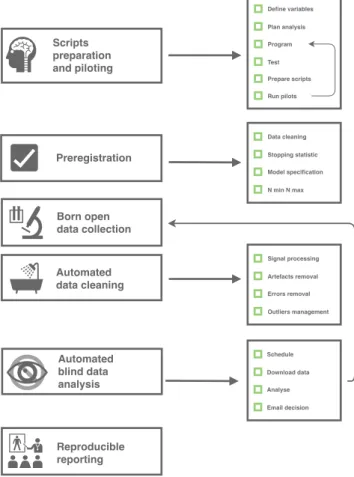
A graphical summary of the procedure is depicted in Figure2.11All the tools needed to set it up are available
for free to everyone. Using OpenSesame or PsychoPy is relatively straightforward and does not necessarily require coding skills. We proposed standard R scripts in order to automate sequential analysis. However, we concede that using this scripts requires minimal knowl-edge of R. Hence, we also propose a Shiny applica-tion available athttps://barelysignificant.shinyapps.io/ blind_sequential_analyses/. With this application, Lisa
would just have to specify all the important details of her analysis in boxes, from which the application gen-erates the corresponding R script almost ready for se-quential analysis. This application is meant to facilitate the creation of R scripts. It automatically writes around 90% of the code Lisa would have to write to use such a sequential analysis procedure. However, it is almost certain that the produced R code would not work imme-diately. It would require some minor tweaking from her, such as checking the local path, making sure that the scripts and the data are in the same repository, adapting the data import step to specific properties of the data under consideration, and so on.
The procedure proposed here only requires one com-puter. Hence, the implementation cost is rather low. This procedure is also well suited for multi-lab studies. Indeed, an experiment can be run at different places but data is automatically centralised on one platform and can be analyse automatically and sequentially by one single computer. The experiment we designed with PsychoPy 2 (see the supplementary material for more information) is specifically thought for multi-lab studies by automatically recording information about the com-puter which runs the experiment. This enables the iden-tification of the site associated with each participant.
We concede that automation of data analysis prevents one interesting advantage of sequential testing. Namely, the fact that data collection can be stopped whenever the behaviour of data is unexpected, allowing the ex-perimenter to rethink the experimental design or aim before collecting more data (Lakens,2014). Depending on the confidence and expected familiarity with the data to be collected, the researchers have to choose between automated or "two-person" analysis blinding. The first option has low costs of implementation whereas the sec-ond one is more flexible. In any case, after performing a sequential analysis, nothing prevents Lisa from perform-ing additional analyses based on unexpected data speci-ficity, taking care to record and state the exploratory nature of any such analyses.
A word on blind analysis by multiple people
If Lisa can afford working with a colleague on her study and if she prefers to do so, we advise her to ap-ply the logic of the automated procedure described in this tutorial. The only difference will be that her col-league will analyse data while Lisa collects it (or con-versely). If her colleague analyses data, they will have to retrieve data online (e.g., on OSF) and to perform the planned preregistered analysis (unless data behave
11This figure has been inspired by the Figure 1 in Quintana
Figure 2. Schematic procedure of a transparent and
blind sequential data analysis.
Define variables Plan analysis Program Test Prepare scripts Run pilots Data cleaning Stopping statistic Model specification N min N max Signal processing Artefacts removal Errors removal Outliers management Preregistration Scripts preparation and piloting Born open data collection Automated data cleaning Automated blind data analysis Reproducible reporting Schedule Download data Analyse Email decision
very unexpectedly in which case they will have the re-sponsibility to adapt the analysis or stop data collection prematurely). The only contact Lisa and her colleague will have concerning the experiment will be the email they will send to inform Lisa whether to stop or con-tinue data collection, nothing more.
Conclusions
We began by presenting the intra and interpersonal biases that might emerge during sequential testing and sequential analysis procedures. To tackle these issues, we proposed a novel automated, transparent, repro-ducible and blind protocol for sequential analysis. The main interest of this procedure is to reduce possible biases that could be encountered during intermediate data analysis and to prevent the inflation of social influ-ences during data collection.
This protocol should be considered as a proof-of-concept for sequential analysis automation. However, future work will be able to propose more comprehensive and more user-friendly solutions for sequential
analy-ses. For instance, the reliance on the user’s R program-ming skills might be alleviated with the development of an online platform that would automate the procedure online, without the need for coding.
More work is also needed to precisely quantify in-tra and interpersonal biases during data collection and analysis. For instance, one could set up experimental procedures to pinpoint these biases in realistic lab sit-uations (e.g., see Gilder & Heerey, 2018). In addition to experimental procedures, computational modelling could also be used to estimate the presence of bias in ex-tant (published or not) sequential analyses. By formalis-ing the sequential analysis procedure (e.g., usformalis-ing an evi-dence accumulation model) and by explicitly modelling the biases that we describe in the present article, we might be able to assess the likelihood that an observed set of collected statistics (e.g., BFs) has been obtained under the assumption of bias (or no bias).
Supplementary materials
Reproducible code and supplementary materials are available on OSF:https://osf.io/mwtvk/.
Author Contact
Correspondence concerning this article should be addressed to Brice Beffara Bret, Université de Nantes, Nantes, France. E-mail: brice.beffara@univ-nantes.fr.
ORCID: Brice Beffara Bret https://orcid.org/
0000-0002-0586-6650 - Amélie Beffara Bret
https://orcid.org/0000-0002-9129-0415 - Ladislas Nalborczykhttps://orcid.org/0000-0002-7419-9855
We thank Hans IJzerman for helpful comments and Edward Collett for his help with manuscript English proof reading on a previous version of this manuscript. Many thanks to Christopher Moulin for his feedback and for his help with manuscript English proof reading on the updated version of this manuscript. We also thank Rickard Carlsson, Félix Schönbrodt, Angelika Stefan, Stephen Martin, and Charlotte Brand for insightful comments and suggestions during the peer-review process.
Conflict of Interest and Funding
The authors report no conflict of interest. We thank the Université de Nantes, the Université Grenoble Alpes, and the Université de Franche-Comté for supporting our research. The author(s) received no specific financial support for the research, authorship, and/or publication of this article.
Author Contributions
Following the CRediT – Contributor Roles Taxonomy (https://casrai.org/credit/):
Conceptualisation: BBB (lead), ABB, LN Data curation: BBB, LN
Formal analysis: LN Investigation: BBB, ABB Methodology: BBB, ABB, LN
Project administration: BBB, ABB, LN Resources: BBB, ABB, LN
Software: BBB (OpenSesame, PsychoPy, Python), LN (R) Validation: BBB, ABB, LN
Visualisation: BBB, ABB, LN Writing: BBB, ABB, LN
Authorship order was determined as follow (by order of significance):
- First author: original idea and major contribution to the "software" role (inter alia)
- Last author: major contribution to the "software" role (inter alia)
- Second author: major contribution to the "investiga-tion" role (inter alia)
Open Science Practices
This article earned the Open Data and the Open Ma-terials badge for for making the data and maMa-terials openly available. It has been verified that the analy-sis reproduced the results presented in the article. The entire editorial process, including the open reviews, are published in the online supplement.
References
Allaire, J., Xie, Y., McPherson, J., Luraschi, J., Ushey, K., Atkins, A., Wickham, H., Cheng, J., Chang, W., & Iannone, R. (2019). Rmarkdown: Dynamic
documents for r [R package version 1.12].https:
//rmarkdown.rstudio.com
Aust, F., & Barth, M. (2018). papaja: Create APA
manuscripts with R Markdown [R package
ver-sion 0.1.0.9842]. https : / / github . com / crsh / papaja
Babbage, C. (1830). Reflections on the decline of science
in England, and on some of its causes. B.
Fel-lowes [etc.]
Barber, T. X. (1978). Expecting expectancy effects: Bi-ased data analyses and failure to exclude al-ternative interpretations in experimenter ex-pectancy research. Behavioral and Brain
Sci-ences, 1(03), 388.https : / / doi . org / 10 . 1017 /
S0140525X00075531
Bauer, P. C. (2018). Writing a Reproducible Paper in R Markdown. SSRN Electronic Journal. https : / / doi.org/10.2139/ssrn.3175518
de Groot, A. (2014). The meaning of “significance” for different types of research [translated and an-notated by Eric-Jan Wagenmakers, Denny Bors-boom, Josine Verhagen, Rogier Kievit, Marjan Bakker, Angelique Cramer, Dora Matzke, Don Mellenbergh, and Han L. J. van der Maas]. Acta
Psychologica, 148, 188–194. https : / / doi . org /
10.1016/j.actpsy.2014.02.001
Fidler, F., & Wilcox, J. (2018). Reproducibility of Sci-entific Results. In E. N. Zalta (Ed.), The
Stan-ford Encyclopedia of Philosophy (Winter 2018).
Metaphysics Research Lab, Stanford University. Gelman, A., & Carlin, J. (2014). Beyond power calcula-tions: Assessing type s (sign) and type m (mag-nitude) errors. Perspectives on Psychological
Sci-ence, 9(6), 641–651.https://doi.org/10.1177/
1745691614551642
Gilder, T. S. E., & Heerey, E. A. (2018). The Role of Ex-perimenter Belief in Social Priming.
Psycholog-ical Science, 29(3), 403–417.https://doi.org/
10.1177/0956797617737128
Goodman, S. N., Fanelli, D., & Ioannidis, J. P. A. (2016). What does research reproducibility mean?
Sci-ence Translational Medicine, 8(341), 341ps12.
https://doi.org/10.1126/scitranslmed.aaf5027
Hansen, W. B., & Collins, L. M. (1994). Seven Ways To Increase Power Without Increasing N [type: dataset]. NIDA research monograph, 142, 184– 195. https://doi.org/10.1037/e495862006-008
Hazelrigg, P. J., Cooper, H., & Strathman, A. J. (1991). Personality moderators of the experimenter ex-pectancy effect: A reexamination of five hy-potheses. Personality and Social Psychology
Bul-letin, 17(5), 569–579. https : / / doi . org / 10 .
1177/0146167291175012
Hester, J. (2016). Gmailr: Access the gmail restful api [R package version 0.7.1]. https : / / CRAN . R -project.org/package=gmailr
Klein, O., Doyen, S., Leys, C., Magalhães de Saldanha da Gama, P. A., Miller, S., Questienne, L., & Cleeremans, A. (2012). Low Hopes, High Ex-pectations: Expectancy Effects and the Replica-bility of Behavioral Experiments. Perspectives on
Psychological Science, 7(6), 572–584. https : / / doi.org/10.1177/1745691612463704
Klein, O., Hardwicke, T. E., Aust, F., Breuer, J., Daniels-son, H., Hofelich Mohr, A., Ijzerman, H., Nil-sonne, G., Vanpaemel, W., & Frank, M. C. (2018). A Practical Guide for Transparency in Psychological Science. Collabra: Psychology,
4(1), 20.https : / / doi . org / 10 . 1525 / collabra .
158
Kruschke, J. K. (2015). Doing Bayesian data analysis:
A tutorial with R, JAGS, and Stan (Edition 2).
Academic Press.
Kruschke, J. K. (2018). Rejecting or Accepting Parame-ter Values in Bayesian Estimation. Advances in
Methods and Practices in Psychological Science,
1(2), 270–280. https : / / doi . org / 10 . 1177 /
2515245918771304
Kruschke, J. K., & Liddell, T. M. (2018). The Bayesian New Statistics: Hypothesis testing, estimation, meta-analysis, and power analysis from a Bayesian perspective. Psychonomic Bulletin &
Review, 25(1), 178–206.https : / / doi . org / 10 .
3758/s13423-016-1221-4
Lakens, D. (2014). Performing high-powered studies ef-ficiently with sequential analyses: Sequential analyses. European Journal of Social Psychology,
44(7), 701–710.https://doi.org/10.1002/ejsp.
2023
Lakens, D., Scheel, A. M., & Isager, P. M. (2018). Equiv-alence Testing for Psychological Research: A Tu-torial. Advances in Methods and Practices in
Psy-chological Science, 1(2), 259–269.https://doi.
org/10.1177/2515245918770963
MacCoun, R. J., & Perlmutter, S. (2017). Blind Anal-ysis as a Correction for Confirmatory Bias in Physics and in Psychology. In S. O. Lilienfeld & I. D. Waldman (Eds.), Psychological Science
Un-der Scrutiny (pp. 295–322). John Wiley & Sons,
Inc.https://doi.org/10.1002/9781119095910. ch15
Mathôt, S., Schreij, D., & Theeuwes, J. (2012). OpenS-esame: An open-source, graphical experiment builder for the social sciences. Behavior
Re-search Methods, 44(2), 314–324. https : / / doi .
org/10.3758/s13428-011-0168-7
Meehl, P. E. (1990). Appraising and Amending Theo-ries: The Strategy of Lakatosian Defense and Two Principles that Warrant It. Psychological
In-quiry, 1(2), 108–141. https : / / doi . org / 10 .
1207/s15327965pli0102\_1
Miller, L. E., & Stewart, M. E. (2011). The blind leading the blind: Use and misuse of blinding in ran-domized controlled trials. Contemporary
Clini-cal Trials, 32(2), 240–243.https://doi.org/10.
1016/j.cct.2010.11.004
Morey, R. D., Hoekstra, R., Rouder, J. N., Lee, M. D., & Wagenmakers, E.-J. (2016). The fallacy of plac-ing confidence in confidence intervals.
Psycho-nomic bulletin & review, 23(1), 103–123.https:
//doi.org/10.3758/s13423-015-0947-8
Nalborczyk, L., Bürkner, P.-C., & Williams, D. R. (2019). Pragmatism should not be a substitute for sta-tistical literacy, a commentary on albers, kiers, and van ravenzwaaij (2018). Collabra:
Psychol-ogy, 5(1). https://doi.org/10.1525/collabra.
197
Nelson, L. D., Simmons, J., & Simonsohn, U. (2018). Psychology’s Renaissance. Annual Review of
Psy-chology, 69(1), 511–534. https://doi.org/10.
1146/annurev-psych-122216-011836
Orne, M. T. (1962). On the social psychology of the psychological experiment: With particular ref-erence to demand characteristics and their im-plications. American psychologist, 17(11), 776– 783.https://doi.org/10.1037/h0043424
Peirce, J. W. (2007). PsychoPy—Psychophysics soft-ware in Python. Journal of Neuroscience
Meth-ods, 162(1-2), 8–13.https://doi.org/10.1016/
j.jneumeth.2006.11.017
Peirce, J. W. (2008). Generating stimuli for neuro-science using PsychoPy. Frontiers in
Neuroinfor-matics, 2.https://doi.org/10.3389/neuro.11.
010.2008
Peirce, J. W., Gray, J. R., Simpson, S., MacAskill, M., Höchenberger, R., Sogo, H., Kastman, E., & Lin-deløv, J. K. (2019). PsychoPy2: Experiments in behavior made easy. Behavior Research
Meth-ods, 51(1), 195–203.https://doi.org/10.3758/
s13428-018-01193-y
Quintana, D., Alvares, G., & Heathers, J. (2016). Guidelines for reporting articles on psychiatry and heart rate variability (graph): Recommen-dations to advance research communication.
Translational psychiatry, 6(5), e803. https : / /
doi.org/10.1038/tp.2016.73
R Core Team. (2019). R: A language and environment for
statistical computing. R Foundation for
Statisti-cal Computing. Vienna, Austria.https://www. R-project.org/
Rosenthal, R. (1963). On the social psychology of the psychological experiment: The experimenter’s hypothesis as unintended determinant of ex-perimental results. American Scientist, 51, 268– 283.
Rosenthal, R. (1964). Experimenter
experiment. Psychological Bulletin, 61(6),
405–412.https://doi.org/10.1037/h0045850
Rosenthal, R., & Rubin, D. B. (1978). Interpersonal ex-pectancy effects: The first 345 studies.
Behav-ioral and Brain Sciences, 1(03), 377. https : / /
doi.org/10.1017/S0140525X00075506
Rouder, J. N. (2016). The what, why, and how of born-open data. Behavior Research Methods, 48(3), 1062–1069. https://doi.org/10.3758/s13428-015-0630-z
Rouder, J. N., Haaf, J. M., & Snyder, H. K. (2018). Minimizing Mistakes In Psychological Science.
PsyArXiv. https : / / doi . org / 10 . 31234 / osf. io /
gxcy5
Schönbrodt, F. D., & Wagenmakers, E.-J. (2018). Bayes factor design analysis: Planning for compelling evidence. Psychonomic Bulletin & Review.https: //doi.org/10.3758/s13423-017-1230-y
Schönbrodt, F. D., Wagenmakers, E.-J., Zehetleitner, M., & Perugini, M. (2017). Sequential hypothe-sis testing with Bayes factors: Efficiently test-ing mean differences. Psychological Methods,
22(2), 322–339. https : / / doi . org / 10 . 1037 /
met0000061
Schulz, K. F., & Grimes, D. A. (2002). Blinding in randomised trials: Hiding who got what. The
Lancet, 359(9307), 696–700.https://doi.org/
10.1016/s0140-6736(02)07816-9
Simmons, J. P., Nelson, L. D., & Simonsohn, U. (2011). False-Positive Psychology: Undisclosed Flexibil-ity in Data Collection and Analysis Allows Pre-senting Anything as Significant. Psychological
Science, 22(11), 1359–1366.https://doi.org/
10.1177/0956797611417632
Smaldino, P., Turner, M. A., & Contreras Kallens, P. A. (2019). Open science and modified funding lot-teries can impede the natural selection of bad science. https : / / doi . org / 10 . 31219 / osf . io / zvkwq
Soderberg, C. K. (2018). Using OSF to Share Data: A Step-by-Step Guide. Advances in Methods
and Practices in Psychological Science, 1(1),
115–120. https : / / doi . org / 10 . 1177 / 2515245918757689
Stefan, A. M., Gronau, Q. F., Schönbrodt, F. D., & Wa-genmakers, E.-J. (2019). A tutorial on Bayes Factor Design Analysis using an informed prior.
Behavior Research Methods, 51(3), 1042–1058.
https://doi.org/10.3758/s13428-018-01189-8
Vuorre, M., & Curley, J. P. (2018). Curating Research As-sets: A Tutorial on the Git Version Control Sys-tem. Advances in Methods and Practices in
Psy-chological Science, 1(2), 219–236. https://doi.
org/10.1177/2515245918754826
Wagenmakers, E.-J., Marsman, M., Jamil, T., Ly, A., Ver-hagen, J., Love, J., Selker, R., Gronau, Q. F., Šmíra, M., Epskamp, S., Matzke, D., Rouder, J. N., & Morey, R. D. (2017). Bayesian infer-ence for psychology. Part I: Theoretical advan-tages and practical ramifications. Psychonomic
Bulletin & Review, 25(1), 35–57. https : / / doi .
org/10.3758/s13423-017-1343-3
Wicherts, J. M., Veldkamp, C. L. S., Augusteijn, H. E. M., Bakker, M., van Aert, R. C. M., & van Assen, M. A. L. M. (2016). Degrees of Freedom in Planning, Running, Analyzing, and Reporting Psychological Studies: A Checklist to Avoid p-Hacking. Frontiers in Psychology, 7.https://doi. org/10.3389/fpsyg.2016.01832
Wijffels, J. (2018a). Cronr: Schedule r scripts and
pro-cesses with the ’cron’ job scheduler [R package
version 0.4.0]. https : / / CRAN . R - project . org / package=cronR
Wijffels, J. (2018b). Taskscheduler: Schedule r scripts
and processes with the windows task scheduler
[R package version 1.4.0]. https : / / CRAN . R -project.org/package=taskscheduleR
Wolen, A., & Hartgerink, C. (2019).
Osfr: R interface to osf
[http://centerforopenscience.github.io/osfr, https://github.com/centerforopenscience/osfr]. Xie, Y., Allaire, J., & Grolemund, G. (2018). R
markdown: The definitive guide [ISBN
9781138359338]. Chapman; Hall/CRC. https:
//bookdown.org/yihui/rmarkdown
Yarkoni, T., Eckles, D., Heathers, J., Levenstein, M., Smaldino, P., & Lane, J. I. (2019). Enhancing and accelerating social science via automation: Challenges and opportunities.https://doi.org/ 10.31235/osf.io/vncwe
Zoble, E. J., & Lehman, R. S. (1969). Interaction of sub-ject and experimenter expectancy effects in a tone length discrimination task. Behavioral
Sci-ence, 14(5), 357–363. https : / / doi . org / 10 .