different playstyles
Master Thesis Project 15p, Spring 2020
Author:
Tadas Ivanauskas
ivanauskas15@gmail.com
Supervisors:
Jose Maria Font
Fernanderz
Examiner:
Johan Holmgren
Contact information
Author:
Tadas Ivanauskas
E-mail: ivanauskas15@gmail.com
Supervisors:
Jose Maria Font Fernanderz E-mail: jose.font@mau.se
Malm¨o University, Department of Computer Science and Media Technology.
Examiner: Johan Holmgren
E-mail: johan.holmgren@mau.se
Abstract
The number of features and number of instances has a significant impact on computation time and memory footprint for machine learning algorithms. Reducing the number of features reduces the memory footprint and compu-tation time and allows for a number of instances to remain constant. This thesis investigates the feature reduction by clustering.
9 clustering algorithms and 3 classification algorithms were used to investi-gate whether categories obtained by clustering algorithms can be a replace-ment for original attributes in the data set with minimal impact on classifi-cation accuracy.
The video game Blood Bowl 2 was chosen as a study subject. Blood Bowl 2 match data was obtained from a public database The results show that the cluster labels cannot be used as a substitute for the original features as the substitution had no effect on the classifications. Furthermore, the cluster labels had relatively low weight values and would be excluded by activation functions on most algorithms.
Popular science summary
You are not playing a hybrid, you are just bad at the game.
Blood Bowl 2 community has long argued about what race falls into what category. Finally, the answer is here. Quite a few community members tried to objectively group races by playstyles, the closest we got was arguing on online message boards. This time we used 200 000 matches and asked the machines to do it for us.
By looking at meters run, stuns, blocks, passes and other numbers, machine learning algorithms found three playstyles, namely bash, dash and hybrid. The interesting difference between these playstyles is that hybrid performs worse than the other two at nearly everything.
The races do not neatly fall into categories, more like they lean towards their categories. This means that it is possible to play bash with elves and play dash with dwarves, but chances of winning the match drop significantly. The findings of this paper can provide some insight for the developers to balance the races and help the community to formulate better strategies for their preferred races.
Acknowledgment
Special thanks to Kamilla Klonowska for finding time to provide feedback and support. Also, many thanks to Jose Maria Font Fernandez and Alberto Enrique Alvarez Uribe for the topic idea and for setting me on the correct path. Finally thanks to Andreas Harrison who provided help and support for gathering the data that was used in this research.
Contents
1 Introduction 11
1.1 Background . . . 11
1.2 Motivation . . . 12
1.3 Aim and Objectives . . . 13
1.4 Research Questions . . . 14
1.5 Chapter Summary . . . 15
2 Related work 16 2.1 Sports Games Modeling . . . 16
2.2 Machine Learning . . . 17
2.3 Data Preprocessing . . . 23
2.4 Chapter Summary . . . 25
3 Preliminaries: Blood Bowl 2 26 3.1 Terminology . . . 26 3.2 Game Description . . . 27 3.3 Player Statistics . . . 27 3.4 Races . . . 28 3.5 Match Statistics . . . 29 3.6 Chapter Summary . . . 30 4 Proposed Approach 31 4.1 Data Acquisition . . . 31 4.2 Data Preparation . . . 32 4.3 Number of Clusters . . . 33
4.4 Chapter Summary . . . 35 5 Method 36 5.1 Motivation . . . 36 5.2 The Experiment . . . 37 5.3 Measurements . . . 37 5.4 Algorithms . . . 39 5.5 Chapter Summary . . . 41 6 Results 42 6.1 Clustering Results . . . 42 6.2 Classification Results . . . 56 6.3 Chapter Summary . . . 61
7 Analysis and Discussion 62 7.1 Clustering Analysis . . . 62
7.2 Generalization . . . 64
7.3 Classification Analysis . . . 66
7.4 Validity Threats and Limitations . . . 67
7.5 Chapter Summary . . . 67
8 Conclusion and Future Work 68 8.1 Conclusion . . . 68 8.2 Future Work . . . 70 8.3 Chapter Summary . . . 70 9 Appendices 77 9.1 Source Code . . . 77 9.2 Heat-map . . . 77 9.3 PCA Figures . . . 79 9.4 Clustering Figures . . . 82
List of Figures
2.1 Visualization of K- means clustering. . . 18
2.2 Scree plot showing relationship between number of clusters and sum of squared errors. . . 19
2.3 Example dendrogram (right) clustering six data points. . . 21
2.4 Mean shift centroid movement. . . 22
2.5 Fitting and transforming the data using PCA. . . 25
3.1 Races in Blood Bowl 2 Legendary edition. . . 28
4.1 Explained variance using 34 attributes containing 24 compo-nents. . . 33
4.2 Elbow method showing 3 clusters. . . 34
6.1 Race dendrograms displaying three clusters obtained trough hierarchical clustering. . . 43
6.2 K-Means Clustering results. . . 44
6.3 K- means Silhouette index. . . 45
6.4 Affinity propagation clustering results. . . 46
6.5 Silhouette index for affinity propagation clustering. . . 46
6.6 BIRCH clustering results. . . 47
6.7 Silhouette index for BIRCH clustering. . . 48
6.8 Spectral clustering results. . . 49
6.9 Silhouette index for spectral clustering. . . 49
6.10 DBSCAN clustering results. . . 50
6.12 OPTICS clustering results. . . 52
6.13 Silhouette index for OPTICS clustering. . . 52
6.14 Gaussian clustering results. . . 53
6.15 Silhouette index for Gaussian clustering. . . 54
6.16 Mean Shift clustering results. . . 55
6.17 Silhouette index for mean shift clustering. . . 55
7.1 Box plot showing passes for each cluster. . . 63
7.2 Experience statistics for each cluster. . . 64
7.3 Breaks for each race. . . 65
9.1 Heat-map depicting the similarity between features. . . 78
9.2 Explained variance using 34 attributes containing 24 compo-nents. Full size figure. . . 80
9.3 Elbow method showing 3 clusters. Full size figure. . . 81
9.4 Race dendrograms displaying three clusters obtained trough hierarchical clustering. Full size figure. . . 83
9.5 K-Means Clustering results. Full size figure. . . 84
9.6 Affinity propagation clustering results. Full size figure. . . 85
9.7 BIRCH clustering results. Full size figure. . . 86
9.8 Spectral clustering results. Full size figure. . . 87
9.9 DBSCAN clustering results. Full size figure. . . 88
9.10 OPTICS clustering results. Full size figure. . . 89
9.11 Gaussian clustering results. Full size figure. . . 90
List of Tables
2.1 Example data that is to be grouped by animal. . . 24
2.2 Data from previous table grouped by animal. . . 24
5.1 Clustering algorithms that are tested in this study. . . 40
6.1 Overview of clustering results . . . 56
6.2 Classification results. . . 57
6.3 Gaussian Naive Bayes Confusion matrix . . . 57
6.4 Logistic Regression Confusion matrix . . . 57
6.5 SVC Confusion matrix . . . 58
6.6 Feature weights for classification algorithms. . . 59
List of Acronyms
BIRCH Balanced Iterative Reducing and Clustering using Hierarchies CSV Comma Separated Values
DBSCAN Density-Based Spatial Clustering of Applications with Noise JSON JavaScript Object Notation
OPTICS Ordering Points To Identify the Clustering Structure PCA Principal Component Analysis
SVC Support Vector Classification XML Extensible Markup Language
Chapter 1
Introduction
This chapter introduces the thesis work and frames it within the context of existing work. The following subchapters describe the topic, how it relates to computer science, and states motivations for conducting the research. Aims and objectives are explicitly expressed, research questions are presented and described in this chapter.
1.1
Background
This thesis is based on, and a continuation of previous research on a simi-lar topic by Andreas Gustafsson [1]. Their research attempts to predict the winner of the video game Blood Bowl 2 using machine learning classification algorithms. Gustafsson used the data set constructed from a publicly avail-able database that contains log data of game matches. The research included grouping the game races by their playstyle. The categories were constructed using statistical analysis by a community member by the name of Schlice [2]. The Schlice research lacks validity, critical analysis and is just a blog post. The races appear to shift categories when several leagues of the game are analyzed. This thesis work employs machine learning algorithms to cluster the races by their playstyles using game log files acquired over the span of five months. A. Gustafsson emphasized the importance of the coaches (hu-man actors) while this study ignores the hu(hu-man factor altogether. Hu(hu-man
actors are strictly limited by the rules of the game of which there are plenty [3, 4]. Grouping races and play styles by coach proved to be challenging for A. Gustafsson due to most coaches having played very small amounts of games. A. Gustafsson also mentioned that using a deep neural network was not possible due to long training times. This research will attempt to reduce the number of features in the original data set. Feature selection for machine learning has been an important problem and there are several techniques proposed [5, 6]. By adding the categories for races and playstyles it might be possible to reduce the number of features in the data set thus speeding up the learning time for the classifiers.
Previous work [1] focused on the coach (human actor) while this work puts more emphasis on the players (the game figures) and the importance of races. The motivation is that there are proposed several playstyles and certain races lean towards those playstyles. Playstyles can possibly counter each other and the playstyle and race of the players have more weight over the human ac-tor. Coach skill is a factor in individual games, however over the multiple games and different coaches should even out. Outlier cases such as one of the races being significantly more powerful than any other race can skew the results. Knowledgeable coaches would naturally choose the powerful races more often. The opposite outlier case is possible as well. One race being significantly under-powered would mean that knowledgeable coaches would avoid it, while lesser skilled coaches still choose it.
1.2
Motivation
Clustering groups data points by identifying similarities and provides a higher-level overview of the data in a given set. This thesis proposes a novel feature reduction method that uses high-level abstraction obtained through cluster-ing to replace low-level features in the original data set. Clustercluster-ing has been used as a feature reduction technique, however, it was used as a replacement for principal component analysis (PCA) [7, 8, 9]. This thesis proposes a technique to use clustering in conjunction with PCA to reduce the number of features with minimal impact on the classification performance.
Additionally, this thesis identifies the playstyles present in the Blood Bowl 2 game and provides a scientific basis for it. Currently proposed playstyles lack validity and are based on community opinions.
1.3
Aim and Objectives
The main goal of this thesis is to reduce the number of features in the data set using clustering algorithms. To achieve this goal, the study aims to abstract related features behind cluster labels with minimal impact on classification results.
Additionally, the study aims to deepen the understanding of the Blood Bowl 2 match dynamic as well as overarching strategies employed in those matches. The community of Blood Bowl 2 outlined three major strategies used in the game namely bash, dash, and hybrid, however, there is little research done on the subject. This thesis aims to provide the clearly defined categories in which every Blood Bowl 2 race could be placed as well as a scientific basis for the resulting categories. This would help the community to understand the game mechanics better and provide the developers of the game with more information about the interactions that happen in different matches. Cat-egorizing the playstyles will provide valuable information on how to cluster and categorize highly complex and overlapping data points.
Following objectives are established to help achieve the thesis goal:
Examine and test various clustering algorithms to establish possible categories for the playstyle of each race.
Analyze the data set and incorporate the playstyles for each match. Select important features in the data set.
1.4
Research Questions
The research question is set for the thesis is: Can categorizing entries in the data set, obtain the playstyles, improve the classification accuracy for winner prediction in Blood Bowl 2 game? However, this research question is too broad and open-ended therefore is split into several more concrete and close-ended questions which are:
RQ1 How machine learning can be used to categorize races and extract playstyles from complex and varying data such as Blood Bowl 2 match log files?
RQ2 How does clustering performance differ between different clustering al-gorithms and how it can be measured?
RQ3 How categories obtained through clustering algorithms affect the per-formance of classification algorithms?
RQ4 Can categories obtained through clustering algorithms be a replace-ment for original attributes in the data set with minimal impact on the accuracy of the classifier?
The first research question analyzes clustering algorithms and clusters match data from Blood Bowl 2 games. The clustering might require feature selec-tion to narrow down the distribuselec-tion of the data points. The second research question will examine different clustering algorithms to understand what are their benefits and what clustering strategies they employ. This research ques-tion will compare the clustering algorithms to determine which algorithms cluster the data effectively and produce the best silhouette indexes for clus-tering Blood Bowl 2 races. The third research question incorporates resulting categories into the existing data set which is later classified to obtain the pre-diction of the game outcomes. The fourth research question examines the data set and determines what features (if any) can be replaced by newly constructed categories obtained by answering RQ2.
1.5
Chapter Summary
This chapter introduced the study and the motivations for why it is im-portant to pursue the knowledge regarding academic as well as community aspects. Mainly to combine PCA and clustering to further reduce the num-ber of features. Clustering was used as a feature reduction method, however, it was viewed as a replacement for PCA.
This chapter clearly stated the research questions and supporting aims and objectives. These objectives provided help in outlining the experiment. The proposed experiment is to preprocess the data using PCA, cluster the result-ing set, and use the clusterresult-ing labels with the original data set to predict the winner of matches.
Chapter 2
Related work
The first part of the proposed experiment in this study is to use machine learning algorithms to identify the playstyles in the Blood Bowl 2 matches. This chapter introduces the reader to state-of-the-art knowledge regarding machine learning and data preparation. Sub-chapters delve deeper into clus-tering algorithms. This chapter also introduces data preparation including grouping, normalization, and Principal Component Analysis.
2.1
Sports Games Modeling
This paper treats the Blood Bowl 2 video game as a test subject. The video game is based on real sports games and has elements of the fantasy world. Real football games are not bound by the limitations set by the programmer and are more complex due to a high number of agents present during the match and can be affected by third parties and disruptions from outside the game field. The Blood Bowl 2 video game allows one person to control the team which drastically reduced the complexity of games.
Statistical analysis and machine learning is a powerful tool that is being used in sports as a means to predict the outcome of each match [10, 11], model the player movement [12] or even model the players to provide advice for the managers on forming the team [13]. Machine learning is being used to determine what makes a team stand out from the rest through clustering
[14] and whenever passing or rushing is a better feature in determining the strength of the team [15].
Blood Bowl 2 being a video game, naturally has more restrictions of what can happen during the match, this alleviates a lot of problems that mentioned papers encountered. Although it is not possible to translate the results from previously mentioned publications, it is possible to loosely adapt the ap-proach and methods used in the research.
2.2
Machine Learning
Machine learning is a broad field that is based on statistical data analysis. Large amounts of data are used to derive features, models, and patterns in the data without explicit need to be hard coded. There are several types of machine learning, but the most important two in this research are super-vised and unsupersuper-vised learning. Machine learning algorithms build internal models from the training data and then uses those models to produce out-puts for the new input data. Supervised learning matches the input data to predefined labeled output and it is most commonly used for classification problems such as in [1] where there are a set number of possible outputs. Unsupervised learning does not have predefined outputs and is commonly used for clustering problems such as presented in this thesis [16].
2.2.1
Clustering
Clustering algorithms attempt to find similarities between the data inputs by grouping them together [17]. This approach allows to simplify the complex data and categorizes the input values. It also provides more detailed insight into the data set. In our case, clustering algorithms are used to uncover underlying playstyles in BloodBowl 2. There are several approaches to solve clustering problems, each of them has its benefits and shortcomings. Below are short explanations of clustering algorithms used in this research.
2.2.2
K - means Clustering
K - means clustering is one of the most popular clustering algorithms and it is fairly simple in its implementation. The algorithm first assigns the cen-troids to the data (figure 2.1 b). Cencen-troids can be chosen at random or they can be placed on top of existing data points. Poorly chosen centroid can result in slow performance or bad clustering [18]. Python machine learning library sklearn provides “k - means ++” clustering where initial centroids are spread far away from each other resulting in better and more consistent performance [19]. The algorithm then assigns the data points to the closest centroid (figure 2.1 c) and centroids are moved to the mean of the data points for that cluster (figure 2.1 d, e). This process is repeated a set number of times or until the centroid is no longer being moved (figure 2.1 f).
Figure 2.1: Visualization of K- means clustering.
Source: https://stanford.edu/~cpiech/cs221/handouts/kmeans.html K - means clustering algorithm requires the number of clusters to be known before the learning process can take place, this is referred to as
hyperparam-eter. If the data set is fairly simple, the number of clusters can be observed visually as in figure 2.1 a. If the data set contains more than three di-mensions, it cannot be visualized and requires mathematical understanding. Hyperparameter tuning is one of the solutions to this problem. The number of clusters can be found by clustering the data set for different numbers of clusters and calculating the sum of the squared distances between centroids. Plotting the relationship between error and the number of clusters produces a curve graph where an increase in the number of clusters reduces the clus-tering error. The optimal number of clusters is the elbow of the curve [20] [21] (figure 2.2). The elbow point denotes the breakpoint were further in-creasing the number of clusters yields minimal gains and therefore judged as not worth the extra computational resources. Furthermore, increasing the number of cluster can cause the over fitting problem where each data point is assigned it‘s own cluster.
Figure 2.2: Scree plot showing relationship between number of clusters and sum of squared errors.
Source: https://www.researchgate.net/figure/
Result-of-the-elbow-method-to-determine-optimum-number-of-clusters_ fig8_320986519
2.2.3
Hierarchical Clustering
Hierarchical clustering generates clusters of clusters [22]. When hierarchi-cal clustering is represented as a tree structure, each node is considered as a cluster when the algorithm starts. The algorithm calculates dissimilarity between the clusters and assigns the values for it. The most similar clusters are merged into one cluster and the process is repeated until all the data points are enclosed in one big cluster. Hierarchical clustering results are pre-sented in dendrograms (figure 2.3). One axis displays the data points while the other displays dissimilarity between those points. Dissimilarity can be measured as the distance between the data points as shown in the figure 2.3. Hierarchical clustering works well with fewer data points as the biggest downside of the method is its scalability. Large sets of data are hard to read and analyze using dendrograms and hierarchical clustering.
Dissimilarity in our case is measured in euclidean distance between the data points. There are several ways to merge the data together. Single linkage measures the distance between two data points that are closest together, average linkage calculates the clusters average resulting in a centroid and measures the distance between cluster centroids. Complete linkage mea-sures the distance between the furthest two data points. The choice in The linkage is performance-oriented rather than accuracy-oriented [23]. Different linkages result in similar clusters, but the order of the data points is different.
Figure 2.3: Example dendrogram (right) clustering six data points. Source: https://www.displayr.com/what-is-dendrogram/
2.2.4
Affinity Propagation Clustering
Affinity propagation clustering is similar to hierarchical clustering. This algorithm calculates similarities between the data points and sends messages between the points in order to choose the exemplar. This algorithm does not require the number of clusters to be defined, however, it is possible to settle on the desired number of clusters by hyperparameter tuning [24].
2.2.5
Spectral Clustering
Spectral clustering requires a number of clusters to be specified which can be calculated using the elbow method. This algorithm constructs a tree structure for the data points, calculates the affinity matrix, and reduces the number of dimensions. The grouping is based on low dimension feature space.
2.2.6
Mean Shift Clustering
The mean shift clustering algorithm is a centroid-based algorithm. It intro-duces an area of interest and calculates the mean of all the points within that area. The center of the area of interest is moved towards the mean that was calculated (figure 2.4). The process is repeated until the mean and centroid converge [25].
Figure 2.4: Mean shift centroid movement.
Source: https://www.geeksforgeeks.org/ml-mean-shift-clustering/
2.2.7
OPTICS and DBSCAN
OPTICS (Ordering Points To Identify the Clustering Structure) and DB-SCAN (Density Based Spatial Clustering of Applications with Noise) are closely related clustering algorithms. These algorithms view clusters as dense groups of data points separated by lesser populated spaces [26, 27]. These two clustering algorithms do not require the number of clusters to be specified. These algorithms identify the high-density spaces and expand the clusters from those centers. The main difference between these two algorithms is that OPTICS takes reachability into consideration. Both clustering algo-rithms rely on the maximum distance between two points that is defined as a parameter in the algorithm. The parameter can be defined while initializ-ing the algorithms. Data points that are further in distance than the defined maximum distance are considered as outliers and are not grouped into any clusters. This approach allows for the possibility to leave out several data points that are far from the dense clusters thus leaving them ungrouped where other clustering algorithms would group them to already existing clusters or assign the points to their own clusters.
2.3
Data Preprocessing
Data preprocessing is a broad subject, it includes feature selection, feature extraction, scaling, normalization, dimensionality reduction, and PCA. Ma-chine learning is a data-driven approach to problem-solving, therefore data preprocessing is a vital part of it. Incorrectly preparing the data can lead to incorrect and false results.
2.3.1
Normalization
The data set might contain features that are widely different from each other e.g. the data set might contain age and salary as attributes. The age is in the range between 10 and 80 while the salary can contain values ranging from 1000 to 100 000. Machine learning algorithms would assign a larger weight for salary rather than for the age. Normalization of the data set fixes this issue by scaling up the low numerical values and scaling down large values. This approach reduces the gap between all maximal and minimal values for each feature in the data set. Scaling of the data set allows setting all the features to be in the same range [28]. This evens out the weights between attributes so that machine learning would value each feature equally. Working with data presents another problem when the data is in textual format. Machine learning algorithms can only take numerical data and tend to break when textual data is presented. To avoid this issue the textual data can be replaced and mapped to the numbers.
2.3.2
Dimensionality Reduction
Large data sets with a high number of features are computationally heavy to process. To ease the data processing there are several approaches that include data grouping and dimensionality reduction. Data grouping is selecting all the data points that share the same one or several features, adding their values, and calculating the average or median of that feature, depending on the implementation. Table 2.1 displays example data in its raw form. This data can be grouped by animal type.
Animal Max Speed Falcon 380
Falcon 370 Parrot 24 Parrot 26
Table 2.1: Example data that is to be grouped by animal.
Animal Max Speed Falcon 375
Parrot 25
Table 2.2: Data from previous table grouped by animal.
Table 2.2 displays the same data grouped by animal. The max speed was calculated by finding an average for each animal. Dimensionality reduction is a part of data preprocessing that allows us to select features that are judged as less important. Several dimensionality reduction solutions are proposed however this thesis investigates principal component analysis and how it can be used to reduce the number of features in the data set.
2.3.3
Principal Component Analysis
Principal Component Analysis (PCA) is a data preprocessing method that can be used in conjunction with feature selection and dimensionality reduc-tion [29]. Data can contain features that are repetitive, closely related, or inconsequential. PCA produces a list of principal components and sorts them in order of importance. PCA plots the data centers and fits a line that would go through the origin of the graph. The line is tilted so that data points when projected onto the line would produce the largest spread along the line (sig-nal) and the distance between the line and the data points (noise) would be minimized. This line is known as the PC1 line. Adding a perpendicular line to PC1 would produce PC2 which would already be fitted to maximize the signal and minimize the noise of PC2 (figure 2.5) [30].
PCA can be used to reduce the number of dimensions. In the example data above (figure 2.5) it is possible to produce a one-dimensional line that would
Figure 2.5: Fitting and transforming the data using PCA. Source: https://towardsdatascience.com/
a-one-stop-shop-for-principal-component-analysis-5582fb7e0a9c
contain the same data with minimal loss. The data is mostly spread along the PC1 axis, thus removing PC2 would cause a minimal loss in data vari-ance at the advantage of reducing the dimensionality of the data.
PCA can be performed in high dimensional space using the ‘kernel trick’. Even if high dimensional data cannot be visualized, the PCA allows for a solution using eigenvector decomposition [30, 31]. The resulting principal components are naturally sorted in decreasing order of variance they ac-count for. Adding explained variance for each component until the desired accuracy is achieved allows to select of the most relevant components and reduce the number of features in the data set by discarding the least relevant components.
2.4
Chapter Summary
This chapter introduced state-of-the-art knowledge relevant to this thesis. It presented a brief introduction to machine learning. Different clustering machine learning algorithms, that were tested, are presented and briefly ex-plained. The chapter includes centroid based, affinity-based, and density based clustering algorithms. Data preprocessing methods that were used in this research were described as well as simple examples of these methods.
Chapter 3
Preliminaries: Blood Bowl 2
This thesis treats Blood Bowl 2 as a case study and part of the research is to identify the playstyles that are present in the game. To achieve this goal, it is important to understand the basic mechanics of the game as well as the terminology used. This chapter introduces the game Blood Bowl 2 and the terminology associated. It explains the races and how they differ as well as explain the statistics that are used in the game.
3.1
Terminology
The Blood Bowl 2 game makes a distinction between the human actors that play the game and the game figures that reside on the game field and are controlled by the human actor. As mentioned in chapter 1, the human actor is referred to as a coach and the figures on the field are called players. The coach owns the team and controls the players through the game. The player in this context is more akin to a chess piece in the chess game.
Coach Human actor. Player Figure on the field.
3.2
Game Description
Blood Bowl was originally released in 1987 by Games Workshop and was heavily inspired by the Warhammer universe. The game combines turn-based strategy game and American football into a board game that includes various races ranging from graceful elves to creatures from the underworld. Blood Bowl 2 is a modern, digital adaptation of the original board game that keeps the same turn-based style. The objective of the game is to win the match by moving the player across the field into the opponent’s end zone in order to score a touchdown.
Scoring a touchdown is easier when the enemy players are cornered, knocked out, or just laying in the pool of their own blood. The game allows and sometimes encourages to push, bash, knockout, and even kill the enemy players. The game however contains a long list of rules that players are encouraged to read. The game developers provide a helpful handbook of the rules [4].
The game can be played in several different modes. There is a single-player mode which allows coaches to play against the AI that controls the enemy team. Offline multiplayer mode allows several coaches to play using the same machine in a turn-based fashion. However, the game is focused on its online multiplayer feature. There are different leagues that are available for the coaches to take part in [32] The game provides functionality for the coaches to create their own leagues and tournaments where the coaches can control every aspect of the tournament [33].
3.3
Player Statistics
Each figure in the game has four different statistics. The combination of different values of these statistics as well as a possibility for the figures to have special abilities is what allows for the game to have 24 distinct races that all prefer one type of playstyle over the others. The Statistics are:
Move Allowance The number of squares the figure can move in a given turn.
Strength Determines how well the player can fight.
Agility Determines how well the player can handle the ball as well as dodge enemy players.
Armor Value A defensive attribute that works against enemies Strength and determines how unlikely it that the player will be damaged.
3.4
Races
Blood Bowl 2 has 24 different race options (figure 3.1). The main difference between races in Blood Bowl 2 is the fantasy element behind them. Since the game has only 4 different statistics and several special abilities, it confines the possible variability in terms of the gameplay. The reader is advised to read [4, 32, 33, 34, 35, 36] for the detailed description of the races.
Figure 3.1: Races in Blood Bowl 2 Legendary edition. Source: https://bloodbowl2-legendary.com/en
3.5
Match Statistics
The match statistics are generated after the match concludes and it includes the sum of all the actions that the players undertook. The relevant match statistics are listed and explained below:
Passes The number of times the team passed the ball. Meters Passed Cumulative distance for all the passes thrown. Meters Run Cumulative distance of the distance the players ran. Touchdowns Number of touchdowns.
Score The score including the touchdowns.
Blocks Number of blocks. The block is an aggressive tackle to inflict damage on an enemy team. The block can result in a knockout, stun, or casualty.
Breaks Number of dodges by using break tackle ability which al-lows the players to dodge by using strength instead of agility.
Knockouts Number of knockouts the coach inflicted. Knocked-out players are sent off the field and have a 50% chance to come back for the next play.
Stuns Number of stuns the coach inflicted. Stunned players are unable to move until the next turn and will cost 3 movement points to stand up.
Casualties Number of casualties the coach inflicted. Casualties remove the player from the field for the remainder of the match and the dice are rolled to determine if there is permanent damage for the player going into the future games [34]. Kills Number of kills the coach inflicts. The kills are based on
the number of casualties. See [34].
Catches Number of times the team catches the ball, either due to a pass, or an interception.
Interceptions Number of times the team intercepted a pass from an enemy team thus stealing the ball. Intercepting players have to be in the line of the pass.
Dodges Number of times the players have moved out of the enemy players tackle zone.
GFIs Number of squares moved after the move allowance was used up. GFI stands for Going For It and requires a dice roll.
Pickups Number of times the ball was picked up from the ground. Sacks Number of times the player has dropped the ball due to
block.
Turnovers Number of times the turn has been terminated early. There are number of rules on how this can happen [4] This is not an exhaustive list as the statistics include information that is less relevant for this thesis. The match statistics explained above are the features in the data set.
3.6
Chapter Summary
This chapter introduced the video game Blood Bowl 2 which is a digital adaptation of a board game Blood Bowl. The game is an American football video game with fantasy elements. The limitations present in the game design are presented and can influence the outcome of the experiment. Different player statistics were presented and explained. The player statistics is the limiting factor on the game complexity and might provide some insight into the number of clusters when identifying the playstyles. The most important match statistics that are used in the data set were briefly described.
Chapter 4
Proposed Approach
This thesis proposes an experiment to cluster the races by their playstyles while ignoring human factors. This chapter discusses preparations that were necessary for the experiment to take place. Subchapters describe how the data was acquired, preprocessed and what features the data set contains.
4.1
Data Acquisition
Data was gathered from Mordrek website [37]. The database contains log files that are stored for a month after which they are deleted. For replication purposes, the data obtained over the course of this study are available upon request. The python script was created to pull new data every day from the database. The gathering of the data took place over a span of four months starting January 2020 and ending in April 2020. When the game is played, it records every action taken in the game and saves it into a log file which later is uploaded to the database. The log files also contain information about the coordinates of each player and the state of the individual player in the field. The data is recorded in XML format in the log files and contains various information that is not relevant to this study. The files were compressed in zip format and had to be parsed using software provided by Mordrek, the owner of the database. The software converts log files into JSON format. While it is possible to convert log files directly to CSV, it would require developing a
new parsing software which would be inefficient, time-consuming, and beyond the scope of this study. For these reasons, already existing software was used to parse the log files. Each converted file contains data from one match that includes two teams, information about coaches and teams as well as all the dice rolls and player movement. A Python script was developed to include the winner of the match by calculating the score difference between the teams and exclude the player movement in the field and dice rolls. The python script compiled all JSON files into a single CSV data file for further preprocessing. Several matches contained no actions or were incomplete. These anomalies were ignored and removed while compiling the data. The resulting data set contained 49 features and 198 284 entries.
4.2
Data Preparation
Data was prepared using pandas and scikit python libraries. The data was loaded into a pandas data frame. Normalization and scaling were performed using python scikit preprocessing tools. This was necessary as there is a big difference between the features. The number of kills ranges from 0 to 6 at maximum with an average of 0.19 meanwhile, the number of meters run ranges from 0 to 256 with an average of 53.56. Using non-normalized data would result in meters run being a significantly more impactful feature over the kills and many other features such as a number of passes or blocks. Normalized data was grouped by race. The column containing race was extracted into a separate dictionary and was removed from the original data frame. Array with race labels is used after the clustering was performed to apply race labels to already clustered data. The grouping was performed as described in section 2.4 by calculating median values for each attribute. Data was analyzed using PCA and found that 18 components account for 99.2% of explained variance in the data. The resulting data set contained 18 principal components as features and 24 objects where each object represents one race. Order of the races is preserved to easily add the column with the race labels. This data set contains attributes that are less relevant to the playstyle or are reliant on the luck factor. The following attributes were dropped to narrow
Figure 4.1: Explained variance using 34 attributes containing 24 components.
down the actions that the coach has control over and reduce the influence of luck as well as remove the features that do not have any effect on the playstyle:
Value, IsHome, BlocksFailed, BlocksNeutral, BlocksGood, BlockRisk, BlockLuck, MoveRisk, MoveLuck, PassRisk, PassLuck, Risk, Luck, GFIsFailed, PassesFailed.
The dataset with 34 remaining attributes were analyzed using PCA and reaches 99% explained variance using just 15 components (figure 4.1). The original data set containing 49 features and 198 284 entries were reduced to contain 34 attributes and 24 entries.
4.3
Number of Clusters
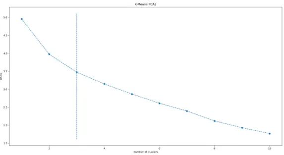
K-means clustering and spectral clustering algorithms require the number of clusters to be predefined before clustering. The elbow method was used to determine the optimal number of clusters for k-means clustering. Schlice proposed 6 clusters for this problem [2]. K-means elbow method shows that 3 clusters are optimal for this data set (figure 4.2). However, the elbow method
Figure 4.2: Elbow method showing 3 clusters.
is not reliable in this case as it produced a curve with a very small variance in the slope between the points. The number of clusters can be extracted from other clustering algorithms that can cluster and identify the number of clusters from data without being explicitly provided this information. Several experiments were conducted to cluster the data into three clusters as proposed by the elbow method and six clusters as proposed by Schlice. Grouped and ungrouped data sets were clustered and analyzed to identify what playstyles are expressed in those clusters and how they differ from each other. Increasing the number of clusters can result in over fitting where the model effectively learns where the points are in the given data set and would fail to cluster previously unseen data points. This can result in the model outputting several clusters where there is only one data point in the entire cluster [38]. Another sign of over fitting can be seen when the algorithm fails to assign a cluster label to some of the data points.
4.4
Chapter Summary
This chapter employed the data preparation methods that were described in 2.3. The data was normalized and PCA was applied to select only the most important features. The original data set containing 198 284 entries and 49 features were reduced to 24 races and 15 components. This chapter also identified 3 clusters present in the data set.
Chapter 5
Method
This chapter describes the experiment that was conducted during this study. It explains why this method of study was chosen and how it was carried out. This chapter also presents the measurements for the experiment.
5.1
Motivation
Computer science is closely related and is based on mathematics and logic [39]. Due to the nature of the research questions, theoretical approaches can-not answer them with confidence. A literature review or theory formulation cannot answer these research questions simply because scientific literature regarding RQ1, RQ2, and RQ3 does not exist. It is possible to extrapolate some general answers for RQ4 from already existing literature however this leaves RQ1, RQ2, and RQ3 unanswered. Furthermore, the validity of the answer to RQ4 would be questionable at best.
Adopting an engineering framework for the research allows for experimen-tation methods to be implemented. Experimenexperimen-tation eliminates the risk of subjectivity in the results and yields quantitative answers for the research questions [40]. Classification according to class intervals deals with numeri-cal data therefore quantitative study is preferable. Quantitative answers are desired in this study which attempts to improve an already existing model based on the previous studies as well as contribute to the computer science
field. Furthermore, the experiments allow for replicability and a controlled environment meaning that results should be the same every time the exper-iment is replicated [41].
5.2
The Experiment
The goal of the classification in this study is to extract the number of clusters in the data set and analyze them to identify the differences between them. Several experiments were carried out over the course of this study. Research question 1 is a meta-question and the answer for it is deducted from an-swering the RQ2. Anan-swering RQ2 required implementing multiple clustering algorithms to obtain their outputs for comparison and analysis. The cluster-ing algorithms were treated as independent variables and the clusters, and their assignments were held as dependent variables. The clustering perfor-mance was measured using the silhouette approach that is described in the next section as well as analyzing the individual clusters.
Implementation and testing of multiple classification algorithms were re-quired to obtain answers for RQ3 and RQ4. Classification prior to clustering was required for RQ3. It compared the clustering performance before the clustering labels were applied and after. The two outputs were compared in terms of accuracy. RQ4 was built on RQ3 where the initial classifications were the basis for comparison to which additional classification performances with reduced feature sets were compared. As a standard in the industry, the classifier performance was tested using 10 - fold cross-validation to prevent optimistic results and reduce bias [42].
5.3
Measurements
Measuring the performance of clustering algorithms and classification models requires established methods that would provide quantitative results.
5.3.1
Clustering Performance Measurement
Performance measurement of clustering algorithms can be obtained with the use of The silhouette method. Based on the dissimilarity matrix, the silhou-ette index provides insight into how well or bad the data is clustered. This method calculates the average distance between the data points in the cluster and the relation between the data within the cluster and all other clusters. [43, 44]. The measurement is calculated by the following formula:
s(x) = b(x) − a(x) max(a(x), b(x))
Where for each point x average distance between other points in its cluster is calculated and denoted as a(x) and b(x) denotes the smallest average dis-tance between the point x and the points in other clusters. This produces the silhouette index s(x) ∈ [−1, 1]. An index above 0.7 shows really good clustering results, 0.5 to 0.7 shows reasonable and confident clustering while results 0.2 and below should be interpreted as a lack of any significant clus-tering [45].
Silhouette index yields better results with centroid based clustering algo-rithms. The calculation of Euclidean distance between the points indirectly creates the center of the clusters. The silhouette index also yields better results when the clusters are similar in size. Measuring the distance between the points when the size of clusters differs drastically might provide inaccu-rate results due to a small cluster being relatively close to the center of a large cluster.
Silhouette index is not a hard rule, but rather an indication of clustering performance. Clustering performance is relative and has to be interpreted in the context of specific data set. The lack of ground truth in clustering per-formance prevents the creation of universal measuring methods. This thesis used the silhouette index as it measures the internal validity of clusters. Different measuring methods could have been used, however, it should not have a significant impact on the results. The silhouette index was measured across multiple clustering algorithms and the result was interpreted within the context of this particular data set.
5.3.2
Classification Performance Measurement
Classification performance can be measured by calculating the classification accuracy by the following formula:
a = c t
Where a is accuracy, c is the number of correct classifications and t is the number of total classifications. The amount of correct classifications is the sum of true positives and true negatives produced by the classifier model. Total classifications is the sum of true positives, true negatives, false positives, and false negatives. Accuracy will provide information on how well each model performs. Confusion matrices are presented to grasp the full context of the results. As an industry standard, the classifications were tested using 10 - fold cross validation. The data set is divided into 10 equal parts. One part is being used for training the model while the remaining data set is used as a testing set. This test is iterated until all parts are used as a training set [46].
5.4
Algorithms
Python scikit library was used in this research for the algorithm implementa-tion [47]. The library is being actively developed and is a common choice for data scientists. It contains machine learning and data preprocessing tools. Clustering attempts to find similarities between given data, therefore unsu-pervised machine learning algorithms were used. The selected algorithms dif-fer in their implementation and mathematical background. The list includes centroid based, affinity based and density-based algorithms. The choice of the algorithms is diverse and might provide completely different results. One specific approach might fail to cluster the data with confidence, therefore other approaches were included. The table below lists clustering algorithms that were tested in this study along with the section in this paper that de-scribes them (table 5.1). Classifications were performed using supervised
Table 5.1: Clustering algorithms that are tested in this study. Algorithm Section K- means 2.2.2 Hierarchical clustering 2.2.3 Affinity propagation 2.2.4 Spectral Clustering 2.2.5 Mean Shift 2.2.6 DBSCAN and OPTICS 2.2.7
machine learning algorithms as the purpose of the classification is to match given data with the correct label. This thesis used support vector machine (SVM) and logistic regression as those two algorithms were consistently pro-viding good results in A. Gustafsson’s study [1]. Additionally, the Gaussian Naive Bayes classification algorithm was used for the sake of comparison. The classifications were performed with raw data to obtain the base results for the classifications and then repeated with cluster labels. The results were compared to identify the effect the cluster labels have regarding classifica-tions.
To tackle research question 4, the classifications were performed multiple times. The data set was classified using a reduced list of features. Features were discarded one by one from the original data set and the reduced data set was classified, then classification was repeated with the cluster labels added to observe the difference. The data was clustered using 34 attributes as explained in section 4.2 which suggests that the classification would have to be performed for each possible permutation of the feature set. This high number of classifications restricts the use of Support Vector Classifier (SVC) which performed reasonably well in A. Gustafsson’s study. SVC operates in cubic time complexity O(n3) [48] and takes roughly an hour to train and
classify the data set using the hardware that is available for this research. A high number of permutations for the data set and cubic time complexity of SVC make it not possible to classify the permutation of 34 different at-tributes. To reduce the number of classifications required, the correlation co-efficient between features was extracted. The classifications were performed
only for the permutations where features involved have the highest correla-tion coefficient to cluster labels obtained through classificacorrela-tion.
The experiment was carried out using logistic regression, and SVC with linear kernel, which performed reasonably well in the related study, and naive Bayes classifier which has a time complexity of O(n) for the sake of comparison.
5.5
Chapter Summary
This chapter described the experiments that were carried out during this study alongside the motivation for this research method. The measurements for each experiment are defined. List of algorithms tested in this study are presented. The proposed experiment is to cluster the data using 8 different clustering algorithms. Identify the clusters from the results and add the cluster labels to the data set. Then use 3 different classification algorithms to predict the winner of matches. The classification has to be done using the original data set and the data set with cluster labels. Then measure the difference in accuracy.
Chapter 6
Results
This chapter presents the results obtained by conducting the experiments. The first sub-chapter displays the clustering results for selected algorithms. The second sub-chapter presents the classification results that were obtained with cluster labels obtained through clustering algorithms.
6.1
Clustering Results
The clustering was performed using 8 different algorithms. Hierarchical clus-tering is included to provide the dendrogram for the grouped data. Clusclus-tering non grouped data using hierarchical clustering was not feasible due to the implementation of the algorithm. BIRCH clustering algorithm is the imple-mentation of hierarchical clustering with optimization for large amounts of data, therefore this algorithm is included twice. The data was clustered us-ing 15 principal components, however, the figures below present the results plotted using two principal components that account for the most variance. Data was also plotted using three dimensions, however, it had no effect on the presentation or analysis of the results. Full-size images of the clustering results are available in the appendix 9.4.
6.1.1
Hierarchical Clustering Results
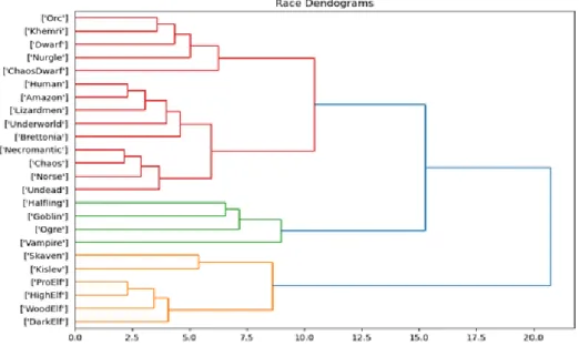
Hierarchical clustering identified three clusters (figure 6.1). The algorithms grouped all elven races together on one side of the spectrum, meanwhile, the bashier races such as undead and orcs were clustered on the other side of the spectrum in a different cluster. The third cluster that was identified consists of fairly few races, namely halfling, ogre, goblin, and vampires. This group was clustered roughly in between the other two clusters. As seen in the figure, his cluster is more closely related to the large, bashyer cluster than to the elegant elve cluster.
Figure 6.1: Race dendrograms displaying three clusters obtained trough hi-erarchical clustering.
6.1.2
K- Means Clustering Results
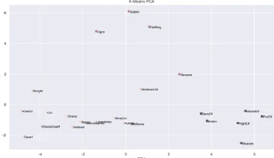
K- means clustering algorithms presents three clusters with a grouped data set that are identical to the results obtained with Hierarchical clustering (figure 6.2). In the figure, it is visible that the clusters are mostly spread
Figure 6.2: K-Means Clustering results.
out on one axis while, the middle cluster containing ogres, goblins, vampires and halflings are further away in a different axis.
Although all the data points are clustered and clusters are clearly separated, the silhouette index is relatively low due to the Vampire data point being closer to Underworld than to the cluster it belongs to (figure 6.3).
Figure 6.3: K- means Silhouette index.
6.1.3
Affinity Propagation Results
Affinity Propagation clustering grouped the data in the identical fashion as K-means and Hierarchical clustering (figure 6.4). This means that the silhouette index is identical to the k-means silhouette index (figure 6.5).
Figure 6.4: Affinity propagation clustering results.
6.1.4
BIRCH Clustering Results
BIRCH clustering is based on hierarchical clustering therefore the clustering results (figure 6.6) are identical to hierarchical clustering, k-means clustering and affinity propagation clustering. Silhouette index is identical to the pre-viously presented results as the clustering results were identical too (figure 6.7).
Figure 6.7: Silhouette index for BIRCH clustering.
6.1.5
Spectral Clustering Results
Spectral clustering yielded similar results to previous clustering algorithms, however it included Ogre in a large cluster and matched Amazon, Humans, and Lizardmen closer to Goblin and Vampires than to Norse and Bretonia (figure 6.8). Silhouette index shows all three clusters more similar in size than in previous clustering results, however, the silhouette index is signifi-cantly lower due to the small distance between clusters (figure 6.9).
Figure 6.8: Spectral clustering results.
6.1.6
DBSCAN Clustering Results
DBSCAN clustering failed to cluster some of the data points. The blue data points in the graph are not clustered (figure 6.10). This is reflected in the silhouette graph with cluster number 3 being empty (figure 6.11). The silhouette index is naturally lower due to unassigned data points around the clusters.
Figure 6.11: Silhouette index for DBSCAN clustering.
6.1.7
OPTICS Clustering Results
Similar to the DBSCAN clustering, OPTICS failed to cluster some of the data points that are colored blue in the figure below (figure 6.12). The Silhouette index shows that three clusters were identified, however, the fourth cluster is the ungrouped data points (figure 6.13). Silhouette index is 0 because the clusters and unassigned data points are overlapping.
Figure 6.12: OPTICS clustering results.
6.1.8
Gaussian Clustering Results
Gaussian clustering failed to cluster three data points and grouped Dwarves and Chaos Dwarves into a separate cluster (figure 6.14). Silhouette index shows two small clusters and one cluster that is empty and should have been the unclustered data points (figure 6.15).
Figure 6.15: Silhouette index for Gaussian clustering.
6.1.9
Mean Shift Clustering Results
This clustering algorithm clustered most of the data similarly to k-means and hierarchical clustering, however, it assigned Ogres, Goblins, Vampires, and Halflings to their own individual groups (figure 6.16). Silhouette index displays this over fitting problem (figure 6.17) where four clusters contain only one data point.
Figure 6.16: Mean Shift clustering results.
6.1.10
Summary of Clustering Results
Below is the table summarizing the clustering results for each algorithm. K-means, affinity propagation, and BIRCH have clustered the data identically and have the highest silhouette index. Gaussian clustering, OPTICS, and DBSCAN have the lowest silhouette index due to poor clustering and failure to cluster all the data points.
Algorithm Number of clusters Smallest Cluster Silhouette index
K- means 3 4 0.3586 Affinity Propagation 3 4 0.3586 BIRCH 3 4 0.3586 DBSCAN 2 4 0.2459 Mean Shift 6 1 0.2988 OPTICS 3 3 -0.0038 Spectral Clustering 2 6 0.1994 Gaussian Clustering 4 3 0.2316
Table 6.1: Overview of clustering results
6.2
Classification Results
Classification to predict the winner of the matches was performed using three different classification algorithms. These algorithms are SVC with linear kernel, logistic regression, and Gaussian naive Bayes. The following features were excluded from the classification data set as they were deemed to be a clear indication of the score:
GameWon Touchdowns
TouchdownsAgainst Score
The Classification was first performed without cluster labels to establish the base results to which other classifications would be compared. The classifica-tions were verified using a 10-fold-cross-validation. The classificaclassifica-tions were repeated with cluster labels (Segment) present. The results classification are presented in the table 6.2.
Algorithm Base Accuracy Accuracy with Segment Gaussian NB 0.765 +/- 0.005 0.761 +/- 0.004
Logistic Regression 0.898 +/- 0.003 0.902 +/- 0.003 SVC 0.899 +/- 0.004 0.900 +/- 0.003
Table 6.2: Classification results.
The confusion matrices are presented below in tables 6.3 for Gaussian naive Bayes classification algorithm, 6.4 for logistic regression algorithm and 6.5 for support vector classifier. The tables include the base results without the clustering labels in column ”Base” and the results with cluster labels present in column ”With segment”. This allows for a quick comparison of how the cluster labels affected the classifications. Interestingly, the confusion matri-ces show a slight increase in false positives when cluster label is introduced.
Actual
Base With Segment Positive Negative Positive Negative
Predicted Positive 36075 14398 35835 15147 Negative 13866 56135 13997 55495
Table 6.3: Gaussian Naive Bayes Confusion matrix
Actual
Base With Segment Positive Negative Positive Negative Predicted Positive 42801 5170 42852 5460
Negative 7160 65343 6954 65208
Actual
Base With Segment Positive Negative Positive Negative Predicted Positive 41822 4064 42197 4362
Negative 8186 66402 7638 66277
Table 6.5: SVC Confusion matrix
Python sklearn library allows us to extract feature weights for most clus-tering algorithms including SVC and logistic regression. These weights show how much each feature affects the outcome of the classification. Logistic regression and SVC use a variable threshold that allows to rank features according to the corresponding coefficient. Gaussian naive Bayes algorithm does not provide such functionality as the algorithm implementation does not rely on feature ranking, however, the feature weights can be calculated by employing feature permutation and measuring the difference in the outcome. Table 6.6 displays the feature weights for classification algorithms tested in this study. The weights were scaled using min-max scalar for readability and are not the actual weights used by the algorithms as the weights and the implementation of the algorithms are different.
The table displays that the SVC and logistic regression rank the features similarly while Gaussian NB ranks them completely differently. According to the table, the experience points are by far the most important feature in determining the outcome of the match while the race is the least rele-vant across all three algorithms. Furthermore, the heat-map depicting the Pearson correlation coefficient, shows that the segment is closely related to experience (0.58), breaks, blocks (0.69 for both), meters run (0.63), stuns (0.56), and knockouts (0.52). Classifying the data set with segment feature present and the features it correlates to omitted allows to compare the dif-ference in accuracy. Table 6.7 shows the results for substituting each of the mentioned features with cluster labels.
Feature SVC Logistic Regression Gaussian Naive Bayes Race 0.068023 0.097284 0.042095 KillsAgainst 0.197254 0.456784 6.344338 StunsAgainst 0.293975 0.179266 8.262674 CatchesFailed 0.619824 0.246158 0.412933 DodgesFailed 0.768945 1.510512 6.322288 Kills 0.770147 0.110210 1.872231 Pickups 0.911335 1.596677 0.158358 BreaksAgainst 1.878335 2.622739 15.316616 Dodges 1.922690 3.119459 0.394892 Knockouts 2.022859 2.026123 3.461824 KnockoutsAgainst 2.083281 3.339422 10.223104 BlocksAgainst 2.196318 2.542293 12.608495 PickupsFailed 2.375505 2.929630 2.670034 GFIs 3.039869 5.171728 5.502436 CasualtiesAgainst 3.289851 4.683917 15.779662 Turnovers 4.051758 6.312184 32.485417 Blocks 4.115322 5.405809 0.948143 Passes 4.268929 4.341638 0.627418 MetersRun 4.335602 2.694524 13.071542 Stuns 5.366657 4.687985 2.720148 MetersPassed 6.104048 6.877504 0.362820 Catches 7.138681 9.446147 0.388879 Sacks 7.519332 9.331611 2.585844 BallPossession 8.583984 9.479125 1.645719 Interceptions 9.008651 8.748704 4.307735 Breaks 9.938955 9.904657 6.406479 Completions 12.543312 12.726480 0.673522 Casualties 44.138440 43.574422 5.819151 XP 100.000000 100.000000 100.000000
Configuration Gaussian NB Logistic Re-gression
SVC
Base Accuracy 0.765 +/- 0.005 0.898 +/- 0.003 0.899 +/- 0.004 Accuracy with
Seg-ment
0.761 +/- 0.004 0.902 +/- 0.003 0.900 +/- 0.003
without XP 0.712 +/- 0.005 0.768 +/- 0.005 0.762 +/- 0.004 without XP and
Seg-ment
0.705 +/- 0.006 0.763 +/- 0.004 0.759 +/- 0.004
without Breaks 0.771 +/- 0.003 0.900 +/- 0.003 0.902 +/- 0.003 without Breaks and
Segment
0.772 +/- 0.004 0.899 +/- 0.004 0.899 +/- 0.004
without Blocks 0.763 +/- 0.004 0.900 +/- 0.004 0.899 +/- 0.004 without Blocks and
Segment 0.765 +/- 0.004 0.899 +/- 0.004 0.899 +/- 0.004 without MetersRun 0.761 +/- 0.006 0.899 +/- 0.003 0.897 +/- 0.004 without MetersRun and Segment 0.760 +/- 0.003 0.897 +/- 0.003 0.895 +/- 0.003 without Stuns 0.761 +/- 0.004 0.901 +/- 0.003 0.900 +/- 0.003 without Stuns and
Seg-ment 0.768 +/- 0.005 0.899 +/- 0.003 0.899 +/- 0.002 without Knockouts 0.767 +/- 0.003 0.901 +/- 0.002 0.899 +/- 0.004 without Knockouts and Segment 0.770 +/- 0.003 0.900 +/- 0.002 0.899 +/- 0.003
without all but XP and Segment
0.767 +/- 0.004 0.897 +/- 0.003 0.891 +/- 0.004
without all but XP 0.766 +/- 0.005 0.897 +/- 0.004 0.894 +/- 0.002
6.3
Chapter Summary
This chapter presented the clustering results alongside the silhouette index for each clustering algorithm. K-means, affinity propagation clustering, and hierarchical clustering provided nearly identical results while DBSCAN and OPTICS failed to cluster the entire data set. Results from the most confi-dent clustering algorithms were included in the data set. The resulting data were classified using Gaussian naive Bayes, logistic regression, and SVC. The clustering results show a slight increase in false positives and a decrease in false negatives when the cluster labels are introduced. Feature weight was ex-tracted for the classification algorithms and features related to cluster labels were removed. The results show no significant change in the accuracy even when cluster labels and features closely correlated to them are completely removed.
Chapter 7
Analysis and Discussion
This chapter presents the analysis of the results and compares clusters to each other to identify how they differ and what playstyles emerge in those clusters. The chapter also investigates the significance of classification accuracy change when the cluster labels are introduced.
7.1
Clustering Analysis
Hierarchical clustering, k-means, affinity propagation, BIRCH, and spectral clustering algorithms identify three distinct clusters. Two major clusters and one small cluster that is less prevalent and change the included data points depending on the clustering algorithm, however, it contains mostly the same races. It is safe to state that the data contains three clusters that are iden-tically grouped by four different algorithms.
Further data analysis supports the game community claims that the three clusters can be identified as Bash, Dash, and Hybrid. The clusters are num-bered automatically by the clustering algorithms. The numbers are 0, 1, and 2. The rest of this section will identify the differences between the clusters. The cluster 0 in this case can be called bash, it is the largest of the clusters. Races in this cluster have a high number of blocks, breaks, and casualties. Average number of passes in this cluster is 0 (figure 7.1).
Figure 7.1: Box plot showing passes for each cluster.
Cluster number 1 in the data can be called the hybrid. This cluster contains just four races: goblins, halflings, ogres, and vampires. Races in this cluster have a high amount of stuns, breaks, and knockouts which shows the similarities to the bash cluster, however, this cluster also shows a high amount of dodges and a low number of blocks which is more similar to the third cluster. The most interesting feature in this cluster is the lower number of touchdowns compared to the other two clusters and The higher score against it. It is worth noting that this cluster has less experience than the other two clusters (figure 7.2) which can explain lower numbers of touchdowns and higher scores against these races.
Cluster number 2 is the dash cluster. This cluster contains dark, high, wood, and pro elves as well as skaven as kislev. These races show low numbers in all of the aggressive moves such as blocks, knockouts, and stuns, but a very high number of passes, meters run dodges, and pickups.
Figure 7.2: Experience statistics for each cluster.
7.2
Generalization
Clustering was performed on the data set that was grouped by race. The grouping was done using median values. Clustering the data that is not grouped, provides similar results in terms of features and the difference be-tween clusters, however, each race is present in multiple clusters simultane-ously. Each race does not fall into a strict category of the playstyle, but rather has a tendency to lean towards it. The variations during each match results in a large spread of the features across each race. The figure 7.3 displays the variation in break actions for each race. It is clearly visible that there is a significant overlap between most races. The figure shows that the elves, kislev, and skaven have fewer break actions than the other races however the higher end of the distribution overlaps with the lower end of the vampires and dwarves who tend to have the most break actions. These Gaussian distributions can be observed in the rest of the features across the data set which further supports the claim that races do not fall into strict playstyle categories but rather lean towards it.
Figure 7.3: Breaks for each race.
Clustering not grouped data set into six clusters as proposed by Shclice [2] provided the same three clusters as outlined in the previous section however the clustering algorithms split the clusters by their experience level into the low experience and high experience clusters, even when the experience was not included in the clustering. Cluster number 1 (hybrid cluster), however, was split into one with a high luck rate and one with a low luck rate meanwhile experience in both clusters was identical. As mentioned in the previous section the hybrid cluster has a lower level of experience than the other