A Model-Driven Approach for modeling Heterogeneous Embedded Systems

(1)

Västerås, Sweden

Thesis for the Degree of Master of Science in Software Engineering - 120.0

credits

A MODEL-DRIVEN ENGINEERING

APPROACH FOR MODELING

HETEROGENEOUS EMBEDDED SYSTEMS

Vincenzo Stoico

vso18003@student.mdh.se

Examiner:

Jan Carlson

Mälardalen University, Västerås, Sweden

Supervisors: Federico Ciccozzi

Mälardalen University, Västerås, Sweden

Luigi Pomante

University of L’Aquila, L’Aquila, Italy

(2)

Abstract

Demands of high-performance systems guided the designers to the assessment of heterogeneous embedded systems (HES). Their complexity highlighted the need for methodologies and tools to ease their design. Model-Driven Engineering (MDE) can be crucial to facilitate the design of such a system. Research has demonstrated the usage of MDE to create platform-specific models (PSM). The aim of this work is to support HES design targeting platform-agnostic models. This work is based on a well-defined use case. It comprises a software application, written following the CUDA programming model, executing on a CPU-GPU hardware platform. The use case is analyzed to define the main characteristics of a HES. These concerns are included in a UML profile used to capture all the features of a HES. The profile is built as an extension of MARTE modeling language. Finally, the Alf action language is applied to make the model executable. The results prove the suitability of MARTE and Alf to create executable HES models. Additional research is needed to further investigate the HES domain. Finally, it is necessary to prove the validity of the UML profile targeting different programming models and hardware platforms.

(3)

List of Figures

1 Four Layers of Model Driven Architecture [26] . . . 9

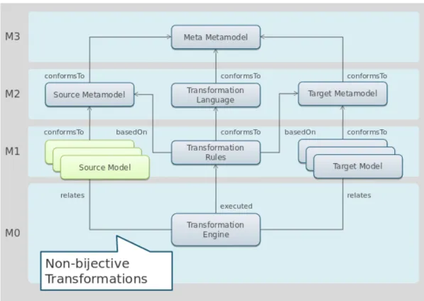
2 Non-bijective transformation in MDE stack . . . 10

3 Relational database metamodel . . . 10

4 Simplified UML metamodel . . . 11

5 Result of the transformation . . . 12

6 Class Overview . . . 13

7 Bidirectional Relationship Example . . . 14

8 Association Notations Overview . . . 14

9 Aggregation and Composition notations . . . 14

10 Interface PageSearch . . . 15

11 Actions Overview . . . 16

12 Flow Final Node . . . 17

13 ControlNodes Overview . . . 17

14 User authentication procedure . . . 18

15 Expansion Region with two inputs and one output [5, p.484] . . . 19

16 Application of the stereotype computer [30] . . . 19

17 Profile Diagram Overview [30] . . . 20

18 MARTE package architecture [6, p.13] . . . 21

19 The MARTE::CoreElements package [6, p.21] . . . 21

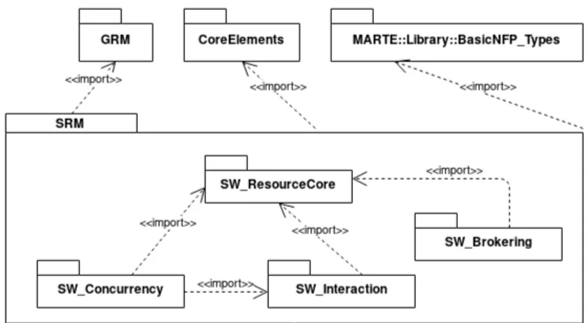
20 The Software Resource Modeling package structure . . . 24

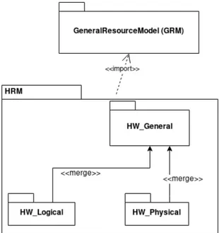
21 Hardware Resource Modeling structure (HRM) . . . 25

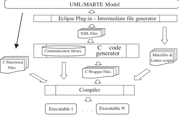
22 eSSYN execution flow . . . 28

23 Thesis Workflow . . . 31

24 Execution flow for a single character . . . 33

25 Use Case execution platform [31] . . . 35

26 Representation of the software application classes . . . 37

27 Structure of SystemDevice class . . . 38

28 Representation of the hardware platform classes . . . 39

29 First level organization of the NVIDIA GeForce 8800 . . . 41

30 Texture/Processor cluster (TPC) organization . . . 41

31 Streaming Multiprocessor Organization. . . 42

32 Concurrent Concatenation Activity Diagram . . . 43

33 Overview of the HESApplication package . . . 47

34 Overview of the HESPlatform package . . . 49

35 Overview of the HESCore package . . . 50

36 Software Application classes improved with the proposed stereotypes . . . 52

37 Hardware Platform classes improved with the proposed stereotypes . . . 53

38 First level of the NvidiaGeForce8800 structure improved with the proposed stereo-types . . . 54

39 Third level of the NvidiaGeForce8800 structure improved with the proposed stereotypes . . . 54

40 Classes representing virtual memory spaces . . . 55

41 Compiled representation of the WriteLine operation . . . 56

(5)

(6)

1. Introduction LIST OF FIGURES

1 Introduction

Nowadays, the presence of embedded systems in everyday life is tremendously grown. They are ubiquitous, most of the devices involved in our daily activities are based on an embedded system: consumer electronics, home appliances, cars. Usually, they are designed to perform a single function and are composed of a mixture of hardware and software. The design of embedded systems involves different metrics that must be optimized to create a product suitable for a given application domain. A design metric is a measurable characteristic of system implementation and its design process. Examples of design metrics are NRE cost (nonrecurring engineering cost), size, performance, time-to-market, correctness. An expanded list of common design metrics can be found in [1, pag.5]. These metrics impact on one another, so the aim of the design phase becomes to build an implementation that reflects an optimal trade-off among the design metrics. For this reason, the architecture of such systems can vary a lot according to the application domain. They may be composed by a heterogeneous set of hardware components: CPUs, GPUs, memories and a network of local connections among them, often on the same integrated circuit (i.e. System on Chip). This seems to be the best solution to reach positive results in terms of performance and flexibility. However, due to their complexity, the adopted design methodology plays a crucial role in settling the quality of the product.

A Model-Driven Engineering (MDE) approach can be useful to positively address design metrics. A model can be defined as an abstraction of the system-of-interest and accurately represents its essential characteristics [2]. The model is built according to a set of concerns (e.g. reliability, performance, concurrency) significant for several stakeholders (e.g. system users, system owners, developers). In this way, system properties can be easily analyzed and its behavior can be predicted. Section2.1 discusses the MDE context. OMG proposed different languages and profiles to solve questions related to the embedded system context. Examples are SysML, UML Profile for Schedulability, Performance and Time (SPT), UML-RT, UML profile for the Modeling and Analysis of Real-Time and Embedded systems (MARTE). The latter seems to be the most suitable language for modeling of real-time embedded systems. Several models can be used to highlight different characteristics of the system-of-interest. Each one can be seen as a view of the system. Models can be manipulated to ensure consistency among the views. This feature is called model transformation. Model transformations can be classified as Model-to-Model (M2M), Model-to-Text (M2T), Text-Model-to-Model (T2M) transformations [11, pag. 107]. Thanks to M2T, the code can be automatically generated from one or multiple source models. In the context of the embedded systems, this can be crucial for system verification. Indeed, for hardware engineers, it can be useful to automatically generate a simulator of the underlying platform. This is a powerful mechanism to obtain a better result in reducing development time and costs and improving code quality and maintainability.

The adoption of heterogeneous embedded systems (HES) comes with further pros and cons compared with those of a single-core architecture. The former comes with a broader range of hardware combinations. For example, a HES can be composed of: CPU + GPU, CPU + FPGA, CPU + DSP. So, additional considerations should be made during the modeling phase. One of the main advantages of such a system is that the workload can be divided between the available Processing Units (PU). However, to exploit the benefits of the underlying platform, the application should be written following parallel programming models 1. This increases the complexity for a programmer. For example, a programmer may deal with data dependencies between processes or deadlock states. This kind of properties can be checked statically on the model. Other issues may result from the characteristics of the platform. For example, software execution can be affected by the available CPU-GPU memory bandwidth, memories size, PUs capacities. These problems can also be addressed during the design phase.

1

"A parallel programming model describes an abstract parallel machine by its basic operations, such as arith-metic operations, spawning of tasks, reading from and writing to shared memory or sending and receiving mes-sages." [12]

(7)

This work moves towards a solution to support the designer during the development of a heterogeneous embedded system. The solution proposed focuses on the efficient usage of model-driven engineering practices to address the problems coming from the HES domain. This thesis looks for a methodology capable for modeling of both hardware and software characteristics. Due their complexity, it is crucial the exploration of techniques for the verification of developed artifacts. This work comes up with procedures to prove system correctness. So, the scope of this thesis includes the investigation of practices of model simulation. Section 2 widely discuss the background needed to understand the content of the research. Section 3 describes previous works done in this field. Instead, Section 4 presents an analysis of the context in which this work takes place. Furthermore, it presents the questions investigated during the research. The methodology used to develop the research is presented in Section5. Section6shows the adopted solution. The application of results is discussed in Section 7. Finally, the obtained results are examined in Section 8.

(8)

2. Background Model-Driven Engineering

2 Background

This section presents a deep discussion of the concepts needed to understand the context and the proposed solution. Firstly, Section 2.1describes the Model-Driven Engineering (MDE) domain. In general, the MDE paradigm uses system models to guide the design process. The research is carried out following the directives of languages and tools adopted in the MDE domain. Then, Section2.2outlines the Unified Modeling Language (UML). It is one of the most used language for the creation of models. This subsection discusses the UML elements involved in the research. Finally, Section 2.3 reports the MARTE language. It extends UML including system features not covered by the semantics of UML. For example, MARTE elements may have information to report real-time features.

2.1 Model-Driven Engineering

Modeling is a cognitive process focused on the generation of an artifact used to represent the real world. It is a very common practice, it is performed by people in everyday life for communication purposes. Indeed, it provides an abstraction of the real world that does not capture it as a whole, but that highlights its specific characteristics. The usage of models is wide-spread and their usefulness is evident in various contexts. Architecture is one of the fields that gets more benefits from modeling. In this field, is usual to have scale models representing physical buildings that are not still realized. These are needed to make evidence of the building design decisions. Physicians use equations as mathematical models to represents properties of real world objects. For instance, with the following formula it is possible to express the frequency of a pendulum: f = 2πq_Lg [21]. It is well-known that, in the engineering domain, the development of complex systems implies the employment of modeling techniques. In particular, software systems can take considerable advantages from modeling since they may be exceptionally complex. The development process involves the participation of several stakeholders. The stakeholders class incorporates all those entities contemplating the system. Examples of stakeholders are companies, designers, customers. A stakeholder is interested in one or more concerns affecting the system. A concern can be defined as a concept that has an influence on the system and its environment. So, examples of concerns are performance, structure, behavior, maintainability, usage, security. A set of concerns can be seen as a viewpoint and they are realized in a view that highlights them. For instance, a state chart diagram is usually used to describe the interaction (i.e. the behavior) of different part of the system. Follows that multiple views of the system can be created to describe different aspects of it. This is particularly useful when stakeholders comes from distinct domains. The meaning given to the concept of view converges to the definition of model.

A good model is built keeping into account a precise and clearly defined purpose. Examples of purposes are: requirements description, simulation, verification of timing constraints. Model-ing purposes can be classified in two categories: descriptive purposes and prescriptive purposes. In the first category are placed all those models that are less detailed. They are usually used for communication like describing the system to the stakeholders and to emphasize specific system characteristics. Instead, the second category is needed to represent all those models that are quite detailed and used to predict system features. Martin Fowler proposes a further distinction, targeting UML [5] models, specifying three categories called UML Modes 2_{. However, this}

dis-tinction applies even for the general practice of modeling. He categorizes models in three classes: models as sketches, models as blueprints, models as programming languages. The former cate-gory includes all the models used for communication purposes. Sketches are adopted to discuss, with the team, about some aspects of the system like issues in the code or alternative paths. They cannot be usually found in system specifications since they are informal and quickly done. Blueprints are detailed model used by the programmers as guideline to write the code. These

2

(9)

models can be found in software documentation and are usually done by a senior programmer that gives them to the developers. They are created using tools designed for modeling like Com-puter Aided Software Engineering (CASE) tools. Finally, blueprints should contain all design decisions and should strictly respect system requirements. Models can be detailed enough to substitute programming languages. The main reason to follow this way is productivity. More-over, models should include semantics to enable their execution. These kind of models can be also used to generate the application code. For Fowler, this is not true3 since modeling practices are based on a set of standards (e.g. UML, MOF, XMI) that together can be seen as a platform. A software development process that employs models as first-class objects is commonly referred as Model-Driven Engineering (MDE). MDE can be seen as an alternative approach to handle system development in which are expressed guidelines for system modeling.

A model is created following the rules of a modeling language. The latter enables the definition of a tangible representation of the system. It is possible to express a language with a clearly established notation. The meaning of each notation element is specified relating them to a semantic domain. The language notation is also called concrete syntax and it defines how the language should appear [22, p.143]. The concrete syntax is important for language understandability and expressiveness. Furthermore, there are many concerns that should be taken into account to evaluate a good concrete syntax: writability, readability, learnability, effectiveness [24]. The notation may be textual, graphical or both. A language can have many concrete syntaxes depending on what you want to represent. For example, these are three different notation to express the same concept: 2 + 3, (+23), (23+) respectively called infix, prefix, postfix. In the abstract syntax is specified the semantics of the language. It includes all the concept names and their relationships [22, p.143]. The set of rules characterizing elements relationships is also known as structural semantics. The last one is usually expressed in ad-hoc constraint language like Object Constraint Language (OCL) or in natural language. One way to define an abstract syntax, for a natural language, is through the creation of a grammar written in Backus–Naur form (BNF). A BNF is a notation for context-free grammars in which are defined symbols and rules to compose the sentences. It enables the generation of all possible language sentences. The following is an example of a context-free grammar taken from [23].

<noun-phrase> -> <cmplx-noun> | <cmplx-noun><prep-phrase> <verb-phrase> -> <cmplx-verb> | <cmplx-verb><prep-phrase> <prep-phrase> -> <prep><cmplx-noun>

<cmplx-noun> -> <article><noun>

<cmplx-verb> -> <verb> | <verb> <noun-phrase> <article> -> a | the

<noun> -> boy | girl | flower <verb> -> touches | likes | sees <prep> -> with

The sentences below can be obtained from the above grammar:

the boy sees a flower

a girl with a flower likes the boy a boy sees

As shown in the previous paragraph, models are used for different purposes. Depending on it, it is clear that models can be differentiated according to their accuracy. A modeling language may contain syntax to describe, in detail, domain aspects or they can be general

3

(10)

Model-Driven Engineering

leading to less accurate models. All those languages conforming to the first definition are labeled as domain-specific modeling languages (DSL) while those in the second one general-purpose modeling languages (GPML). A typical GPML includes abstractions to allow the description of several concepts coming from multiple domains. So, it comes with a great number of elements. An example of GMPL is UML [5]. On the other hand, a DSL is built with a fewer number of elements since it describe a specific application domain. Examples of DSLs are those languages needed for description like Hypertext Markup Language (HTML) or hardware description languages (e.g. VHDL or Verilog).

Once clarified the concepts related to a language, a model can be seen as an abstraction of the reality conforming to the abstract syntax of a modeling language and represented by one or more concrete syntaxes. The abstract syntax can be treated as a model as well and takes the name of metamodel. This name suggests the idea of something that is at a higher level of abstraction. This denomination is contained in the framework proposed by the Object Management Group (OMG). OMG is a standards consortium that presented many languages and tools to ease the adoption of such a paradigm [25]. The OMG called this vision of MDE as Model Driven Architecture and relies on the adoption of OMG standards. A metamodel, in turn, is described using a meta meta model, so a more abstract language that defines the semantics of a metamodel. The big picture of this hierarchy is captured by a stack that has at its top a language built using its own semantics: the Meta Object Facility (MOF) language. MOF is a ad-hoc language for metamodels design [9]. The [27] gives to MDA the denomination of technical space. The work defines a technical space as "model management framework containing concepts, tools, mechanisms, techniques, languages and formalisms associated to a particular technology.". Another example of technical space is the one from the W3C consortium that promotes XML as a language for the definition of metametamodels. Fig.1 is a graphical representation of the languages stack taken from the [26, p.250]. The image depicts the stack defined for the UML language. As can be seen, the UML metamodel (i.e. level M2) is an instance of the MOF language. Consecutively, the model at M1 conforms to the semantics defined at M2. In this case, M2 can be extended through the definition of stereotypes. This metaclass characterization is implemented annotating it with the label «stereotype». This mechanism is elaborated in Section

2.2. Finally, at the bottom of the stack (i.e. level M0) there is the real processor, so the physical object in the real world.

One of the most important ingredients of MDE is model transformation. The term trans-formation refers to a mapping procedure between elements of two models. As for modeling languages, model transformations require a language for the creation of rules to be applied upon models. The mapping is done at metamodel level and then applied as a template to their in-stances. The source and target models involved in the transformation can conform to the same metamodel or to a different one. In the former case, the transformation is called endogenous while in the second case exogenous. The [27] proposes a definition of model transformation as a non-bijective function that associates multiple source models to several target model. This degree of generality includes a transformation from one source model to one target model or from a single source generating multiple targets. Fig.2represents a non-bijective model transformation along with the abstraction layers for the definition of modeling languages. Moreover, a transformation can be executed in the other way, so from a target model to a source model. If a transformation can be performed in both ways then it is called bidirectional otherwise unidirectional. Another classification can be done keeping into account the objective of the transformation. For example, a transformation from a more abstract model to a more concrete one or the other way around. This application is commonly called vertical transformation. Code generation and reverse engi-neering practices are labelled as vertical transformations. Instead, if the transformation generates two models at the same abstraction level is called horizontal. Examples of the last one are view consistency management and change propagation. This is relevant when the stakeholders come from different domains since it allows the creation of several models described with different

(11)

Figure 1: Four Layers of Model Driven Architecture [26]

languages.

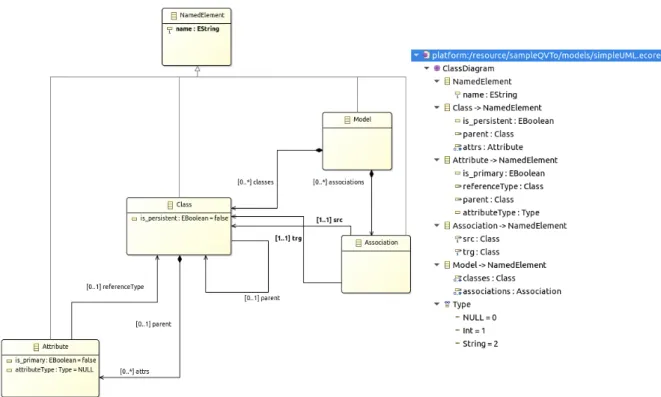
OMG consortium includes in the MDA technical space a standard for the creation of modeling languages named Query/View/Transformation (QVT) [28]. QVT specification is composed of a declarative part that includes two languages: QVT Relations and QVT Core. The QVT Relations language comprises notation and semantics for the definition of mapping between model elements in a declarative fashion. For example, it formalizes one of the building block for a mapping that is the concept of relation. Indeed, a relation is a construct used to define constraints that must be verified in both models. Finally, it allows the automatic generation of the transformation trace and provides semantics to define bidirectional transformations. QVT Core contains semantics for the concepts defined in the QVT Relations language. It is simpler and describes only the mapping between model elements. However, the transformation trace must be explicitly specified. The declarative part is enriched with the possibility to use transformations in a procedural way. QVT incorporates OCL extensions that enable the transformations realization following the imperative paradigm. These are contained in the language called QVTOperational. The following example, is an application of QVTOperational using two metamodels. The source model conforms to a simplified version of the UML metamodel. Instead, the target metamodel contains concepts from the relational database (RDB) domain. The objective is to automatically obtain a database schema from a class diagram. This transformation can be realized using the QVTOperational implementation added to the Eclipse Modeling Framework (EMF) [29]. Fig.3

and Fig.4 represent, respectively, the rational database metamodel and the uml one. The left hand side shows a graphical version of the metamodel using the UML notation, while the right hand side its tree based version.

4_{taken from the slides: "Model Transformations: an introduction" of Prof. A. Pierantonio for the MDE course} at University of L’Aquila

(12)

Model-Driven Engineering

Figure 2: Non-bijective transformation in MDE stack4

(13)

Figure 4: Simplified UML metamodel

The source model is an instance of the simplified UML metamodel and describes a library. The library consists of the classes: Book, Member, Librarian, Transaction and their relationships. The Transaction class exemplifies the loan of a book. Listing1is the code used for the transformation.

Listing 1: UML to RDB transformation code

1 modeltype UML uses’http://www.xeder.org/simpleUML’; 2 modeltype RDB uses’http://www.xeder.org/rdbms’; 3

4 transformation SimpleUML2RDB(in uml : UML, out RDB); 5 6 main() 7 { 8 uml.rootObjects()[UML::Model]−>map model2RDBModel(); 9 } 10

11 mapping UML::Model::model2RDBModel() : Rdbms::Schema 12 {

13 name := self.name;

14 tables := self.classes−>map class2RDBMTable(); 15 }

16

17 mapping UML::Class::class2RDBMTable() : Rdbms::Table 18 {

19 name := self.name;

20 cols := self.attrs−>map attr2RDBMColumn(); 21 }

22

23 mapping UML::Attribute::attr2RDBMColumn() : Rdbms::Column 24 {

25 name := self.name; 26 }

The first two lines are needed to specify the source and the target metamodels. The addresses on these lines are the Uniform Resource Identifiers (URI) of the metamodels. They are used to uniquely reference the metamodels. The statement at the line four is the transformation

(14)

Unified Modeling Language (UML)

signature. It specifies the names of the input and output models. The main() block is the first one to be executed. It can be seen as a list of rules consecutively executed. The statement at the line eight is called entry operation and it invokes the first mapping. The mapping between the remaining elements will be executed recursively according to the reference established in the model. Indeed, at the top-level, it is called model2RDBModel() that implements the mapping between the concepts of model and schema. The block model2RDBModel() executes, in turn, class2RDBMTable() that calls another block. This mechanism is applied for all the elements involved in the operation. A block is declared using the keyword mapping along with the name of the source model, the mapping name and the return type. Listing 2 describes the structure of a mapping block.

Listing 2: Mapping block structure

1 mapping<context_classifier>::<mapping_name> ( <parameters> ) : <return_type> 2 {

3 <mapping body> 4 }

Fig.5 depicts the result of the above described transformation. The left hand side is the source model while the right hand side the resultant.

Figure 5: Result of the transformation

2.2 Unified Modeling Language (UML)

The Unified Modeling Language (UML) is a visual modeling language used for analysis, design and implementation of a system. UML is a general-purpose language, so it is not bound to a specific domain. Furthermore, it is defined as a standard from the Object Management Group (OMG). It is composed of elements with simple semantics. This led the language to be spread used and adopted for different purposes. UML has feature to design both the structure and the behavior of a system. This is crucial for a designer that wants to evaluate system correctness. Its notation can be suitable for modeling of complex embedded systems. UML supports several Electronic System-Level (ESL)5 design flows. For example, it can be appropriate in a top-down design or in a hardware/software co-design. However, since it is a general purpose, it may lack

5_{"the utilization of appropriate abstractions in order to increase comprehension about a system, and to enhance} the probability of a successful implementation of functionality in a cost-effective manner." [4]

(15)

syntax and semantics for specific domains. A real-time embedded system can require additional timing information, to check schedulability or to perform timed simulations. UML is able to fill this absence through the usage of profiles [5, pag.252]. This section describes three of the diagrams contained in UML. Section2.2.1analyzes the class diagram necessary to figure out the system structure. Instead, Section 2.2.2concerns one of the diagram used for system behavioral description: the Activity Diagram. Finally, Section 2.2.3 illustrates the profile mechanism and the related diagram to represent it.

2.2.1 Class Diagram

A class diagram is used for structural modeling of a target system by means of classes and interfaces. In particular, it is focused on classes characteristics, constraints and relationships. The Class concept conforms to the homonym one from the object-oriented paradigm. It is a classifier [5, p.99] acting as an abstraction for entities with common structure and semantics. A class is capable to encapsulate a composite internal structure and to present a behavior. The first mentioned comprises all the features referring to the instances structure. This kind of features is also known as structural features. For example, a class property is a structural feature. Instead, the behavioral aspects are captured by the concept of behavioral feature. The latter includes class operations. In the graphical representation of a class, these are usually divided in compartments as shown in Fig.6. A class can be defined also as an abstract class. It is a class that can’t be directly instantiated and it is needed only for other classes to inherit features from it. When a class is abstract, its name is written in italic.

Figure 6: Class representation [30]

A class property could delineate a class attribute, the member end of a relationship and a part of a structured classifier. Generally, an attribute comes with its type, multiplicity and name. However, it may hold several additional properties that are known as slots. An example may be an attribute of type Patient that holds the slots: id, name and gender. UML enables the designer to specify the visibility of its features. If a feature is public it will be visible to all the elements in the same namespace [5, 27]. The public visibility is identifiable with the addition symbol (i.e. +) applied to the target feature. The private one obliges the element to be visible only in the namespace that owns it (e.g. the same class). A private element is represented by the - literal. A protected element is visible to elements possessing a generalization relationship to the namespace that includes it. The placeholder that stands for a protected element is the # literal. Finally, UML can bind an element to the closest enclosing package. Outside this package, the element is not visible. The symbol standing for a package visibility is the ˜ symbol. Class properties can be constrained using a constraint language as the Object Constraint Language (OCL) [33]. Class instances are commonly called objects. An object is usually rendered with a name and its type underlined. Diagrams containing only objects are called object diagrams and are considered instances of class diagrams. They show the specification of class values and object relationships.

The relationships between classes are expressed with the usage of associations. Associations are employed to simply relate classes or to combine them in aggregates. In fact, an association can be binary when involves two classes (i.e. bidirectional) or n-ary when concerns at least three classes. In the last case, it is shaped as a diamond. Instead, a bidirectional association is drawn

(16)

as a solid line. The aspects of an association are indicated at its ends. At both ends may be placed a role name and a multiplicity value.

Figure 7: Bidirectional Relationship Example

Fig.7 shows the relationship between a Flight and a particular Plane. If the association is read from the point of view of the Flight, then it means that when an instance of a Flight exists, it can either have one Plane associated with it or no one. If the association is read in the other direction, then it means that plane can be assigned to zero or more flights. The navigability of an associations is an important property too. An association is navigable when at least one of its end can easily access instances of the other end at run-time [5, p.200]. An association end has different notations to express unspecified navigability, the navigability direction or the non navigability. Fig.8 shows the usable notations.

Figure 8: Association Notations Overview

The association (1) has unspecified navigability at both ends while, in the (2), the Flight class has unspecified navigability and the Plane one is navigable from Flight. Finally, the as-sociation (3). As introduced above, asas-sociations have also the capability to model grouping of class instances. For this purpose, an association may be a aggregation or a composition. They are both used to show that a class A is composite of a group of instances of a class B. An aggregation is a binary association that indicates a "weak" relationship between the composite class and the one that makes it up. This means that if an instance of the composite class ceases to exist then its component is still available to be used. Instead, a composition is a form of "strong" relationship in which if the composite is deleted, then all of its parts are deleted with it. Fig.9 depicts the notation for the aggregation and the composition. The former is drawn as an association with an hollow diamond while the latter with a filled black diamond.

Figure 9: Aggregation and Composition notations

Finally, an association can point out a vertical relationship among two classes. This means a relationship between a more abstract class and its specification. This kind of association is called generalization and it is drawn as a line with a hollow arrow at the end of the general classifier. Other than classes, a class diagram can present interfaces. An interface includes attributes

(17)

and operations that must be provided by the class realizing the interface. It can be seen as a contract. However, interfaces are not instantiable and they serve just as a specification for the classes implementing them. An interface is graphically marked with the keyword interface. The relationship between a class implementing the interface properties and the interface is called interface realization dependency and it is drawn as a circle. Instead, the correlation between the class using the interface properties (i.e. class that requires the interface) and the interface is named usage dependency. The notation for a usage dependency is a half-circle. Fig.10illustrates the interface PageSearch and how it is provided/realized by the classes.

Figure 10: Interface PageSearch

A class diagram can specify also data types [5, p.167]. A data type is a classifier whose instances "are distinguished only by their value". A data type supports attributes and operations to model structured data types. They can be assigned to an attribute of a class. They are equated to a C structure or a Java Class. A data type is characterized by the keyword «dataType» on its top.

2.2.2 Activity Diagram

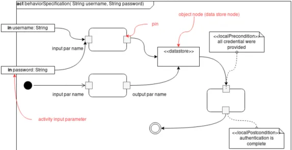
An Activity Diagram is used to describe a flow of actions, giving prominence to the conditions leading to their execution. An Activity is the crucial element of this diagram and it is represented as a graph. The graph nodes are instances of the metaclass ActivityNode connected by ingoing and outgoing edges conforming to ActivityEdge metaclass. A node is needed to describe the backbones of a behavior: the required actions and the involved objects while the edges their execution order. A node can assume three different connotations: control nodes, object nodes and executable nodes. The executable nodes are those representing a single step of the graph. They are labeled as executable since they can be processed by an execution engine [5, p.441]. An execution engine is required to evaluate the nodes under different point of views. It can optimize the execution of the activity to satisfy certain extra functional requirements. For example, an engine can be set to run an activity step of step or to change the flow of execution according to a common characteristic (e.g. how much they interact). However, during the engine execution, it is not possible to violate the UML specification. An executable node gives the possibility to connect several exception handler to it. An exception handler can be used to model anomalies during the execution of the flow. All the types of executable nodes are specialization of the metaclass Action. An action is executed atomically and cannot be further decomposed. An action can be constrained by a precondition and a postcondition that must be held respectively before and after the execution. An action is said to be opaque when a different concrete syntax, other than the UML one, can be used to write its specification. The semantics of an opaque action cannot be interpreted since UML specification does not provide any mechanism to check it. An action is represented with a rounded square and, eventually, with attached pins to show consumed inputs and produced outputs. A pin wraps the definition of a parameter that are its type and multiplicity. Fig.11 shows an activity with preconditions with connected pins.The multiplicity can be expressed as a single value or as an interval. The multiplicity value on an input pin leads the action to not start its execution if the number of presented inputs is less than the specified value or interval lower bound. The same thing applies for an output pin: an action cannot terminate its execution until the number of consumed outputs is the same as the

(18)

Figure 11: Input parameters, Pins and Object nodes graphical representation

multiplicity value or interval lower bound. When an action is triggered for other meanings other than the execution flow, its inputs can be calculated as described in the owned pins of type: ValuePin and ActionInputPin. The former enables the evaluation of a ValueSpecification whom result is used as input to the action who wants to execute. An action input pin provides the input to an action calling another action. The last one is indicated in the fromActions attribute of the ActionInputPin. To build higher level models or structured actions, UML contains Call Behavior actions and Call Operation actions. A Call Behavior action can be bound with whatever instance of the Behavior metaclass (e.g. an activity). Instead, a call operation action can be mapped to an instance of the Operation class [5, p.116] to describe its behavior. The object nodes are used to describe the object flows. Under the UML language viewpoint, an object node is an instance of a classifier and together with object edges are used to define data dependencies. The semantics of object nodes is captured by the ObjectNode metaclass. In the diagram, an ObjectNode is needed to show that a classifier instance will be obtainable at a certain step of the flow. They are depicted using rectangles. The already described Pin class, is an instance of the ObjectNode metaclass. Other commonly used ObjectNode specializations are: central buffer, activity parameters and data store node. Input and output parameters are passed to an activity execution applying the ActivityParameterNode metaclass. An ActivityParameterNode should correspond to each parameter with direction in, out, inout or return direction [5, p.147]. These ones are part of the ParameterDirectionKind. The in literal is employed for input that may not be modified during the execution. The out literal is used for parameters passed to the caller. The return one for the return value of the call. Finally, the inout literal points out an input parameter that is altered during the execution and then passed to the caller. A central buffer node works as a buffer between the ingoing and outgoing edges. Instead, a data store node permanently stores flow objects. When a object is requested, it is placed on the outgoing edge. However, its copy remains in the buffer for subsequent requests. Fig.11 presents the data store object node and two activity input parameters.

The control nodes are those needed to coordinate several ActivityNodes. They come with distinct types: initial node, flow final node, activity final node, decision node, merge node, fork node, join node. Fig.13 is an overview of control nodes. The initial node designates the starting point of an activity. An activity can have more initial nodes, it means that flow starts from multiple sources. A decision node has been introduced to implement conditionals in the diagram. It represents the situation in which a single outgoing path is chosen from one or more incoming path. The choice is performed according to a condition expressed by a label (i.e. guard). The adopted symbol is a diamond-shaped box. It has the same semantics of a

(19)

switch-Figure 12: Flow Final Node

case statement when it presents more than two outgoing edges. A merge node is depicted with the same symbol of the decision node. However, it is needed to redirect more incoming path in a single outgoing path. The reader can recognize a merge node when the diamond presents several incoming paths e one outgoing path. Furthermore, it can be found an hybrid solution in which the decision and the merge node can be combined together leading to a diamond showing multiple incoming paths and many outgoing paths with an attached condition. An Activity Diagram has the capabilities to model the concurrency of multiple flows. This is done using a fork and a join node. A fork node divides one flow in multiple streams that are equal. The opposite is done by the join node that is used for the synchronization of the concurrent flows. It presents several incoming edges and a single outgoing. The join node can present a condition to be satisfied for the synchronization. The condition is indicated in curly brackets located above the symbol. The meaning of the default guard is the equivalent of an AND logic port. The join and the fork node can be merged in a single statement as done for the decision/merge node. A flow is ended using the final nodes. A flow final node terminates the flow. It terminates all the flows reaching the flow final node. However, the activity is not terminated if there are remaining executing flows. Fig.12 represents the symbol of a flow final node. Instead, a activity final node specifies the termination of all the flows involved in the diagram. It is shown in Figure13.

Figure 13: ControlNodes Overview [30]

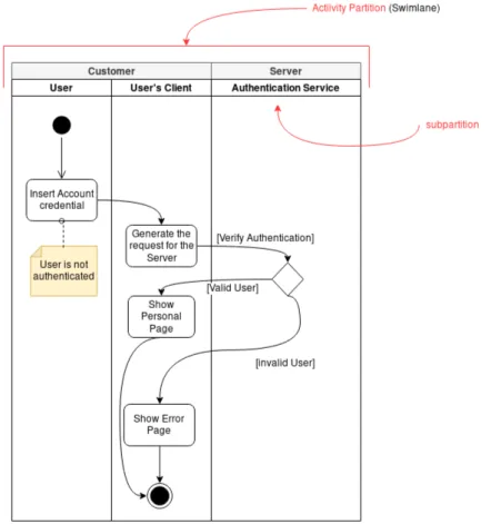
The edges that permit the transfer of object between ObjectNodes are occurrences of the ObjectFlow metaclass. An ObjectFlow instance can have an associated behavior required to modify the passing object. This kind of behavior has an input parameter and an output one. It comes in two flavours: as a transformation or a selection. A selection obliges the input parameter to be unordered, nonunique and with multiplicity of 0..*. Instead, the output parameter must have its multiplicity upper bound set to 1. A transformation enables to have several instances of the output parameter as an output. An ObjectFlow can have set both the transformation and the selection behaviors. In this case, the transformation one is firstly executed. A notable feature of an Activity Diagram are the Activity partitions. Activity partitions are used to group the actions according to common characteristics. For example, it is possible to categorize the occurrences of a classifier through an activity partition. Common usages of partition involve classifiers, properties and instance specifications. The graphical notation representing a partition is the swimlane one. Each lane contains the behavior responsible for the instances of a given classifier, property or InstanceSpecification [5, p.140]. A partition can be composed by subpartitions specifying the attribute isDimension = true. For instance, a partition can have a dimension to specify the location of an action and another one to perform

(20)

Figure 14: User authentication procedure

it. Finally, a lane can be external. The scope of an external partition is to create conscious exceptions to the normal usage of a partition. For example, it is possible to show the structure of a classifier. An external partition is noticeable if the «external» label is present and the attribute isExternal is true. Fig.14 shows an activity diagram representing the authentication procedure of a user.

An expansion region is a kind of structured node that figures out actions that are repeated for a collection of input values. In case of a behavior that produces outputs, these can be accumulated in an output collection. The eventual input and output collections are graphically specified as a collection of pins placed at the boundaries of the node. These are commonly known as expansion nodes. Inside an expansion region, there is the description of the behavior for a single element of the input collection. The region is executed once for each element of the collection. When several input expansion nodes are present, then the number of executions is the same as the size of the smallest input collection. The way in which the execution is conducted is expressed by the mode attribute that may have the following values:

• When the value of the mode attribute is parallel the execution engine process the values of an input expansion node concurrently.

• The inputs can be evaluated iteratively. In this case, the behavior in the expansion region is applied one for each element of the input expansion node. The expansion region works as a for loop.

• If the mode attribute value is stream, then the elements contained in the collection flow in the region as a single execution.

(21)

Figure 15: Expansion Region with two inputs and one output [5, p.484]

2.2.3 Profile Diagram

A profile diagram is the representation of how the UML semantics can be extended. A profile is commonly defined as a lightweight extension of the UML metamodel. The word "lightweight" is particularly suitable to define a profile since, the latter, does not change (i.e. strong change) the UML structure, and extends it with the introduction of classes targeting specific domains. So, profiles can be seen as specific types of packages recognized by their uri. An instance of an uri can be seen in Fig.17. The extending classes are visually identifiable since they have the label «stereotype» on their top. Instead, a metaclass coming from the UML superstructure, is marked with the keyword «metaclass». A stereotype can have its own attributes called tag definitions. When a tag is applied to a model (i.e. Fig.22), including its actual value, it is named tagged value. Fig.16shows the application of the stereotype «Computer» for the modeling of a particular computer. When a stereotype is applied, the resulting class, is displayed with the name of the stereotype enclosed in double-angle brackets.

Figure 16: Application of the stereotype computer [30]

The extension of a metaclass can be expressed by a filled arrow as shown in Fig.17. An extension is a kind of association and it is navigable from the end of the stereotype. Instead, for the metaclass, the extension is treated as an owned property [30]. An extension can be marked with the required label to indicate that an instance of the stereotype is obliged to be connected to an occurrence of the metaclass. A profile can be imported into other packages using dependency relationships. To show that a package has been applied to another package the «apply» stereotype can be assigned to a directed relationship. This is shown in Fig.17. Multiple profiles can be applied to a package if there aren’t conflicts between each other. Finally, for deeply structured profiles, it may be useful to use the «reference» keyword on a directed relationship. It is needed to identify the reference metamodel elements that are imported in a separate package. Furthermore, filtering rules can be applied. This rules are required to figure out which elements are visible and which ones are hidden when the profile is applied.

(22)

MARTE

Figure 17: Profile Diagram Overview [30]

2.3 MARTE

MARTE stands for Modeling and Analysis of Real-Time Embedded Systems and it has been created with the aim to complete the already existing profile called UML for Schedulability, Performance, Time. MARTE has been conceived to address two operations performed during system design: modeling and analysis. Indeed, it allows the design of both hardware and software components independently. The profile is structured to model the system at different levels of abstraction. So, it is possible to describe the system in general terms or build very detailed models. This choice is influenced by the scope of the design. For example, code generation usually needs very detailed models. MARTE architecture is represented in Fig.18. This section deeply explains all the modeling features of the profile. The analysis section is fundamental for modeling of embedded systems but it is out of the scope of this work. Section2.3.1discusses two sub-packages adopted for modeling behavior and data types: CoreElements and NFP. Section

2.3.2 presents the GRM package. It is the sub-package including elements for modeling a generic resource and its related services. Finally, Section 2.3.4 and 2.3.5 reviews the SRM and GRM sub-packages. They needed to model, respectively, hardware and software resources.

2.3.1 MARTE Foundations

At the top level, there is the Foundations package. It is the most abstract package and it includes the basic concepts of the language. A striking example of this is its sub-package: CoreElements. It permits to distinguish between classifiers (e.g. Class, Interface) and their instances. This divergence is critical for modeling and analysis purposes. Moreover, this feature is not included in UML. Fig.19 shows the shape of CoreElements. As presented in the picture, it provides the basic elements to express the behavior of the system-of-interest. Particular attention should be paid on the CommonBehavior sub-package. Indeed, it defines the semantics for the concepts of Behavior, Event and Trigger. These concerns are important for the description of more elaborated ones. For example, the Event and Trigger stereotypes are referenced in the Time sub-package. It can be used to model the activation of an event, after a prefixed duration.

(23)

Figure 18: MARTE package architecture [6, p.13]

(24)

MARTE

Properties of a system can be categorized in functional and non-functional ones (NFPs). The first type concerns all the services that are provided by the system, instead the second one all the constraints applied to the system. It includes timing constraints, constraints on the development process or resource utilization constraints [3]. This category is of particular interest, since its influence contributes to several design decisions. This necessity is even more clear when it comes to constrained systems. The MARTE NFP sub-package supplies semantics to represent NFPs and to attach them to a UML model. The NFP package is structured in 3 sub-packages: NFP_Nature, NFP_Declaration, and NFP_Annotation. NFP_Nature defines the distinction between a quantitative property and a qualitative one. A quantitative property is a quantifiable aspect of the system. It can be measured at run-time during a simulation. Instances of quantitative property are the throughput or the latency. This kind of property can be modeled as metrics expressed with the class Quantity according to a reference Unit. The units that may be used are worldwide accepted and established in the International System of Units 6. Moreover, it is connected to the concepts of sample and measure. The first one refers to a set of values that can occur during the measurement of a quantitative property. Instead, a measure is a function that is applied to the sample to discover some its characteristics. These concepts are described by the homonyms classes. A quantitative property is different since it is not quantifiable. It refers to an abstract description of a general property relevant for the analysis. A qualitative property is often implemented through labeling. An example can be the label assigned to a task to indicate its priority. So, the semantics included in this package is needed to produce a description of property characteristics. The NFP_Declaration sub-package defines an abstraction of a NFP property that is called value property. It is the representation of a general physical quantity. A value property is modeled using the ValueType class. The latter is a specialization of TupleType that is a combination of several data types in a single entity. The ValueType stereotype provides two attribute: valueAttribute and expAttribute. The first one is the resulting value obtained from the expAttribute expression. These concepts are needed to state the structure of the property. The NFP_Annotation permits to define extension points to an existing model. Indeed, it defines the class AnnotatedModel composed of several AnnotatedElement instances. For example, they may be used to describe some kind of analysis implementing as annotated elements: a step (i.e. a unit of execution), scenario (sequence of steps), resource and services [6, p.40]. Moreover, the annotated element permits to link model elements to system non-functional properties. For example, it is possible to model the time spent executing a step or the utilization of a resource.

2.3.2 General Resource Modeling (GRM)

The General Resource Modeling (GRM) package is part of the top-level components of MARTE. It includes general concepts including semantics for system analysis and detailed modeling. These concepts are further specialized in the sub-packages: design model and analysis model. GRM is built around the notion of resource. It is generally defined to represent an entity coming both from software and hardware domain. A first example of this feature may be a clock that can be both physical or logical. The difference is that the time elapsed on the second clock can be counted also using processor cycles rather than common time metrics. A resource can perform services to satisfy functional or non-functional requirements. GRM permits to lower the level of abstraction instantiating the resource concept with several stereotypes. The resource concepts is specialized in the stereotypes: SynchronizationResource, ConcurrencyResource, ProcessingResource, StorageResource. The SynchronizationResource is used to manage the access to shared re-sources. This is the general metaclass that is detailed by the classes referring to scheduling. The ConcurrencyResource defines resources capable to perform its flow of execution simulta-neously with other resources. The ProcessingResource stereotype identifies a resource capable

6

(25)

to execute schedulable resources. It comes with a generalization needed to represent an external device, a communication resource or a scheduler. An external device can be modeled using the DeviceResource stereotype. Instead, a communication resource concept is mapped with the CommunicationMedia stereotype. A communication media may be seen as an end point involved in the communication process. This connotation is captured by the CommunicationEndPoint stereotype. The StorageResource is adopted to include memories in the model. A scheduler is defined as an entity capable to manage run-time behavior. In particular, it has access to pro-cessing resources and it is mapped by the homonym stereotype. A scheduler hosts zero or more schedulable resources. The latter are instances of ConcurrencyResource competing to control available resources. Resource services can be modeled too. The stereotype ResourceService allows the definition of services to allocate or deallocate a quantity (e.g. memory) from a given resource (e.g. storage). Finally, GRM, has notions to design resource management services. For example, the ResourceBroker is delegated to assign or deny resources to an entity that requested it. It enables the description of a control policy that defines the criteria for the allocation. The ResourceManager is another kind of service that is responsible of the life cycle of the resource. It creates, deletes and maintains a resource according to a given policy.

2.3.3 High Level Application Modeling (HLAM)

The high level application modeling (HLAM) package introduces the basic concepts to model constrained systems. It relies on the semantics described in the GRM, CoreElements and the GCM packages. The package is built around the RtUnit stereotype. It has the same purpose of an active object but it contains tags to model real-time applications. Indeed, the creation of its instances implies the execution of a real-time service. The latter is associated to a RtUnit through the tag main, and described through the operationalMode. This one has type Behavior and usually is a state based representation. Furthermore, the RtUnit stereotype, includes the tag queueSchedPolicy to manage concurrent incoming messages. The reception of a message can trigger the instance of a service. All the characteristics of a service are captured by the stereotype RtService. The transition of messages from a source to a target are shown by the RtSpecification stereotype. It enables the modeling of the messages arrival pattern through the homonym attribute. Furthermore, it is possible to specify priorities, deadlines, and general timing properties. The information shared between the concurrent flows are reported using the stereotype PpUnit, namely a protected passive unit. Finally, for each PpUnit, it can be specified the accessing policy and its memory footprint.

2.3.4 Software Resource Modeling (SRM)

The software resource modeling (SRM) [5, p.196] is a specialization of the GRM package. This package is needed to model software applications with a focus on concurrency, process synchro-nization, and hardware resource management (e.g. memory brokering).

The SRM package is composed of the following sub-packages:

• SW_ResourceCore provides the basic concepts for software modeling.

• SW_Concurrency allows the designer to include concurrent execution in its model.

• SW_Interaction provides semantics for modeling process synchronization

(26)

MARTE

Figure 20: The Software Resource Modeling package structure

The SW_ResourceCore sub-package provides the backbones of the SRM package. It includes the classes SwResource and SwAccessService. The first one identifies a generic software resource, it is a specialization of the class Resource contained in the GRM package. The SwResource [6, p.227] has attributes to specify the services to create, delete or start the resource on a target system. These features are mapped respectively with the attributes: createServices, deleteServices, initializeServices. Furthermore, the state and the occupied memory can be included with the attributes: stateElements and memorySizeFootprintElements. The SwAccessService serves to access SwResource characteristics. It as the same role of Java getters and setters. The SwAccessService is a specialization of the GRM ResourceService class.

The SW_Concurrency [6, p.200] defines the concepts needed to model parallel execution. Moreover, it defines semantics to incorporate all the resources needed by processes (e.g. registers, interrupts). The SW_Concurrency package is built around the concept of SWConcurrentResource. This class represents elements that may execute concurrently part of the application. It is a spe-cialization of the SwResource class contained in the SW_ResourceCore sub-package. It is associ-ated to an execution flow represented by the EntryPoint class. Indeed, the SwConcurrentResource contains the attribute entryPoints. It defines the attribute to describe the behavior to sus-pend, resume and terminate the concurrent resource. The attributes to do this are respectively: suspendServices, terminateServices, resumeServices. Furthermore, a concurrent resource can use portions of the heap and the stack. This feature is pointed out with the attributes heapSizeElements and stackSizeElements. Finally, the execution of a process can be confined within a virtual address space. The addressSpace attribute defines the address space used by the execution of concurrent resources.

An one or more address spaces belong to the memory partition. The latter is modeled with the MemoryPartition class contained in this sub-package. The relationship between the address spaces and a memory partition is expressed through the attribute memorySpaces. The SwConcurrentResource is a generalization of InterruptResource and SwSchedulableResource. Both of them propose semantics for process arbitration. The competition for shared resources can happen at physical level or at software one. The InterruptResource serves for scheduling at physical level. It offers services to manage an interrupt service routine (ISR). A SwSchedulableResource is a specialization of classes SwConcurrentResource and SchedulableResource. The last one can be found in the GRM package. It describes a software resource that can be associated to a scheduler that can handle its execution.

The SW_Interaction [6, p.202] sub-package contains the concepts to model synchronization between concurrent resources. The SwInteractionResource helps to model a waiting queue for resource preemption. It owns the attributes waitingQueuePolicy, and waitingQueueCapacity. They are needed to express, respectively, the queuing policy kind (e.g. FIFO, LIFO) and the capacity of the queue. Furthermore, it is possible to specify a waiting policy for a single ele-ment. The attribute waitingPolicyElements is used for this purpose and allows the following

(27)

Figure 21: Hardware Resource Modeling structure (HRM)

policies: ready, waiting, waiting with a time out, and conditional waiting. In this context, con-current processes need both to interact among themselves and to communicate data. So, the SwInteractionResource is specialized in two main classes: the SwCommunicationResource and the SwSynchronizationResource. The latter is used to synchronize mutual access to shared data (e.g. semaphore). Instead, to notify special conditions to waiting resources, it can be used the NotificationResource class. Instead, the SwCommunicationResource, is necessary to model artifacts for communication purposes (i.e. custom data types). It is instantiated in two classes: MessageComResource and SharedDataComResource. The second one allows a reference to a memory portion shared between concurrent resources.

The SW_Brokering [6, p.205] sub-package supplies semantics to manage hardware resources. It is composed by two classes: DeviceBroker and MemoryBroker. A DeviceBroker instance works as interface between the application and the peripheral devices. Instead, the MemoryBroker class manages the allocation, the mapping, and the protection of a memory.

2.3.5 Hardware Resource Modeling (HRM)

The Hardware Resource Modeling (HRM) [6, p.235] package is required for modeling of the hard-ware platform of an embedded system. The architecture of such a platform may be substantially dissimilar taken two different systems. For this reason, this package allows the definition of a generic model that can be used for several instances of an embedded system. It is a formal alternative to block diagrams. The structure of the HRM package is made by three packages: HW_General, HW_Logic, HW_Physical.

The HW_General includes the classes to define the structure of the execution platform. A generic hardware component is identified by the HW_Resource metaclass that is a specialization of the GRM Resource. It can be composed of other HW_Resource instances as it happens in a heterogeneous embedded system. A hardware resource is always bound to at least one service. This concept is addresses through the HW_ResourceService class. The latter is the specialization of the GRM ResourceService. The HW_ResourceService represents a service that a hardware resource can offer to another entity.

The hardware resource can be classified according to their functionality so, by the services that it offers. The HW_Logical sub-package includes computing, storage, communication, timing or device resources. The HW_Processor is one of the most important classes in this set and it is

(28)

MARTE

a hardware computing resource. It identifies a processor and it comes with plenty of attributes to specify its characteristics. For example, MIPS, instructions per cycle (IPC), number of cores, pipelines, and arithmetic logic units (ALU). Furthermore, MARTE allows the modeling of an instruction set architecture (ISA) instantiating the homonym class (i.e. HW_ISA class, and branch prediction (i.e. HW_BranchPredictor). All the computing resources of the HRM package are a specialization of the HW_ComputingResource metaclass. This package carries out the typical classification for the memories. Indeed, it includes the HW_Memory class that is the most abstract class denoting a memory. It could be an HW_ProcessingMemory or HW_StorageMemory. Volatile memories are modeled by the former including the technology whereby is built. For example, a cache is often built using an SRAM, while a RAM adopting an SDRAM due to its speediness. This two kinds of volatile memory are mapped respectively by the HW_Cache and the HW_RAM classes. The HW_StorageMemory is used for permanent storage modeling. It is further specialized in the metaclasses identifying a ROM (i.e. HW_ROM) and a mass storage memory (i.e. HW_Drive). The communication is a crucial aspect of a hardware platform that if often controlled through the adoption of structured protocols. The class representing the general concept of medium is the HW_Media that is further specialized in HW_Router, HW_Bus, and HW_Bridge. The HW_Router provides semantics to describe how data will be transmitted to the connected devices. For example, its attribute switchingType has literals for packet switching and circuit switching. Instead, the HW_Bus models a hardware bus. It comes with its address and word width. Finally, the masters connected to a medium need to be managed to take control of the medium. This job is done by an arbiter. The HW_Arbiter serves for this purpose. A bus master must be an instance of the HW_EndPoint class.

The HW_Physical [6, p.245] model categorizes the hardware components according to plat-form physical properties such as their shape, size, power consumption, size within the platplat-form. This is a fundamental aspect of an embedded system since usually, it comes with limited re-sources. The HW_Component has many attributes to specify construction characteristics. For example, for an HW_Component the designer can illustrate its dimensions, position, number of pins, price and weight. Many kind of components are available in this sub-package as the chip (i.e. an integrated circuit) , the hardware channel, the port, a unit (i.e. an identified area of an integrated circuit). A channel is a collection of wires used to connect the components.

(29)

3 State of the Art

Gaspard2 is a modeling environment for data-intensive application [14][15]. Its objective is to provide a tool suitable for modeling of both the application and the underlying platform. Gaspard2 is built upon MARTE profile and extends it with concepts needed to design embedded systems for data-intensive applications. The algorithms are described using the built-in repetitive structure modeling (RSM) package [6, p.529] that is used to model parallelism both for task and data. Instead, for hardware implementations, it is used the HW_Logical sub-package. It is needed to describe hardware components along with their extra-functional requirements. In this way, both the hardware and the software architecture are modeled independently. Finally, each software functionality is mapped on the desired hardware component through the Alloc package of MARTE. The latter is just used to map amounts of computations to processing units, so problems related to task schedulability are not taken into account by Gaspard2. The major extensions that Gaspard2 provides to MARTE are in favour of code generation. The first one includes additional semantics from a MoC based on Array Oriented Language (ArrayOL). ArrayOL is used to describe intensive multidimensional signal processing [16]. In this language, a task T is instantiated in multiple task instances. Each one takes a subset of the inputs of T. A subset is called pattern. The second extension is needed to include deployment information to the hardware and software component. It is crucial for code generation targeting different programming models and tools. In this way, it is possible to evaluate the design with different hardware and software configurations. The Gaspard2 project has been extended with a branch including support for OpenCL [18] as a programming model. The [19] describes an MDE-based approach to generate code for OpenCL applications. The approach concerns a chain of transformations composed of 9 steps. A UML model is given as input to the first piece of the chain and is augmented with low-level details transforming it according to the MARTE meta-model. Then, ArrayOL patterns are obtained and converted into repetitive tasks. The work utilizes a static scheduling policy to manage task execution that could not lead to optimal utilization of resources. Step 7 includes information about the allocation of each memory bank. The resulting model is close to the OpenCL specification and it is ready to be used to automatically generate the code. The code generation performed with Acceleo [20].

Intel proposes a modeling framework both for hardware and software of embedded systems called CoFluent [17]. The framework comes with an Eclipse-based tool that enables the simu-lation of a UML model built with a subset of SysML and MARTE. Furthermore, it includes an additional UML profile that extends the semantics of SysML [10] and MARTE profiles [6]. In particular, predefined model elements (e.g. divider, clock generator, message routing function), C/C++ code statements (e.g. directives, variables, type definitions) and design parameters cru-cial to simulate the model in different conditions. The elements of CoFluent are organized in the model packaging that is useful to provide differentiation between the software model and the hardware one. Moreover, it contains a package Allocation needed to map the application elements to the platform ones. CoFluent inherits the feature of MARTE of designing both the application and the platform in two different views. Once mapped, the resulting model is a vir-tual system since it embraces both system hardware and software characteristics. Finally, Intel implemented a Model-To-Model (M2M) transformation between a SysML/MARTE application model and the Intel CoFluent model. The resulting model conforms both to the latter and the ECore meta-model. The Ecore meta-model is included in the Eclipse Modeling Framework (EMF) [8]. The obtained model is used to generate a SystemC TLM [7] model that is needed to simulate the system.

(30)

3. State of the Art MARTE

Figure 22: eSSYN execution flow

The University of Cantabria proposed a framework called eSSYN in the Pharaon FP7 project. This framework includes solutions for the design of concurrent applications. The designer can specify hardware platform details and how to allocate software functions to hardware resources. The framework uses UML/MARTE as modeling language, both for the application and the platform. The user can describe the system using a platform-independent model (PIM). System functionalities are defined as an interconnected set of components and their communication as service calls. The components are defined using the «RtUnit» stereotype of MARTE. A component can assume the role of client or server according to the services that they require or provide. Services calls can be also chained. The communication between components can be seen as a service request. The characteristics of the latter and its parameters are specified in the interface shared between the components. Apart from the signature of the function, the interface specifies the run-time behavior of the call. It can be indicated, in the interface, using types defined in UML. Among them there are: sequential, guarded, concurrent. The guarded and concurrent properties are of particular interest since they permit to model the situation in which several invocations of a procedure can occur simultaneously multiple times. The parameters of service are specified as a custom data type. A client may send an amount of data that exceeds the capacity of the server. In this case, the call is divided into two invocations executed in parallel. Finally, the stereotype «RtUnit» includes the property «srtPoolSize» that permits the designer to define the number of threads that can be dynamically created. The framework allows to clearly model the differences between a service call and the way in which the underlying platform handles the request. A service call is managed through the use of a communication channel. The stereotype «CommunicationMedia» is used to define a communication channel. However, this stereotype, contains only properties related to the physical aspects of the communication. For example, it allows the definition of its capacity and mode (e.g. duplex) [5]. This work presents a little extension to include the run-time behavior of the client/server during a request (i.e. priority, blocking). The channels characteristics are captured with external components using the stereotype «ChannelTypeSpecification». Finally, the channel kind in use during a specific interaction is specified in the UML connectors involved in the interaction. ESSYN