Volatility forecasting in the Swedish hedge fund market : A comparison of downside-risk between Swedish hedge funds and the index S&P Europe 350

J

I

B

S

JÖNKÖPING UNIVERSIT Y

Vo l a t i l i ty f o r e c a s t i n g i n t h e Sw e

-d i sh h e-d g e f u n -d m a r ket

A comparison of downside-risk between Swedish hedge funds and the index

S&P Europe 350.

Subject: Bachelor’s thesis in Economics 2012 Author: DONALD HARDING, 1984-07-10 Tutor: Per-Olof Bjuggren, Professor

Louise Nordström, PhD candidate Jönköping May 2012

Bachelor’s thesis in Economics

Title: Volatility forecasting in the Swedish hedge fund market

Author: Donald Harding

Tutors: Per-Olof Bjuggren & Louise Nordström

Date: May 2012

Subject Terms: Hedge Funds, Value-at-Risk, VaR, FHS VaR, Expected Tail Loss, GARCH, EGARCH, ARMA.

Abstract

The purpose of this thesis is to examine whether Swedish Equity L/S hedge funds present a lower market risk than the index S&P Europe 350 over our holding period using a GARCH/EGARCH Value-at-Risk model. The sample consists of 96 monthly observa-tions between March 2004 and February 2012. The examination shows that the hedge funds in general hold a lower market risk than the index for the next holding period and al-so present a lower estimated loss if our VaR loss is exceeded. This implies that hedge funds would be a good choice for investors to have in a portfolio to reduce the risk.

Table of Contents

Abstract ... i

1

Introduction ... 1

1.1 Previous research ... 1

1.2 Purpose and problem discussion ... 4

1.3 Method... 4

1.4 Limitations ... 5

1.5 Structure ... 5

2

Theoretical framework ... 6

2.1 Hedge Funds ... 6

2.2 Standard & Poor Europe 350 index ... 8

2.3 Value-at-Risk ... 8

2.3.1 Historical and Filtered Historical Simulation of Value-at-Risk ... 9

3

Method ... 10

3.1 ARMA ... 10

3.2 GARCH models ... 11

3.3 Filtered Historical Simulation ... 13

3.4 Expected Tail Loss ... 13

4

Data ... 14

4.1 Description of data ... 14

4.2 Sample size and sources... 14

5

Empirics... 15

5.1 Hedge fund selection ... 15

5.2 Descriptive statistics ... 15

5.3 ARMA modeling ... 16

5.4 GARCH estimations ... 17

5.5 Filtered Historical Simulation of Value at Risk ... 18

5.6 Expected Tail Loss ... 19

5.7 Analysis ... 19

6

Conclusion ... 21

References ... 22

Appendix 1

... 1

1

Introduction

This section will introduce the subject and present an overview of previous studies performed within the field of hedge funds and Value-at-Risk measurements. It will also present the purpose and the problem discus-sion, a short overview of the method, limitations and what the reader can expect from the upcoming parts.

In times of financial crises and highly volatile markets the need for funds with comparative-ly small downside-risk has increased. The Swedish hedge fund market has shown a large in-crease in the number of registered hedge funds over the last years (Anderlind et al. 2003), from the first Swedish hedge fund introduced in 1996 until today when there are approxi-mately 70 active hedge funds in Sweden holding 5% of the total managed value of Swedish funds (Strömqvist, 2009). The increase in numbers of funds has made the new investment form more available to private investors than before. But what are the characteristics of this asset class, and more interesting how high/low is the downside-risk? Hedge funds have a reputation about themselves, most often self-possessed, to beat the index which is widely known. But there is little research about the downside-risk that an investment in a hedge fund holds.

When the hedge funds started using more complex financial securities such as derivatives,

collateralized debt obligations (CDOs) and other complex securities, it created problems with opacity and the need for risk management became more evident. Value-at-Risk (VaR) is today one of the most important and most used concepts for determining the total risk of a security or portfolio.

This study collects returns from five Swedish Equity Long/Short hedge funds and returns from S&P Europe 350. We will then calculate the historical VaR that an investment in ei-ther of these asset classes holds in order to determine if hedge funds provide a lower downside-risk than indexing. The VaR will be estimated as a percentage of the invested capital and calculated by using a generalized autoregressive conditional heteroscedasticity (GARCH) model to forecast the volatility for the next period. The GARCH-model first introduced by Bollerslev (1986) will allow us to use a conditional variance, which differenti-ates itself from the standard VaR-model by assuming a static variance. The results will then be compared and tested to see which investment model that holds the lowest downside-risk and if we can draw any conclusions about the best choice between hedge funds or the more passive investment strategy indexing.

1.1

Previous research

Much of the previous research performed on hedge funds has been focusing on the return side of the distribution. However, Brooks and Kat (2002) find that, even though hedge funds are assumed to carry lower risk than the average fund due to their strategies of

per-have a majority of net long exposures. This implies that the funds are significantly correlat-ed with the market and therefore also would carry the same risks as the market. Edwards (1999) claims the opposite, that the returns of hedge funds actually have low correlation to equity and bond returns. This is later confirmed by L’habitant (2004) who argues that due to the specifics of hedge funds such as equity-like returns and bond-like volatility, they are optimal to use in portfolios to move the efficient frontier to the northwest. This is due to the low correlation of bonds and equity to hedge funds, implying higher returns and lower risks.

Fung, Hsieh (2004) and Jaeger, Wagner (2005) find that for the equity hedge funds most of the managers prefer to go long in small cap stocks and short in large cap stocks. They argue that this might be because it is easier for the funds to find good investments in bull markets and it would also be easier to go short in large cap stocks due to the trade liquidity.

Edwards and Liew (1999) examine monthly returns from 1500 American hedge funds be-tween 1989 and 1998 and compared it to traditional asset classes such as equity and bonds. They find that the average return for hedge funds during this period was 14.23 % while S&P 500 equity index and long-term corporate bonds had average returns of 16.47 and 10.39% respectively. The comparison covers the summer of 1998, which according to Ed-wards (1999) include a period with substantial losses for the hedge fund industry, which forced many funds to shut down due to bad performance. Edwards and Liew further argue that when comparing the returns of surviving and non-surviving funds the commercially available figures of annual hedge fund returns might be inflated by as much as 1,9% by on-ly looking at surviving funds.

Gregoriou (2002) performs a survival analysis for hedge funds between 1990-2001 on the Zurich Capital Market database and found that the median life of hedge funds was 5.5 years. He also find that it exists common specifics among the surviving funds such as low minimum purchase requirements, size (large), low level of leverage and high returns. Brooks and Kat (2001) point out a problem with hedge funds and hedge fund indexes, which is the survivorship bias and find that as little as 30% of the newly introduced funds survive the first three years. Previous research on survivorship biases among hedge funds shows a quite large spread from 0.16% (Ackerman et al. 1999) to 3.0% reported by Fung and Hsieh (2000). Liang (2000) proposes a way to explain the differences by looking at the different databases used and their specific properties and also if they include fund of funds which tend to have a longer life than the average hedge fund. Moreover, Brown and Goetzmann (1995) and Brown et al. (2001) say that the survivorship would also have an impact on the degree of serial dependence in the return distribution, while Füss et al. (2006) state that the serial dependence comes from the infrequent trading in hedge funds. The hedge fund market in 1996, when the first Swedish hedge fund was introduced was mainly focusing on Global Macro funds according to Strömqvist (2008). But in later years there has been a shift of strategy towards Equity L/S funds and the Swedish hedge fund market has moved towards a strong bias in Equity L/S funds (Strömqvist, 2009).

Lo (2001) claims that even though risk management has a long track record he argues that the traditional way to analyze risk in hedge funds are not enough since they don’t capture the total risk that a hedge fund is exposed to. He introduces a new set of risk measure-ments, which contains the previously described survivorship bias. L’habitant (2001) on the other hand claims that the Value-at Risk is a result of the important development in calcu-lating financial risks and says that VaR is the “Best practices for assessing the total market risk exposure”. This is also confirmed by Pérignon and Smith (2006) who states that VaR is broadly used within in the financial sector.

The foundation of VaR as a risk measurement is J.P. Morgan’s document RiskMetrics from 1994 that present a set of techniques to measure the market risk in portfolios. They made their work public together with Reuters for three reasons (J.P. Morgan, 1996).

- Since the key to effective risk management is transparency, they wanted to promote a larger transparency in market risk measurements.

- To establish a standardized measurement for market risk. - To help their clients to measure their market risk exposure.

Many critics and opponents of VaR claim that the method is not sub-additive (Artzner et al.1997, 1999 and McNeil et al, 2005). They argue that VaR is not sub-additive, which means that the sum of two separate funds risks may be lower or equal to the total risk of the portfolio. The problem if risks are not sub-additive is that it goes against the idea of di-versification and fundamentals of modern portfolio theory, which is, without the sub-additivity there are no incentives for investors to hold portfolios. Daníelsson and Jorgensen (2005) argues that VaR on the other hand is sub-additive for most practical applications and that there is no reason to use more complicated risk measurements than VaR. We will due to the inconsistency use ETL as a complement to our VaR-measure since ETL is sub-additive (Szegö, 2004).

The symmetric normal GARCH model was developed by Bollerslev (1986), which is an ex-tension and a generalization of Engel’s (1982) ARCH model. Engel (1990) later proposed the A-GARCH model which capture the asymmetric parts in the returns inform of the lev-erage effect. The EGARCH model introduced by Nelson(1991) captures the levlev-erage effect but has the advantage that no restriction has to be imposed to ensure the non-negative condition for the conditional variance. We will use the asymmetric EGARCH model to-gether with the symmetric GARCH (p,q) in this paper to model volatility clustering.

Barone-Adesi et al. (1999) have developed the Filtered Historical Simulation (FHS) as an extension of the former volatility adjustment process thru volatility weighting first intro-duced by Duffie and Pan (1997). The idea of the FHS according to Baron-Adesi (1997) is to use a GARCH model, which is a parametric dynamic model of the returns volatility to create simulations of log returns over the risk horizon.

The FHS has met some critics and mainly from Pritsker (2001) who investigates both FHS and a variant of the Historical Simulation (HS) introduced by Boudoukh (1998). Pritsker

claims that both methods are under-responsive to the changes in conditional risk, he also says that the models reaction to risk is in an “asymmetric fashion”. Another main criticism in Pritskers paper is that he says, “FHS method requires additional modifications to ac-count for time-varying correlations and to choose the appropriate length of historical sam-ple period. Analysis indicates that two years of daily data may not contain enough extreme outliers to accurately compute VaR at a ten-day horizon using the FHS method”, Pritsker (2001). Although Pritsker presents some shortfalls of the FHS method for example Alex-ander (2008) argues that it has some distinct advantages over the Historical Simulation due to its ability of mixing Monte Carlo Simulation and Historical Simulation, which is the most frequently used method to calculate VaR among practitioners (Perignon and Smith, 2006).

1.2

Purpose and problem discussion

Previous studies within the field of hedge fund risk are mainly performed on the US hedge fund market and then also as Füss et al. (2006) on US hedge fund indexes. There is a low amount of research made on the Swedish hedge funds, which is why this paper will focus on Swedish Equity L/S Hedge funds and their ability to reduce the downside-risk.

The purpose of this thesis is to examine whether a sample of equity L/S hedge funds pre-sents a lower downside-risk then the passive form of investing known as indexing, and in this case we use the well-diversified index S&P Europe 350. We will try to see if an investor can obtain a lower VaR i.e. a lower exposure to market risk by choosing a hedge fund in-stead of a passive investment within an index.

1.3

Method

I have chosen historical VaR simulation since it is more commonly used among banks than the Monte Carlo and the parametric linear methodology according to Pérignon and Smith (2006). They found that 64.9% of the firms who unveiled their methodology, 73% used the historical simulation to estimate the VaR that their investments holds. VaR is usually used to predict short-term risk exposures, since data from long time-periods can bias the VaR estimate so that the models takes events into account that are unlikely to occur within the short time horizon for the VaR estimate. There is one exception to that rule according to Alexander (2008), who says that the simulation can be used for longer time horizons when the funds are locked in, which is the case for the monthly traded hedge funds that we will examine.

I will also conduct a Conditional VaR also called Expected Tail Loss (ETL), which is a measure of how much the investor can lose given that the initial VaR has been violated. The ETL is used as a complement to the historical VaR simulation because it adds the sub-additive view, which the historical simulation of VaR is argued to lack.

The study is conducted in two parts where the first hypothesis will test whether the esti-mated VaR for hedge funds are smaller than the estiesti-mated VaR for the index S&P Europe 350 over the next holding period.

The second part will estimate the ETL and see if it is smaller for hedge funds than for the index S&P Europe 350.

1.4

Limitations

The limitations to this study is made up of first the choice to look at only Swedish Equity L/S hedge funds and not the whole Swedish hedge fund market. Secondly funds are fil-tered so that some funds may be excluded due to either lack of information, number of consecutive monthly returns and use of other legal countries than Sweden. The third limita-tion is the small sample size of 96 observalimita-tions, since only monthly data is available, due to the infrequent trading of hedge funds.

1.5

Structure

The second part consists of a theoretical framework which aims to broaden the readers understanding of the different investment vehicles used and the techniques applied to test this. The following section, Section 3, contains all the methods and the formulas for the re-spective methods. Section 4 describes the data and choice of time period. Section 5 con-tains the empirical parts with interpretation and presentation of the results and the last sec-tion describes the major findings and a summary of conclusions that can be drawn from the empirical part.

2

Theoretical framework

This section will present a background to how hedge funds operate and which strategies they use to manage their portfolios. It will also give an overview of the index used in this paper and a background to VaR and especially Historical VaR.

2.1

Hedge Funds

Even though hedge funds as an investment vehicle are known to most investors as a new investment form, their existence can be traced back to Alfred Winslow Jones who estab-lished one of the first hedge funds in 1949 as we have come to know them today. Ziemba (2003) traces earlier non-official hedge funds back to J.M Keynes “Chest Fund” that was created in 1929. In the beginning hedge funds got their name from their investment strate-gies, which in the beginning was to minimize risk by using short and long equity positions with respect to the current market trend. This doesn’t hold in today’s markets since many hedge funds do not hedge their positions and has developed other strategies to attain the goal of high absolute returns.

So what is a hedge fund? The answer to this question is not easy and it does not exist a sin-gle definition for this type of investment vehicle. And to make things even more confusing there are different meanings and regulations for hedge funds depending on the country of origin.

The Swedish law does not make any difference between mutual funds and special funds as the Swedish financial supervisory authority (SFSA) labels hedge funds and other more complex funds. Hedge funds are usually labeled “special funds” but not necessarily since funds with some amount of hedge fund strategies also can be labeled mutual funds in SFSAs statistics over the Swedish fund market.

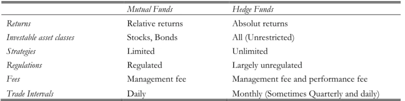
The differences between mutual funds and hedge funds have been described by Howells and Bain (2006). Hedge funds might for instance use leverage to increase their investment volumes above the initial amount invested by the funds investors. Moreover, the hedge fund fees are higher and have a different fee structure than the original mutual fund. For example, in the beginning, hedge funds could charge up to 2% of the managed capital in salary to the management and a bonus of around 20% of the net return per year. Today the salary fee is down to around 1% but the bonus system remains at the same level as before according to McRary (2002). The fee structure with the performance fee along with a gen-eral demand that managers should invest private money in the funds is a way to merge the investor and managers interest of not only high returns but also to reduce the risk taken by the management. Another difference is the low level of regulation, which enables hedge funds to increase their leverage even more by trading derivatives, other differences between hedge funds and mutual funds can be seen in Table 1.

Table 1 – Differences between mutual funds and hedge funds.

Mutual Funds Hedge Funds

Returns Relative returns Absolut returns

Investable asset classes Stocks, Bonds All (Unrestricted)

Strategies Limited Unlimited

Regulations Regulated Largely unregulated

Fees Management fee Management fee and performance fee

Trade Intervals Daily Monthly (Sometimes Quarterly and daily)

Investors usually refer to hedge funds as a single asset class but hedge funds are in reality very different depending on their investment strategies. Even though hedge fund managers classify their funds depending on the strategy, a fund could still use more than one strategy for their portfolio. Since this paper will examine the L/S equity hedge funds we will only present this strategy in detail. Figure 1 shows different hedge fund strategies proposed by Lhabitant (2004).

Figure 1 – Hedge fund strategies

Kat and Lu (2002) describe the Equity L/S funds as funds that take advantage of both the long and the short positions within the equity market and that it differentiates itself from the equity market neutral funds by taking on market risk, which means that the market risk is not always equal to zero. Fung and Hsieh (2004) have also found that the Equity hedge funds have exposure to the broad equity markets and especially to small cap stocks, mainly because it is easier for hedge fund managers to go long in small cap stocks and short in large cap stocks due to the problem of trade liquidity in small cap stocks.

The Swedish hedge fund market has been subject to decrease in the level of total managed value over the last two years, see Graph 1. This might be due to the reason that some Swe-dish hedge funds has been forced to close due to the instability within the financial markets in the years 2010 and 2011. For example, Brummer & Partners Sweden’s largest hedge

Hedge Fund Investment

Strategies

Tactical trading Equity long/short Event driven Relative value

arbitrage Others

* Global Macro

* Managed Futures * Global * Regional * Sectorial * Emerging * Distressed sec. * Risk arbitrage * Event driven * Convertible arb. * Fixed income arb. * Equity market neutral

* Multi strategy * Fund of Funds

fund provider had to close down two of their funds in 2011 due to low returns and man-agement problems.

Graph 1 – Managed Value

2.2

Standard & Poor Europe 350 index

Indexing as an investment form has become more popular over the last years in Sweden. An investor can today take advantage of the diversification that an index possesses by in-vesting in either contracts for differences (CFD’s) or index funds. The index fund is a sim-ple way for the investor to take advantage of the diversification that an index provides without the problems and transaction costs that arises if the investor should try to replicate the index by buying the securities within the index separately.

We will use the Standard & Poor Europe 350 (S&P Eur 350) to compare the different hedge funds towards since the main markets for the five funds used in this paper are the European and the Nordic stock markets in general (See Table 7, Appendix 2).

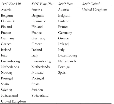
The S&P Eur 350 is an equity index consisting of 17 of the major markets within Europe. To determine the index constituents the index uses the biggest and most liquid stocks of the 10 sectors presented by the Global Industry Classification Standard. The 17 markets and the 10 sectors are presented in Table 8 and 9 in Appendix 2.

2.3

Value-at-Risk

In modern portfolio theory, investors will try to maximize their expected return over a giv-en risk level which is measured by the variance (Markowitz, 1952). But as the time has elapsed the need for risk management has increased and according to Ruppert (2004), J.P. Morgan introduced RiskMetrics to calculate the largest estimated loss that could occur over the next 24 hours. This risk measure came to be known as Value-at-Risk when it was made public in 1994(J.P Morgan, 1996).

The major breakthrough for VaR during the last decade has been due to the models ability to measure all types of risk in all types of financial securities even complicated portfolios

like hedge funds. The VaR is composed of two parameters the confidence level (1-α) and the holding period (T). VaR is then defined over these two parameters as the maximum loss over the given holding period at a certain confidence level.

2.3.1 Historical and Filtered Historical Simulation of Value-at-Risk

The historical simulation of Value-at-Risk, first introduced by Boudukh et al. (1998) and Barone-Adesi et al. (1998, 1999), is a risk simulation created from a historical sample of re-turns. Barone-Adesi et al. (1999) perform a back test analysis on the filtered historical simu-lation (FHS) where they tested 100,000 daily portfolios held by financial institutions and found that FHS is a validated model for risk measurement. FHS is an extension of the his-torical simulation (HS), except from only using the returns as the hishis-torical simulation the filtered historical simulation applies a statistical bootstrap to create a random draw from the empirical return.

But what are the main advantages with HS? The main advantage is that we do not have to make any assumptions about the return distribution or serial independence i.e. other VaR models such as the parametric linear model assumes that the returns are independent and identically distributed (iid). This is a huge simplification since most returns, especially hedge fund returns, exhibits excess kurtosis and negative skewness. Another advantage of the HS is that since we do not assume that the returns are iid it allows us to model volatility clus-tering, which is not possible in the linear parametric model. The relaxation of these as-sumptions about the parametric distribution allows us to model complicated risk behaviors direct from a historical sample and still include the dynamics of risk in a natural way. A substantial limitation of the HS is that if we apply a long time period of returns, it will cover many different market scenarios, which will bias our estimates and not reflect the current market conditions. The Monte Carlo Simulation (MCS) of VaR on the other hand uses historical returns but it does not assume that the return that led to our current VaR model is the one that will appear during our risk horizon. Instead it lets us generate thou-sands of simulated returns that could appear over our holding period. The FHS uses a mix of the HS and the MCS and lets us model volatility clustering and non-normal distributions over an historical sample.

3

Method

This section will describe the different statistical models and their respective formulas that we use. It will also give a more complete picture of the historical Value-at-Risk and the Expected tail loss measurements which are used to test our hypothesis.

3.1

ARMA

We will use an ARMA (p,q) process to model the serial dependence (Füss et al., 2006) in our mean equation (eq. 11). The ARMA (p,q) process consists of two parts, an regressive and a Moving average part (Lütkepohl and Krätzig, 2004). Where the Auto-regressive part, AR(p), is of the p:th order.

∑

Where c represents our constant, is our parameter up till order p and is the error term, which is considered to be white noise.

The Moving Average, MA (q), is the second part of the ARMA (p,q) process where q has the same interpretation as p i.e. q is the order of Moving Average parts. Where the order represents number of lagged terms in our AR (p) and MA (q) models. The MA (q) model is represented by the following formula:

∑

Where represents our expectations of is our parameter up till order p. is the error term (white noise) for l number of periods back and is white noise.

The ARMA (p,q) model is then represented by a formula consisting of equation 1 and 2:

∑ ∑

The number of p and q orders respectively is then chosen by minimizing the Akaike and Schwarz information criteria’s. We will put a restriction on the number of orders for p and q in our ARMA (p,q) model where we will allow for a maximum of three lags. This is due to the reasons presented by Ruppert (2004) who questions the use of lags to far way since there is no economic theory explaining why returns should be affected by a return to far back. In our case three periods back since we question that monthly data would have serial dependence for longer than three periods back.

3.2

GARCH models

Alexander (2008) argues that the best way to obtain the needed volatility estimates for the filtered historical VaR calculation is to use an asymmetric GARCH-model. When selecting a proper GARCH model for our time series of returns we have to choose a model that fits our data frequency and also our both asset types, funds and indices. Since our data contains equities, Alexander (2008) suggests an asymmetric GARCH-model since the relationship between the volatility of returns and the actual return is assumed according to Engle and Ng (1993) to have a negative relationship. This will cause large increases in equities market volatility to cause also large decreases in the equity return, which is also valid the other way around. This is because of the leverage effect that arises when the value of equity falls (the price of an asset goes down) causing the debt-equity ratio to rise because of debt-financings long adjustment time.

The definition of the conditional mean and the conditional variance in a time series of re-turns is equal to the mean and the variance of a random variable given the information of another random variable:

[ | ] [ | ]

Where is the conditional mean of our returns labeled at time t. is the conditional variance and is known information about another random variable at t-1. This gives that our time series of returns denoted will be generated by:

√ Where is price innovations (residuals) at time t.

We expect that the mean and the variance of our price innovations will be equal to 0 and 1 respectively, given the information about another random variable at t-1.

[ | ] and:

[ | ] The symmetric normal GARCH (p,q) model is built on two equations, the conditional

mean equation and the conditional variance equation. It also assumes that the time series of returns is a composition of the conditional mean and the price innovations at time t.

We will follow Engle (1982) assuming that the conditional distribution of the error term is normally distributed with a mean equal to zero.

|

Füss et al. (2006) propose that the mean equation for the GARCH (p,q) model should be modeled by an ARMA- process to account for serial dependence in the returns for hedge funds, which is caused by infrequent trading (monthly trading). They further propose the following ARMA process for the time series of hedge fund returns:

∑ ∑

The conditional variance in the GARCH (p,q) model is according to Bollerslev (1986) a function of the past conditional variance and the squared past price innovations at time t-1. This gives us the formula for the conditional variance:

Where is equal to the GARCH error term and measures the conditional volatility’s sensi-tivity to market shocks. The parameter is the GARCH lag parameter, which measures the persistence in the conditional volatility without respect to market shocks. A rule of thumb is that when is above 0.9 it will take long time for the volatility to return to its mean. The constant parameter divided by (1- - ) measures the long-term volatility within the mar-ket.

We have to put restrictions on the parameters in the above equation to make sure that neg-ative variances are excluded. The restrictions are as follows:

And according to Bollerslev (1986) the following condition has to be met in order to en-sure stationarity:

The asymmetric EGARCH model introduced by Nelson (1991) differentiates itself from the symmetric GARCH model by formulating the conditional variance in logarithms.

(|

|

)

Since the EGARCH is a log transformation, all the previous restrictions which are imposed on the symmetric GARCH model becomes irrelevant. Although positive values for is necessary to model the volatility clustering and in order to interpret the leverage effect, symbolized by , the parameter needs to have a negative sign and be significant.

3.3

Filtered Historical Simulation

The main reason to use a Filtered Historical Simulation (FHS) instead of the more simple Historical simulation is because the FHS allows us to create risk measures that are valid and consistent with the current market risk. But the FHS volatility adjustment also makes our sample of data more close to being iid, which means that our VaR estimates becomes less sensitive to the relatively small sample size that we use in this paper.

The FHS also allows us to generate extreme events, which not might be present in our his-torical data, this property will not create leptokurtic tails for the return distribution. This al-so allows FHS to use a shorter historical data series than the more simple HS method, which was proven by Barone-Adesi et al. (1999).

We start our FHS by finding the GARCH annual volatility on the 29th of February 2012 by taking the square root of the variance at this point in time. This will give us the monthly volatility on the last day of our sample when the VaR is estimated.

The next step in our FHS is to find the monthly log return on our last observation, 29th of February 2012, which is our starting value. The simulated daily log returns over the risk horizon is then equal to our estimated standard deviation multiplied by an independent random variable from our standardized empirical returns obtained by a statistical bootstrap. By repeating this for 96 simulations it will create a simulated return distribution where the FHS VaR is obtained by taking the -quantile of this distribution.

3.4

Expected Tail Loss

We use expected tail loss as a complement to the FHS VaR since the VaR measure does not tell us anything about the loss that can occur if the VaR is exceeded. The ETL or Con-ditional Value-at-Risk (CVaR) as it is called provides us with this information. Another good thing with the ETL is that it adds the sub additive condition, which the FHS VaR is argued to lack (Szegö, 2004).

| Where:

Expected Tail Loss

The h-day return on the portfolio The 100α h-day VaR in percentage form

4

Data

This chapter will provide a description of the data used to find the assets respective Value-at-Risk and Ex-pected Tail Loss estimates.

4.1

Description of data

This study uses a data set with historical monthly returns from five different Swedish hedge funds and Standard & Poors index Europe 350. I have chosen the five largest Swedish Eq-uity L/S hedge funds with respect to the managed value of the funds. The output from the ranking of hedge fund sizes is then filtered to find the funds with historical returns that reach over more than eight years.

4.2

Sample size and sources

The sample size of our data is limited due to the limited amount of Swedish hedge funds with available historical returns of more than eight years. We will use the monthly after-fee returns between March 2004 until February 2012, which will give us 96 monthly observa-tions/fund. The choice of time period is made with respect to the Historical Simulation of VaR, because we want to capture as many infrequent events and market conditions as pos-sible to base our VaR estimation and ETL on. The time period captures both the bull mar-kets before the financial crises of 2007 and the bear marmar-kets that followed.

The data for the hedge funds are collected from the chosen hedge funds monthly reports and their respective NAV-values. The data of monthly returns for the S&P Europe 350 in-dex was obtained through contact with S&P.

5

Empirics

This section aims to use the theories and models described in section 2 and 3 on our time series of returns in order to test the hypothesis stated in section 1.3. The section is divided into six parts, which are presented in a chronological order.

5.1

Hedge fund selection

The hedge fund selection was conducted through collection of the hedge funds managed value and then sorted after size as can be seen in Appendix 1. In order to ensure as large sample size as possible the restriction of historical returns of no less than eight consecutive years where imposed. This restriction excluded one fund, Archipel, from the selection. The funds in this paper all has a managed fund value of over 1.5 billion SEK and are registered in Sweden.

5.2

Descriptive statistics

The type of data used in this paper is a time series of monthly logarithm returns between March 2004 and February 2012 this time span gives us 96 observations per fund/index. Table 2 is an overview and summation of the assets returns and their respective characteris-tics.

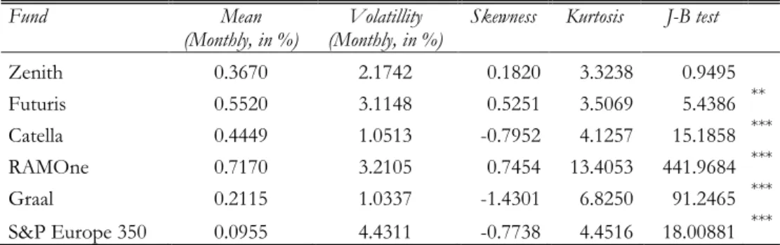
Table 2: Descriptive statistics

Fund Mean

(Monthly, in %) (Monthly, in %) Volatillity Skewness Kurtosis J-B test

Zenith 0.3670 2.1742 0.1820 3.3238 0.9495 Futuris 0.5520 3.1148 0.5251 3.5069 5.4386 ** Catella 0.4449 1.0513 -0.7952 4.1257 15.1858 *** RAMOne 0.7170 3.2105 0.7454 13.4053 441.9684 *** Graal 0.2115 1.0337 -1.4301 6.8250 91.2465 *** S&P Europe 350 0.0955 4.4311 -0.7738 4.4516 18.00881 ***

Notes: Figures are based on monthly returns between March 2004 and February 2012 (96 observations). ***, ** and * represents the significance levels for the J-B test(rejection of a normal distribution for the re-turns)at the 99, 95, 90% confidence level.

Since we use monthly data and also presents the forthcoming FHS VaR as the maximum expected loss over the next month the mean return and the volatility is presented as monthly values in percentage terms. We can see that all hedge funds has considerably high-er monthly returns than the index whhigh-ere the hedge funds range is between 0.21-0.71% re-turn on average while the S&P Europe 350 has a monthly average rere-turn of 0.09%.

The hedge funds volatility is lower than the index and the difference between the hedge fund with the highest volatility and the index is almost one percent per month. This is an indication that the hedge funds have a lower downside-risk than the index. But the volatili-ty is not a defendable method to use as a risk measurement if the returns do not exhibits a normal distribution.

All assets exhibit positive excess kurtosis, which indicates that the returns are not normally distributed although Zenit and Futuris hold low values of excess kurtosis. This finding is in line with the findings of Kat and Lu (2002) who find that the individual hedge fund return exhibits excess kurtosis. This is also confirmed by the Jarque-Bera test for normality and its respective significance level, which makes it possible to reject the null hypothesis of nor-mally distributed returns for all assets except Zenit and Futuris at the 95%confidence level. The non-normal distribution and the leptokurtic tails are confirming the existence of vola-tility clustering and ARCH effects within our sample.

5.3

ARMA modeling

As described in Equation (11) we use autocorrelation and an ARMA structure to model the mean equation due to the serial dependence caused by infrequent trading. We use a model selection process, which is based on the autocorrelation function (ACF) and the partial au-tocorrelation function (PACF) to find an optimal lag structure that captures the serial cor-relation within our time series.

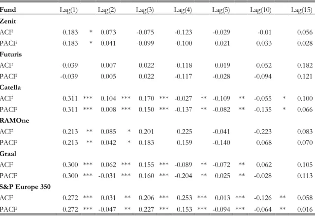
Table 3: Autocorrelation

Fund Lag(1) Lag(2) Lag(3) Lag(4) Lag(5) Lag(10) Lag(15) Zenit ACF 0.183 * 0.073 -0.075 -0.123 -0.029 -0.01 0.056 PACF 0.183 * 0.041 -0.099 -0.100 0.021 0.033 0.028 Futuris ACF -0.039 0.007 0.022 -0.118 -0.019 -0.052 0.182 PACF -0.039 0.005 0.022 -0.117 -0.028 -0.094 0.121 Catella ACF 0.311 *** 0.104 *** 0.170 *** -0.027 ** -0.109 ** -0.055 * 0.100 PACF 0.311 *** 0.008 *** 0.150 *** -0.137 ** -0.082 ** -0.135 * 0.066 RAMOne ACF 0.213 ** 0.085 * 0.201 0.225 -0.041 -0.223 0.083 PACF 0.213 ** 0.042 * 0.183 0.159 -0.140 0.068 0.070 Graal ACF 0.300 *** 0.062 *** 0.155 *** -0.089 ** -0.072 ** 0.062 0.105 PACF 0.300 *** -0.031 *** 0.160 *** -0.204 ** 0.025 ** -0.028 0.113 S&P Europe 350 ACF 0.272 *** 0.031 ** 0.206 *** 0.253 *** 0.013 *** -0.126 ** 0.058 PACF 0.272 *** -0.047 ** 0.227 *** 0.153 *** -0.094 *** -0.064 ** 0.016 Notes: Figures are based on monthly returns between March 2004 and February 2012 (96 observations). ***, ** and * represents the significance levels for the ACF and PACF at the 99, 95, 90% confidence level. Table 3 presents the different assets autocorrelation coefficients and their respective signif-icance levels. The negative values for ACF and PACF means that the volatility of the un-smoothed sample would decrease over time. We can also see that most assets exhibits high autocorrelation coefficients and they are significant above Lag (5). Catella, Graal and S&P Eur 350 indicates autocorrelation up to Lag (5), RAMOne up to Lag (2) and Zenit up to

Lag (1). This indicates that there is autocorrelation present between the returns up to 5 riods back for Catella, Graal and S&P Eur 350, two periods back for RamOne and one pe-riod for Zenit. This is in line with the findings of Brook and Kat (2002) who find that there is significant degree of autocorrelation present in hedge fund returns. The lag structure of the funds indicates that the best ARMA structure for Catella, Graal and S&P Eur 350 might be between ARMA (1,1) and ARMA (5,5), RamOne between ARMA (1,1) and ARMA (2,2) and Zenit should be modeled with an ARMA (1,1) structure. Futuris doesn’t exhibit any autocorrelation and is therefore modeled with a constant for the mean equa-tion. The lack of autocorrelation for Futuris is not a problem since we still have Leptokur-tic tails, which allows the usage of GARCH/EGARCH models.

5.4

GARCH estimations

GARCH/EGARCH estimations are built on a mean equation and a variance equation, see Equation (4) and (5), where we obtain the mean equation through an ARMA process (eq. 11). The selection of an ARMA (p,q) model and its respective number of autoregressive (p) and moving average(q) parts are chosen by estimating GARCH parameters with different ARMA structures and thereafter choose the model which minimizes the Akaike and Schwarz information criteria’s (AIC,SIC) and maximizes the significance level.

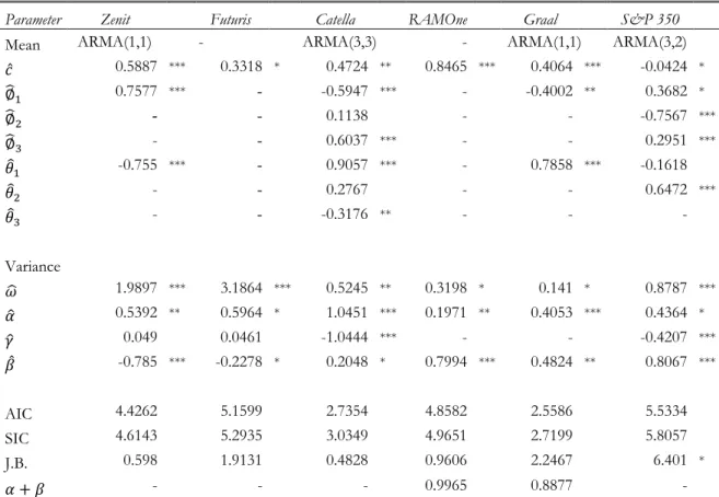
Table 4: GARCH parameters

Parameter Zenit Futuris Catella RAMOne Graal S&P 350

Mean ARMA(1,1) - ARMA(3,3) - ARMA(1,1) ARMA(3,2)

̂ 0.5887 *** 0.3318 * 0.4724 ** 0.8465 *** 0.4064 *** -0.0424 * ̂ 0.7577 *** - -0.5947 *** - -0.4002 ** 0.3682 * ̂ - - 0.1138 - - -0.7567 *** ̂ - - 0.6037 *** - - 0.2951 *** ̂ -0.755 *** - 0.9057 *** - 0.7858 *** -0.1618 ̂ - - 0.2767 - - 0.6472 *** ̂ - - -0.3176 ** - - - Variance ̂ 1.9897 *** 3.1864 *** 0.5245 ** 0.3198 * 0.141 * 0.8787 *** ̂ 0.5392 ** 0.5964 * 1.0451 *** 0.1971 ** 0.4053 *** 0.4364 * ̂ 0.049 0.0461 -1.0444 *** - - -0.4207 *** ̂ -0.785 *** -0.2278 * 0.2048 * 0.7994 *** 0.4824 ** 0.8067 *** AIC 4.4262 5.1599 2.7354 4.8582 2.5586 5.5334 SIC 4.6143 5.2935 3.0349 4.9651 2.7199 5.8057 J.B. 0.598 1.9131 0.4828 0.9606 2.2467 6.401 * - - - 0.9965 0.8877 -

Notes: Figures are based on monthly returns between March 2004 and February 2012 (96 observations). ***, ** and * represents the significance levels for the estimated parameters at the 99, 95, 90% confidence level. Significance levels for J.B.-test are for rejection of a normal distribution.

We could see from Table 3 that Futuris does not have any autocorrelation between the re-turns and this is also confirmed by the output from the different ARMA/GARCH/EGARCH models, which minimizes the Akaike and Schwarz selection criteria’s when the mean equation consists of a single constant. The output from Table 3 is also consistent with the findings in Table 4 for Zenit, Catella, Graal and S&P Eur 350, which are modeled with an ARMA (1,1), ARMA (3,3), ARMA (1,1) and ARMA (3,2) re-spectively. The only fund, which is not consistent with the findings in Table 3, is RAMOne that shows signs of significant autocorrelation in Lag (1) but minimizes the AIC and SIC with one constant in the mean equation. The restriction of number of lagged terms in the mean equation is also fulfilled, since no asset has above three lags.

The choice between GARCH/EGARCH is made by minimizing the AIC, SIC and con-firming the signs of the restricted parameters. All the assets alphas are positive which is a result of our modeling of volatility clustering i.e. ARCH effects is present in our time series of returns. Zenit, Futuris, Catella and S&P Eur 350 are modeled with an asymmetric EGARCH model, which captures the leverage effect previously described, but only Catella and S&P Eur 350 shows significant signs of a leverage effect and the ̂ are negative which is a criterion for taking the estimated parameter into account. Zenit and Futuris show tive values for ̂ and they are not significant. This is also confirmed by looking at the posi-tive skewness values in Table 2 for Zenit and Futuris, Catella and S&P Eur 350 has a nega-tive skewness which confirms that there might be a leverage effect present within the time series (Füss et al. 2006).

For the assets where a symmetric GARCH model provides the best fit to the time series, the restriction that both ̂ and ̂ should be positive is fulfilled. The restriction to provide stationarity is also fulfilled since ̂+ ̂< 1. Although the sum is close to one for all the as-sets which uses symmetric GARCH modeling, which means that the volatility has a long memory, it will still be mean reverting but the process will take some time.

The Jarque-Bera test performed on the residuals shows that we cannot reject the null hy-pothesis that the residuals are normally distributed at the 95% confidence level. This indi-cates that the residuals are white noise containing no information about our process and our models provide god estimates of the parameters.

5.5

Filtered Historical Simulation of Value at Risk

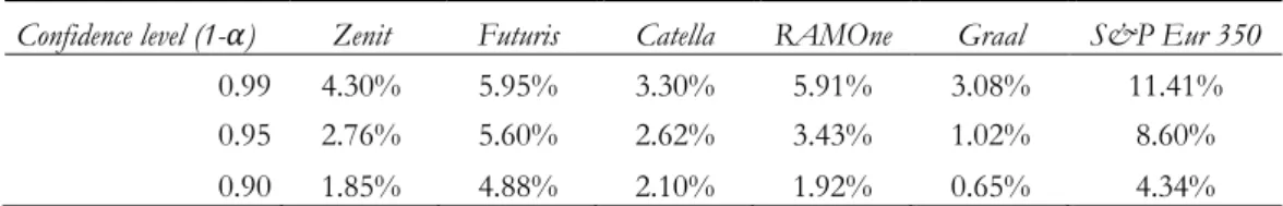
The results of the FHS VaR shows that all the funds have lower VaR than the index. The funds also seems to outperform the index with considerably lower downside-risk during the next period at all confidence levels except for the 0.90 level where the index shows a lower VaR than Futuris. The asset with the lowest VaR is Graal with a VaR of 3.08% at the 99% confidence level and the asset with the highest VaR is the index S&P Eur 350 with a VaR of 11.41% for the next period.

Table 5: FHS VaR

Confidence level (1- ) Zenit Futuris Catella RAMOne Graal S&P Eur 350 0.99 4.30% 5.95% 3.30% 5.91% 3.08% 11.41% 0.95 2.76% 5.60% 2.62% 3.43% 1.02% 8.60% 0.90 1.85% 4.88% 2.10% 1.92% 0.65% 4.34% Notes: Figures are based on monthly returns between March 2004 and February 2012 (96 observations).

5.6

Expected Tail Loss

To estimate the loss that can occur if the FHS VaR is exceeded we calculate the average of the percentiles below our VaR confidence level of our empirical return distribution.

Table 6: ETL

Confidence level (1- ) Zenit Futuris Catella RAMOne Graal S&P Eur 350 0.99 5.77% 7.01% 3.80% 10.95% 3.90% 13.03% 0.95 4.57% 6.05% 2.71% 7.17% 2.92% 11.76% 0.90 3.69% 4.93% 2.28% 5.01% 2.14% 9.20% Notes: Figures are based on monthly returns between March 2004 and February 2012 (96 observations). The result of the ETL is shown in Table 6 where we can confirm that if the VaR is exceed-ed it will result in a bigger loss. RAMOne has the biggest differences between the ETL and the VaR with almost 5 % at the 99% confidence level. But S&P Eur 350 still holds the largest number with an expected loss of -13.03% if the VaR is exceeded.

5.7

Analysis

The goal for ‘Equity L/S’ Hedge funds is to deliver absolute returns by taking advantage of both bear and bull markets through both long and short positions in equity. This also means that they should be able to minimize the market risk and not be dependent on bull markets to generate returns by using their specific strategy and thereby shift the efficient frontier to NW resulting in higher returns at lower risks. It is also the aim of the active management in hedge funds to generate not only absolute returns but also returns that is superior to the more passive form of investing, indexing. By analyzing our empirical results it is clear that the hedge funds confirms at least one part of our assumptions that the man-agers are able to reduce the market risk for the next holding period (month). As previously stated in section 5.5 the hedge funds are able to reduce the risk more than the index at all confidence levels except for Futuris at the 90% confidence level. This indicates that the correlation of hedge fund returns towards bonds and equity is not significant as Brooks and Kat (2002) stated. Instead it follows the results of Edwards (1999) and L’habitant (2004) which say that the hedge fund returns has low correlation to bonds and equity, since we came to the conclusion that Swedish Equity L/S hedge funds holds a lower market risk than our equity index in Table 5. Also the estimation of the loss that could occur if VaR was violated shows lower values for the market risk than the index.

ducing properties. The risk reducing properties and the low correlation to bonds and equity would make hedge funds an attractive vehicle for diversified portfolios.

There is still a risk of survivorship bias in our results since we only look at 5 out of 23 funds that have survived. The fact that an unknown amount of hedge funds has been shut down since their introduction is not taken into consideration. If these funds would have been among the five largest funds their current market risk might have changed our esti-mates. But on the other hand it is unlikely that one of the five largest equity funds has been shut down due to the findings of Gregoriou (2002) who points out the specifics of surviv-ing hedge funds where size of the fund is a main characteristic for survivorship.

Since the important parameters for both the GARCH and the EGARCH models all have significant values at 90% confidence level, we assume that our estimats of VaR and ETL are correct. And the J-B test for normality cannot reject the null hypothesis that our residu-als are normally distributed at the 95% confidence level, which confirms that our model captures all relevant information. The limitations of our test is that the estimates may be bi-ased due to the relatively small sample size, even though it is large enough to assume that the central limit theorem holds. Alexander (2008) also confirms that a smaller sample size can be used when it is the case of locked in funds, which it is in our case. It is also evident that the leverage effect modeled by the asymmetric EGARCH model was not present in all funds, which might be due to the funds abilities of short selling.

The high values of the VaR measure is due to the relatively long holding period (1 month), VaR is in the normal case calculated as the loss that could occur over the next day or week and rarely over the next month. Since the volatility over a month is larger than it is for a day or a week it comes natural that the VaR threshold would be higher in our case. It should be considered that VaR is a worst-case scenario and not an approximation of the holding periods actual losses. One could also believe that since we use historical data from a long time period an event that has occurred during the worst bear markets of 2009 could affect our estimation? The answer is yes it would if we had used the parametric estimation of VaR. This is a reason to use the FHS where we capture the volatility with a statistical bootstrap and creates a new return distribution from where the volatility is estimated. To summarize our findings of Swedish Equity L/S hedge funds ability to reduce the mar-ket risk by applying the strategy of both long and short positions. We can see that the hedge funds used in this paper actually has a lower market risk exposure than the index. The funds also have a smaller ETL, which indicates that the funds volatility is lower than the index. This implies that the fund managers are able to reduce risk with their strategies of short and long positions.

6

Conclusion

The purpose of this thesis was to see if Swedish equity L/S hedge funds presents a lower market risk than the index Standard & Poor Europe 350 by using strategies such as long and short positions in equity. The need for risk reducing assets has become more evident in the last few years of financial disturbances and even though the Swedish market has seen a decline in the amount managed by hedge funds, investors need assets that can reduce mar-ket risk.

The results show that all of the examined hedge funds have lower market risk than the in-dex except for one fund at the 90 % confidence level for the 1-month holding period. We further estimated the maximum loss that could occur if the VaR is exceeded. The conclu-sion made from the estimation of ETL was that we could see if the VaR is exceeded, all hedge funds would have presented a lower market risk than the index. These findings make the examined Equity L/S hedge funds a suitable choice for risk-averse investors in highly volatile markets due to the funds risk reducing properties.

A suggestion for future research could be to examine a larger proportion of the hedge fund market and also include other strategies to see whether this is a specific characteristic for Equity L/S hedge funds or if it is applicable to all investments styles. And if possible a study with daily data which would increase the accuracy of the test.

References

Ackerman C, McNally R, Ravenscraft D, 1999, The performance of Hedge Funds: Risk, Return and Incentive, Journal of Finance, vol. 54, pp. 833-874

Alexander C, 2008, Market Risk Analysis II – Practical Financial Econometrics, John Wiley & Sons Ltd, Chichester

Alexander C, 2008, Market Risk Analysis IV – Value-at-Risk Models, John Wiley & Sons Ltd, Chichester

Anderlind P, Dotevall B, Eidolf, Holm M, Sommerlau P, 2003. Hedge fonder. Lund: Academia Adacta AB

Artzner P, Delbaen F, Eber J.M, Heath D, 1997, Thinking Coherently, Risk, vol. 10(11), pp. 68-71.

Artzner P, Delbaen F, Eber J.M, Heath D, 1999, Coherent Measures of Risk, Mathematical Fi-nance, vol. 3(9), pp. 203-228.

Barone-Adesi G, Bourgoin F, Giannopoulos K, 1998, Don’t Look Back, Journal of Risk, vol. 11, pp. 100-103

Barone-Adesi G, Giannopoulos K, Vosper L, 1999, VaR Without Correlations for Non-Linear Portfolios, Journal of Futures Markets, vol. 19, pp. 583-602.

Basel Committee on Banking Supervision, 2005, Amendment to the capital accord to incorporate market risks, http://www.bis.org/publ/bcbs119.htm, viewed February 2012

Bollerslev T, 1986, Generalized autoregressive conditional heteroskedasticity. Journal of Economet-rics, vol. 31, pp.307-327

Boudoukh J, Richardson M, Whitelaw R, 1998, The best of both worlds- A hybrid approach to cal-culating Value at Risk, Risk, vol. 11(5), pp. 64-67

Brooks C, Kat H, 2001, The statistical properties of Hedge Fund Index Returns and their implications for investors, Alternative Investment Research Center, Working Paper number:0004 Brown S, Goetzmann W.N, 1995, Performance Persistence, Journal of Finance, vol. 50, pp.

679-698

Brown S, Goetzmann W.N, Park J, 2001, Careers and Survival: Competition and Risk in Hedge Fund and CTA Industry, Journal of Finance, vol. 53(5), pp. 1869-1886

Daníelsson J, Jorgensen B, 2005, Subaddativity Re-Examined: The Case for Value-at-Risk; FMG Discussion Paper, London School of Economics

Duffie D, Pan J, 1997, An overview of value at risk, Journal of derivatives, vol 4, pp. 7-49 Edwards F, 1999, Hedge Funds and the Collapse of Long-Term Capital Management, Journal of

Edwards F, Liew J, 1999, Hedge Funds and Managed Futures As Asset Classes, The Journal of Derivatives, Summer (1999), pp. 45-64

Engel R.F, 1982, Autoregressive conditional heteroscedasticity with estimates of the variance of UK infla-tion, Econometrica, vol. 50, pp. 987-1007

Engel R.F, 1990, Stock volatility and the crash of ’87:Discussion, The review of Financial Studies 1990, vol. 3(1), pp. 103-106

Engel R.F, Ng V.K, 1993, Measuring and testing the Impact of News on Volatility, Journal of Fi-nance, vol. 48, no 5, pp. 1749-1778

Fung W, Hsieh D.A, 2000b, Performance Characteristics of Hedge Funds and CTA Funds: Natural Versus Spurious Biases, Journal of Financial and Quantitative Analysis, vol. 35(3), pp. 291-307

Fung W, Hsieh D.A, 2004, Extracting Portable Alphas from Long/Short Hedge Funds, Journal of Investment Management, vol. 2(4), pp.1-19

Füss R, Kaiser D.G, Adams Z, 2006, Value at risk, GARCH modelling and the forecasting of hedge fund return volatility, Journal of derivatives & Hedge Funds, vol. 13(1), pp. 2-25 Gregoriou G, 2002, Hedge Fund Survival Lifetimes, Journal of Asset Management, vol. 3(3),

pp. 237-252

Howells P, Bain K. 2005, The Economics of Money, Banking and Finance: A European Text, Pear-son Education, Essex

Jaeger L, Wagner C, 2005, Factor Modeling and Benchmarking of Hedge Funds: Can passive Invest-ments in Hedge Fund Strategies Deliver?, Journal of Alternative Investment, vol. 8, pp. 9-36

J.P Morgan. 1996, RiskMetrics – Technical Document Fourth edition, New York,

http://pascal.iseg.utl.pt/~aafonso/eif/rm/TD4ePt_2.pdf, Viewed February 2012 Kat H.M, Lu S, 2002, An Excursion Into the Statistical Properties of Hedge Fund Returns, Working

Paper, ISMA Center, University of Reading

Lhabitant F-S, 2001, Assessing Market Risk for Hedge Funds and Hedge Funds Portfolios, FAME, Working paper no. 24

Lhabitant F-S, 2004, Hedge Funds – Quantitative Insights, John Wiley & Sons Ltd, Chichester Liang B, 2000, Hedge Funds: The Living and the Dead, Journal of Financial and Quantitative

Analysis, vol 35(3), pp. 309-326

Lo A, 2001, Risk Management for Hedge Funds: Introduction and Overview, Financial Analysts Journal, vol. 57(6), pp. 16-33

Markowitz H.M, 1952, Portfolio Selection, Journal of Finance, vol. 7(1), pp.77-91

McNeil A.J, Frey R, Embrechts P, 2005, Quantative Risk Management: Concepts, Techniques and Tools, Princeton University Press, Princeton

McRary S, 2002, How to create & manage a hedge fund – A professional’s guide, John Wiley & Sons Ltd, Chichester

Nelson D.B, 1991, Conditional Heteroskedasticity in asset Returns: A New Approach, Econometri-ca, vol. 59(2), pp.347-370

Nordén P, 2008, A brighter future with lower transaction costs?, Journal of Futures Markets, vol. 29, pp. 775–796

Pérignon C & Smith D, 2006, The level and quality of Value-at-Risk disclosure by commercial banks, Journal of Banking & Finance, vol. 34, pp. 362-377

Pritsker M, 2001, The Hidden Dangers of Historical Simulation, Journal of Banking & Finance, vol 30, pp. 561-582

Ruppert D. 2004. Statistics and Finance. An Introduction. Springer-Verlag, New York

Strömqvist M, 2008, Hedge Funds and International Capital Flows, EFI - The Economic Research Institute at Stockholm School of Economics, No. 743

Strömqvist M, 2009, Hedgefonder och Finansiella Kriser, Penning och valuta politik:

Swedish National Bank, Vol. 1/2009

http://www.riksbank.se/Pagefolders/39893/2009_1_pv_sv.pdf Viewed May 2012 Szegö G, 2004, Risk measures for the 21st _{Century, John Wiley & Sons Ltd, Chichester}

Ziemba W.T. 2003. The Stochastic Programming Approach to Asset, Liability, and Wealth Manage-ment. The Research Foundation of The Association for Investment Management and Research, Charlottesville

Appendix 2

Table 7 – Equity markets

Fund Market Main Focus Zenit Europe Nordics Futuris Europe

Graal Europe United Kingdom Catella Nordics

RAMOne Nordics

Table 8 – Constituting Countries

S&P Eur 350 S&P Euro Plus S&P Euro S&P United Austria Austria Austria United Kingdom Belgium Belgium Belgium

Denmark Denmark Finland Finland Finland France

France France Germany

Germany Germany Greece

Greece Greece Ireland

Ireland Ireland Italy

Italy Italy Luxembourg

Luxembourg Luxembourg Netherlands Netherlands Netherlands Portugal

Norway Norway Spain

Portugal Portugal

Spain Spain

Sweden Sweden

Switzerland Switzerland

United Kingdom

Table 9 – Global Industry Classification Standard, Sectors

Sectors Energy Materials Industrials Consumer Discretionary Consumer Staples Health Care Financials Information Technology Telecommunication Services Utillities