ADVANCED PHENOLOGY OF HIGHER TROPHIC LEVELS SHIFTS APHID HOST PLANT PREFERENCES AND PERFORMANCE
by
MARIA L MULLINS
B.S. University of Montana, 2010
B.A. University of Montana, 2010
A thesis submitted to the Graduate Faculty of the
University of Colorado Colorado Springs
in partial fulfillment of the
requirements for the degree of
Master of Sciences
Department of Biology
© 2019 Maria L Mullins All Rights Reserved
ii
This thesis for the Master of Sciences degree by
Maria L Mullins
has been approved for the
Department of Biology
by
Emily Mooney, Chair
Shane Heschel
Cerian Gibbes
iii Mullins, Maria L (M.Sc., Biology)
Advanced phenology of higher trophic levels shifts aphid host plant preferences and performance Thesis directed by Assistant Professor Emily Mooney
ABSTRACT
The abundance of insect herbivores, such as aphids, is mediated by interactions with higher and lower trophic levels. Bottom-up processes can affect the phloem sap quality that aphids depend on for food, while natural enemies exert top-down control to directly and indirectly impact the success of aphids. This research asks (1) how phenological change across trophic levels affects host plant quality and selection for aphids, and (2) what mechanisms drive the ability of aphids to distinguish between potential hosts. We used a tri-trophic system to investigate these questions. Ligusticum porteri is a robust, perennial herb that hosts the sap-feeding aphid Aphis asclepiadis, and intraguild predators (Lygus spp.—lygus bugs) in a subalpine system near Gothic, Colorado. We used long term observational data to discover that species in this tri-trophic system respond
differently to phenological cues, and when phenology of Lygus hesperus is advanced on early snowmelt years, aphid colonies do not reach high densities. These unique
phenological responses to climatic cues can impact aphid abundance through changes to host plant quality and the host plant selection process. We used behavioral choice assays to assess how advanced L. hesperus phenology influences aphid host plant selection using plants experimentally colonized by L. hesperus compared to controls. More alate aphids chose to land and reproduce on lygus bug free control plants, indicating overall
iv
avoidance of plants with prior herbivory by L. hesperus. However, this preference did not correlate with aphid performance when we compared aphid relative growth rates between treatments. This suggests that advanced phenology of L. hesperus may impact aphid populations more through direct predation rather than reductions in host quality. These predation effects could be mediated if aphids can detect natural enemy presence during host selection. We measured plant cues involved in host selection and found differences in volatile composition from plants with prior L. besperus feeding compared to L.
hesperus free control plants. Such differential host selection could demonstrate that
aphids may be able to detect enemy free space using volatile cues. Our results indicate that higher trophic interactions both directly and indirectly influence aphid abundance. This work highlights the importance of including multi-trophic interactions in studies examining insect herbivore abundance.
v
ACKNOWLEDGEMENTS
This research was funded by the National Science Foundation with a grant awarded to Emily Mooney (NSF Award ID #: 1655914), and a National Science
Foundation grant that was awarded to the Rocky Mountain Biological Laboratory (DBI-1624073). Graduate student work was also partially funded by the Colorado Native Plant Society Marr Fund, the University of Colorado, Colorado Springs Graduate Research Stipend, and the Rocky Mountain Biological Laboratory Graduate Research Fellowship. The research was completed at the Rocky Mountain Biological Laboratory with help from the RMBL Research Committee and Jennie Reithel.
I would like to thank Dr. Emily Mooney for her valuable contributions to this project, as well as her support and guidance throughout the research process. Jim Den Uyl and the rest of the research team helped immensely in the field for which I am very grateful. Dr. Shane Heschel, Dr. Cerian Gibbes, and Dr. Diane Campbell provided valuable insight and feedback. I would also like to thank my partner Sam and my family and friends for their endless support and encouragement.
vi
TABLE OF CONTENTS
CHAPTER
I. INTRODUCTION…….………..……1
II. METHODS AND MATERIALS………...7
III. RESULTS………..19
IV. DISCUSSION………29
vii
LIST OF TABLES
TABLE
1. Results from the multiple analysis of variance performed to analyze composition of 6 sugars within collected aphid honeydew………...………….22
2. Results from spectral data analysis, aggregated by phenological stage of L.
porteri. Wavelength of peak indicates what region along the aphid visible
spectrum contained the highest reflectance peak. The reflection intensity
associated with that peak is also reported, as well as the total brightness which is the area under the curve for the largest peak between 500-600 nanometers…...23
3. Results table from volatile analysis. Verified compounds are identified by its Chemical Abstract Service (CAS) number, the biosynthetic class which is belongs to, and its relative abundance among both plant treatments………..25
4. Relative abundance of each chemical compound class for both plant treatments, grouping all verified compounds……….………..…………27
viii
LIST OF FIGURES FIGURE
1. Diagram showing experimental design of behavioral aphid choice
assays……….11 2. Differential insect response across trophic levels to snow melt date. Aphids
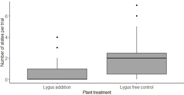
respond inversely to year-to-year variation in snowmelt, while lygus respond directly to this phenological cue (χ2 = 27.73, P< 0.001)…………..…………..…19 3. Boxplots showing the preference of A. asclepiadis alates to plants with L.
hesperus colonization and L. hesperus free control plants in 19 behavioral choice
assays. Permutation tests showed significance preference for plants without L.
hesperus (z = 2.26, P = 0.024). Bold lines show the median of each group, the
whiskers indicate maximum and minimum values, and circles show outliers...21 4. Curve of spectral data for each phenological stage of L. porteri. Solid red lines
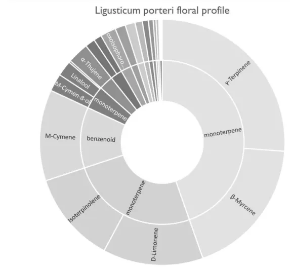
show the peak of max reflectance for each stage, which occurs at 559 nanometers. The scale of the y-axis shows reflection intensity across phenological stages..…23 5. Pie chart displaying the relative abundance of chemical compounds found in L.
porteri. The outer ring shows individual compounds, and the inner ring classifies
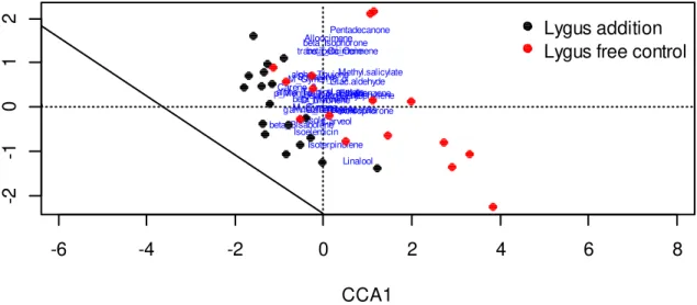
each compound according to its biosynthetic class.………..………26 6. Constrained correspondence analysis plot displaying the variation of chemical
compounds and how differences in relative abundance amongst treatments
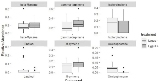
explains part of the overall variation in the emissions data…...….27 7. Boxplots displaying the 6 chemical compounds which had the highest differences
ix
significant (P-value > 0.05), but they did contribute the most to the variation between treatments……….………28
CHAPTER I
INTRODUCTION
Changes to insect herbivore populations can have rippling effects throughout their communities and consequently, ecologists are examining insect herbivore abundance in the context of global change. Insect herbivores provide important ecosystem services such as nutrient cycling, make up the base of most terrestrial food webs, and alter plant composition and abundance (Crawley, 1983; Belovsky & Slade, 2000). Many studies attempting to predict the future of herbivore abundance have focused on direct effects of rising temperatures on ectotherms based on latitude and their physiological thermal tolerances (Deutsch et al., 2008). Corresponding to observations from past warming events, models generally predict a rise in insect herbivory with continued warming (Blois, Zarnetske, Fitzpatrick, & Finnegan, 2013). However, abiotic variables alone are not enough to draw conclusions about effects of global warming on insect herbivores; biotic interactions among host plants and higher trophic levels need to be addressed on a system specific scale (Karban, Grof-Tisza, & Holyoak, 2017).
Two factors that interact with insect physiological responses to climate variables are (1) host plant quality (i.e. bottom-up control) and (2) top-down control from higher trophic levels. Host plant quality may be impacted by responses to drought and
temperature, which can cascade up to primary consumers such as aphids (De Sassi, Lewis, & Tylianakis, 2012). Alternatively, higher trophic levels can directly impact herbivore populations through predation, and indirectly impact herbivores through competitor-induced host plant defenses (Mooney, Pratt, & Singer, 2012). A recent meta-analysis found that sap-sucking herbivores are more constrained from top-down than
bottom-up forces, but historically their dependence on their host plant for nutrition has received the most attention (Vidal & Murphy, 2018). Likely both host plant quality and natural enemies interact to explain herbivore abundance and distribution patterns. Currently, including multi-trophic interactions in manipulative experiments is seen as necessary to achieve ecological validity, especially within the framework of continued global warming (Nakazawa & Doi, 2012).
Climate will directly impact each of these trophic levels, and thus, interactions between species is mediated by individual responses to phenological cues (Burkle,
Marlin, & Knight, 2013). Phenological mismatch between interacting species could result in a shorter period of overlap between antagonistic species, a longer period of overlap between mutualistic species, or vice versa (Both, Van Asch, Bijlsma, Van Den Burg, & Visser, 2009). Though less studied than plant-pollinator interactions, phenological mismatch can occur between host plants and their insect herbivores (Kharouba, Vellend, Sarfraz, & Myers, 2015). In some plants, foliar quality declines as the growing season progresses, resulting in a short window for larvae development to synchronize with bud break for feeding on optimal quality host plants (van Asch, van Tienderen, Holleman, & Visser, 2007). For example, (Jones & Despland, 2006) used egg hatch manipulations to reveal that the late hatching of caterpillars relative to aspen phenology leads to reduced insect growth. Other simulated warming experiments found greater relative phenological advances of host trees than that of caterpillar egg hatch, which resulted in increased phenological synchrony and a benefit to the caterpillar (Schwartzberg et al., 2014). The variation in these results indicate that the nature of phenological shifts differ among species and study systems; subject to both direct and indirect effects of climate change
(Rosenblatt & Schmitz, 2016). Again, most of these studies involve interactions between host plants and primary consumers, but consequences of phenological differences
between herbivores and their natural enemies are much less studied. These too have the potential to greatly impact herbivore populations both through changes in the timing of overlap with predators, or indirectly through plant defenses induced by competitors (Denno et al., 2000). For instance, advanced phenology of a predator relative to an insect herbivore could result in less temporal overlap, increasing herbivore populations via decreased predation (Donnelly, Caffarra, & O’Neill, 2011). However, if host plant phenology tracks with that of the predator, this could simultaneously result in decreased plant quality, and increased predation pressure once the herbivore emerges.
This study examines this dynamic between phenology-mediated changes in resource quality and predator pressure on aphids, a widespread sap-feeding insect
herbivore. Phenological changes across trophic levels may impact the response of aphids through the host plant selection process. Host-plant selection cues—such as plant
reflected light and volatile emissions—may be changing in direct or indirect response to year-to-year variation in the timing and duration of snow cover. In our study system, the date of snow melt is an important phenological cue for host plants (Iler et al., 2013), and years with later snow melt are correlated with lower aphid abundance (Robinson et al. 2017). Locating a suitable host plant is an important process in the life cycle of aphids because apterous progeny are constrained to the host plant they are produced on (Dixon, 1977). The importance of host plant selection and its effects on aphid colony growth has been a major topic in the study of plant-insect interactions because of its implications for aphid colony establishment and success (Powell, Tosh, & Hardie, 2014; Wilson &
Leather, 2012). How natural enemies play a role in this process is much less studied, but recent research indicates that finding enemy-free space to oviposit may be as important, if not more, than locating a nutritionally superior host (Wilson & Leather, 2012).
Aphids choose to alight on host plants based visual cues associated with plant-reflected light, and olfactory cues from plant volatile emissions (Döring, 2014). As alates migrate, visual cues help guide them to their selective hosts, and they are attracted to certain wavelengths and intensity of the reflections they detect (Döring & Chittka, 2007). Plant reflectance is related to the timing of snowmelt as it predicts phenological
progression of L. porteri, and the color of L. porteri inflorescences change throughout flower development. This study takes an “aphids eye view” of how aphids’ habitat could be changing in response to this key climate change signal in arctic, alpine, and subalpine systems. The second plant cue aphids use to locate a suitable host is through the detection of host plant volatile emissions. Aphids use these scent blends to first find their host plant among a sea of green, and then to perceive the quality of a host plant based on complex volatile bouquets (Bruce, Wadhams, & Woodcock, 2005). Past research has highlighted the multiple roles of semiochemicals in plant-insect communication, with much attention paid to herbivore-induced host plant volatiles and predator attraction (Takabayashi & Dicke, 1996). It is well known that predators use herbivore-induced volatile emissions to locate plants with their aphid prey, however the ability of aphids to detect natural enemy presence through chemical footprints, or by volatile emissions induced by other
competitors is less understood (Hatano, Kunert, Michaud, & Weisser, 2008; Dicke, 2000). Herbivore preference for uninfested plants over plants with prior herbivory varies among insect species, but there are more examples of attraction than avoidance, and
aphids host selection response to interspecific competition is unclear (Bernasconi, Turlings, Ambrosetti, Bassetti, & Dorn, 1998; Dicke & Loon, 2000). These host plant signals have largely been studied in the context of finding ways to interfere with aphid host plant selection, such as visually or chemically camouflaging a crop of interest so that aphids are unable to locate and colonize the host (Döring, 2014), but more research involving aphid host choice in natural systems is warranted.
In this study, we determined the patterns and mechanisms by which phenological differences alter the abundance of interacting insect species. Our first objective was to assess whether we see differential responses to phenological cues across trophic levels using an 8-year observational dataset. We evaluated the response of aphids and their intraguild predator (lygus bugs) to the phenological cue of snow melt date. Secondly, we assessed whether advanced phenology of higher trophic levels affects colony growth of our focal aphid species. Using observational data, we tested how advances in lygus phenology predict aphid colony growth later in the season. Past work in this system reveals the importance of predation in determining aphid colony abundance across sites (Mooney et al., 2016). Additionally, lygus bug alteration of host plant chemicals via herbivory may be one mechanism affecting aphid population numbers on a given year (Rodriguez-Saona, Crafts-Brandner, Williams, & Paré, 2002). These observational patterns provide the biological relevance for the experimental portion of this study and will reveal how phenology-induced responses of higher trophic levels can interact with host plant quality (bottom-up effects) to determine aphid abundance.
Our third objective was to experimentally test the effects of prior natural enemy presence on aphid host plant preference and performance. We assessed the ability of
winged female aphids to detect the presence of an intraguild predator on their shared host plant. Through behavioral assays we asked whether winged females, given a choice between one plant colonized by an intraguild predator and one plant free of any insects, would support the enemy-free space hypothesis by choosing to land and oviposit on the plant free of intraguild predators. We then measured experimental aphid colony growth rates and sampled aphid honeydew to understand how competitor-induced changes in plant quality affect aphid colony growth, and to test whether aphid preference and performance are linked. We sampled plant reflectance to understand how phenological differences between host plant and herbivore may influence aphid host plant selection based on the colors aphids perceive during migration. Lastly, we sampled plant volatile emissions between plants which experienced prior herbivory by lygus bugs and those that did not. Insects use volatile composition as an important host plant cue during host selection processes, and changes to plant volatiles via competitor herbivory may affect host selection decisions. Combined these plant signals may identify possible mechanisms behind aphid host plant choice in this system.
CHAPTER II
METHODS AND MATERIALS Ligusticum - Aphis - Lygus System
In our study system near Crested Butte, CO, the aphid Aphis asclepiadis colonizes the umbel inflorescences of Ligusticum porteri. This host plant is a large, perennial herb in the Apiaceae family which grows abundantly in open meadows and aspen stands in this subalpine system (Terrell & Fennell, 2008). A. asclepiadis, synonymous with Aphis
helianthi (Lagos-Kutz, Favret, Giordano, & Voegtlin, 2016) is a host-alternating aphid
species that overwinters on Cornus sericea and migrates to L. porteri for the growing season (Addicott, 1978). A. asclepiadis has a holocyclic life cycle. Females reproduce parthenogenetically during the summer months and in the fall, they sexually reproduce overwintering eggs which emerge the next spring as the first asexual generation (Powell & Hardie, 2001). The aphids are polymorphic and produce alate morphs which are responsible for migration and new colony establishment. Lygus hesperus (Hemiptera: Miridae) is a sap-sucking herbivore that also feeds on the stems and inflorescences of L.
porteri (Robinson, Inouye, Ogilvie, & Mooney, 2017), along with other lygus species in
the tribe Mirini. Additionally, they are polyphagous predators whose nymphs and adults also feed on the instars of A. asclepiadis (Agustí & Cohen, 2000). A. asclepiadis also interacts with mutualist ants, who offer protection services in exchange for honeydew consumption (Addicott, 1979). A. asclepiadis is preyed upon by numerous predators such as ladybeetles and syrphid fly larvae and parasitized by various species of unidentified wasps (Desneux et al., 2009; K. A. Mooney, 2011).
Observational study
Species abundance in response to snow melt date
To test for differential responses to phenological cues across trophic levels, we used plant and insect census data collected from 10 replicate sites surrounding the Rocky Mountain Biological Laboratory (RMBL) near Gothic, CO. Details of the census
collection methods are described in (Robinson et al., 2017) and in total they compose an 8 year dataset from study years 2011-2018. We used a linear regression to assess the response of A. asclepiadis and L. hesperus to snowmelt date, which drives phenological processes of plants and insects in this subalpine system (Boggs and Inouye 2012). Snow melt date is described as the date of first bare ground seen by Billy Barr at a weather station located at RMBL (http://www.gothicwx.org/long-term-snow.html). The response variables for each species are (Y1) the number of host plants (out of 100) colonized by A.
asclepiadis in our last June census and (Y2) the number of host plants (out of 100)
colonized by L. hesperus in our last June census. We used data from the late June census because it is an important phenology and abundance response in this system (Robinson et al., 2017). These response variables are count data and have Poisson distributed errors, therefore we used a generalized linear model with the ‘glm()’ function included in the native stats package in R, and the ‘Anova()’ function in the car package tested the heterogeneity of slopes using an ANOVA type II sum of squares (R Core Team, 2017). We used R version 3.4.3 for these tests and all further statistical analysis (John et al., 2018; R Core Team, 2017).
Effects of advanced predator phenology on host plant quality
To assess whether advanced phenology of higher trophic levels affects host plant quality for aphids, we examined our long-term observational data to see whether L.
hesperus abundance in June predicts aphid colony success and colony growth rates later
in the season. There is evidence suggesting that other sap feeding herbivores induce reductions in plant quality that may adversely impact the success of later-colonizing insect species, however most research on this subject has been with leaf chewing
herbivores (Denno et al., 2000). From prior experimentation in our system, we know that
L. hesperus feeding reduces both chlorophyll content and leaf fluorescence in L. porteri
(Davidson, B. 2018, unpublished manuscript available upon request). It is unknown whether these reductions in plant health may impact the quality of phloem sap enough to reduce aphid population growth rates thereafter, so here we investigated this relationship between prior L. hesperus feeding and aphid colony persistence. We used linear mixed effects models to determine if L. hesperus colonization (X1) or total number of L.
hesperus in June (X2), predicts whether an aphid colony establishes (Y1), or the relative
growth rates of the colonies that do establish (Y2). We used the population that the plant came from as a random effect, and light as a covariate because we know from past research in this system that light environment drives aphid abundance through their mutualism with tending ants (Mooney et al., 2016). L. hesperus colonization in June (X1) is defined as the number of L. hesperus on a plant in the last week of June, and total L.
hesperus (X2) is the sum of all L. hesperus on a plant for all of June. Y1 is a binary (Y/N)
defined by whether there were aphids on a plant the last week of July. Relative growth rates (Y2) were calculated from the last week in June to the last week in July, using the
formula (ln(X2+1)-ln(X1+1))/30. The first model with a binary outcome had binomial distributed errors, so we used a generalized linear mixed effects model with the ‘glmer()’ function from the lme4 package (Bates, Machler, Bolker, & Walker, 2014). For the second model with the relative growth as a response and normally distributed errors, we used a linear mixed effects model with the lme4 package in R. The ‘Anova()’ function in the car package performed type II sums of squares ANOVA’s which established F statistics and P-values (John et al., 2018).
Behavioral choice assays
To analyze the influence of L. hesperus on aphid host plant selection, we
performed pairwise behavioral choice tests between plants with and without L. hesperus colonization. On 6 June 2018 we transplanted 60 L. porteri plants in early developmental stages from 5 replicate sites in the East river valley near Gothic, CO. All plants stayed in the same, full-shade environment for one week while they recovered from transplant shock. After that period, we kept half of the plants (n =30) at a higher elevation of 3040 meters and (n =30) at a lower elevation of 2886 meters until they matured. On 29 June 2018, we moved them into a field greenhouse (Weatherport Shelter Systems, Delta CO, USA) at RMBL. Thirty-six plants produced at least one flowering stalk. We covered all flowering stalks with bridal veil mesh bags to prevent insect colonization.
We field-collected L. hesperus adults and placed 10 each on 18 potted plants which became the lygus addition group. In mid-July, as alates began to migrate onto L.
porteri in the field, we began performing pairwise choice trials inside insect growth
chambers (Bugdorm, MegaView Science Education Services Co., Taichung, Taiwan) between plants colonized with L. hesperus (lygus addition) and plants without any insect
colonization (lygus-free controls). One randomly selected plant from each treatment group was placed inside the insect growth chamber, equidistant from a Petri dish containing 10 field-collected alates which were placed level with the top of the pots (Haahr, 2019) (Figure 1). We alternated the position of plants within the insect cage to avoid any positional related effects on aphid host plant choice; every other trial the lygus addition plant was placed North of the alate dish, which alternated with placement of the lygus free control plant on the South side of the alate dish. We recorded how many alates chose to fly to either plant after a period of either 24 or 48 hours, along with where on the plant they were found and how many aphids they produced in that time. We performed a total of 19 choice trials using randomly selected plants from each treatment.
Because each group had a zero-inflated Poisson distribution, we used a two-sample permutation test to compare the mean number of alates landing on lygus addition plants versus lygus-free controls. We used the same test to measure differences between the number of aphids produced on plants during the same period as a measure of
performance. We implemented these analyses using the ‘independence_test()’ function from the coin package in R (Hothorn, Hornik, van de Wiel, & Zeileis, 2008).
Aphid performance
To assess the effects of L. hesperus colonization on host plant quality, we experimentally colonized both plant treatments with aphids and measured their growth. Because plant sap is difficult to sample accurately, growth rates of exclusively sap-feeding insects are commonly used as a measure of host plant quality (Dixon, 1977). On 2 August 2018, we placed 10 mature A. asclepiadis aphids on the terminal umbel of 28 host plants (n =16 lygus-free control and n =12 lygus addition). We counted the number of aphids on each umbel every 2 days for a total of 8 days. Achieved fecundity measured by relative growth rates has been shown to be a reliable marker of insect herbivore success, and the fast reproductive capacity of aphids makes it possible to find differences in relative growth between short intervals (Awmack & Leather, 2002). Relative growth rates were calculated using the equation (ln(X2+1)-ln(X1+1))/2. Using data loggers
(HOBO, OnSet Computers, Bourne, MA, USA), we measured temperature as a covariate for aphid relative growth rates (but all aphid colonies were in the same field greenhouse and experienced the same abiotic conditions). We analyzed differences in relative growth rates between groups using a Repeated Measures ANOVA to account for the three sequential times we counted aphids on each plant. Using relative growth rates (RGR) as
the response variable (Y1), plant treatment (X1) as the predictor variable and plant id as the random effect (X2), we used the nlme package in R to make the models (Pinheiro, 2018), and the ‘Anova()’ function in the car package tested typed II sum of squares ANOVA’s and found significance values (John et al., 2018).
Aphids produce honeydew as a byproduct of their plant sap diet, which is high in sugars and low in amino acids (Fischer & Shingleton, 2017). To examine whether the sugars within honeydew reflect changes induced by L. hesperus herbivory, we analyzed the sugar composition from lygus addition plants and lygus free controls. If lygus herbivory changes overall plant quality for aphids, we could expect to see qualitative differences in sugar composition between plants experiencing herbivory or not. We collected honeydew on 15 August 2018 using heavy duty aluminum foil traps attached to the stem below the aphid colonies for 48 hours. Collections were made from 20 plants that had experimental aphid colonies with over 20 aphids. The colonies were started two weeks prior to collection by placing 10 mature aphids on the umbel of each plant. We froze honeydew foils for later analysis.
We removed the honeydew from foils by immersing them in LC-grade, 18 M DI water at 80 °C in 50 mL centrifuge tubes. We placed the tubes in a sonicator for 15 min at 60 °C in degas mode. We transferred 1 mL of each sample in an autosampler vial for direct analysis with high performance liquid chromatography tandem mass
spectrometry (LC-MS/MS). We also diluted the honeydew samples (1:20 or 1:400 dilution) in a mixture of methanol and water (10/90 in v/v) for samples with high concentration of sugars outside the range of the calibration curve. We compared the amount of six common sugars found in honeydew: Fructose, Glucose, Sucrose,
Raffinose, Trehalose, Melezitose (Völkl, Woodring, Fischer, Lorenz, & Hoffmann, 2017). We tested for differences in sugar concentrations using a multiple analysis of variance (MANOVA), which we performed using the ‘manova()’ function in R (R Core Team, 2019). We used Pillai test statistics and associated P-value to report overall differences in sugars between treatments. We then performed univariate ANOVA tests using the ‘summary.aov()’ function with F statistics and p-values reported for differences in means for individual sugars across treatments. We used the weight of honeydew as a covariate to account for different amounts of honeydew in each sample. The weight was found by weighing the honeydew foils before extraction, then drying them for 24 hours after extraction in an oven at 80˚C before weighing the foils again.
Plant volatile collection
Herbivore-induced volatile emissions may be one mechanism through which aphids measure suitability of their host plants. Prior lygus herbivory may be changing the composition of plant volatile emissions throughout feeding. To test for differences in volatile bouquets between lygus addition and lygus free controls, we used dynamic headspace techniques to sample floral volatiles from the two treatment groups. 45 scent samples were taken on a total of 35 potted plants, with peak areas averaged from plants with multiple samples prior to statistical analysis. Additionally, we sampled 20 ambient air controls both inside and outside of the field greenhouse where the plants samples were collected. Temperature, soil moisture and leaf fluorescence were also measured at the time of sampling to test for the effects of environmental variables on volatile production. Between 4 July and 17 July, and ten days after initial lygus colonization, volatile samples were taken from all 18 lygus addition plants. The L. hesperus on each plant were
removed immediately prior to scent collection. The 17 lygus free controls were also sampled within that period. All samples were taken on warm days between 9:00 and 16:00.
We heat-sealed oven bags (Reynolds oven bags, Reynolds Consumer Products, Lake Forest IL, USA) into 16 cm ×11 cm × 7 cm dimensions and placed one over the terminal umbel of each plant. Scents accumulated in the bag for 30 minutes, then were pumped at 100 mL min-1 through scent traps using a micro-air sampler (PAS-500 micro
air sampler, Supelco, Bellefonte PA, USA) for 15 minutes following established scent collection methods (Bischoff, Jürgens, & Campbell, 2014). The scent traps consisted of 5 mg Tenax TA® absorbent inside a microcapillary tube and enclosed on both ends with silanized glass wool. The scent traps were cleaned before use by soaking in ethanol and then baking in a clean oven at 180 ˚C. We sampled ambient air controls (n = 20) and vegetative controls using the same method of equilibrating for 30 minutes and pumping for 15 minutes. The vegetative controls consisted of 2 leaf samples and 2 stem samples. Scent samples were analyzed using thermal desorption gas chromatography-mass spectrometry (GS-MS).
Scent analysis
Gas chromatography-mass spectrometry took place using a Shimadzu GCMS (Shimadzu QP 2020, Shimadzu Corporation,Kyoto 604-8511, Japan) located at RMBL. Thermal desorption occurred on a Markes system with a Unity-xr attached to an ultra-auto loader. Each scent trap was initially desorbed for 5 minutes at 250°C. The scent trap was then cold trapped at 40°C for two minutes, then increased 10 °Cevery minute until reaching 275 °C where it held for 3 minutes.We used a DB-5 all purpose, non-polar GC
column (Rtx-5MS) with dimensions (30m/.25mm/0.25μm). The GC was coupled with an EI quadrupole mass spectrometer, and helium was the carrier gas.
We used Shimadzu GCMS Solutions software to assemble data from the GC-MS. Peaks were initially identified using the NIST14 mass-spectra library with a minimum similarity search of at least 70%. We exported peak areas to Excel and used a filtering script in R created by (Campbell, Sosenski, & Raguso, 2018). The R script filtered out contaminant compounds by comparing peak areas of floral samples to ambient air controls. First, the code retained compounds that were found in zero ambient air samples and more than two floral samples. Then, it filtered and retained the compounds for which the mean peak area was greater than 3 times the mean area of the ambient controls. False discovery rates were applied with t-tests with adjusted p-values to control for multiple comparisons. These compounds were then verified as previously published plant volatiles or insect semiochemicals from www.pherobase.com or in a 2006 comprehensive review (El-Sayed AM, 2019; Knudsen, Eriksson, Gershenzon, & Ståhl, 2006) We calculated the abundance of each compound relative to all other verified compounds in each sample, which was used as the final dataset for analysis. We classified all verified compounds into compound classes: monoterpenes, sesquiterpenes, benzenoids, nitrogen compounds, and aliphatics, then analyzed the relative abundance of each compound class in the lygus addition group compared to lygus free control group. Individually we calculated the relative abundance of each compound per treatment to look for subtle differences in composition. One-way ANOVA’s were used to compare relative abundance of each individual compound across treatment groups, then the Bonferonni correction and
A constrained correspondence analysis of the final matrix was performed using the ‘cca()’ function to make the model within the vegan package in R (Oksanen et al., 2017). To build the model, we used plant treatment as the main constraint (X1), and the number of flowers in the sample and soil moisture as “conditions” which are partialled out before the main constraints. We are interested in their contribution to the variance because of recent evidence that volatile emissions change in response to differences in soil moisture (Campbell, Sosenski, & Raguso, 2018). The ‘anova()’ function with the vegan package performed permutation tests to analyze the significance of the main constraint and the marginal effects.
Plant reflectance
To assess differences in plant reflected light throughout L. porteri phenological stages, we measured reflectance using a spectrometer (JAZ UV-VIS Reflection System, Ocean Optics, Largo, Florida USA). The spectrometer included a JAZ-PX UV-VIS light source, and a probe holder that shone light onto the plant surface at a constant 45-degree angle. All reflection measurements were taken relative to a white diffuse reflectance standard that was calibrated before each use (WS-1-SL, Ocean Optics, Largo, FL, USA). The spectrometer measured the intensity of reflection from wavelengths 190-890
nanometers, including the aphid visible spectrum which has peaks in the UV, blue, and green regions (Kirchner, Döring, & Saucke, 2005). L. porteri flowers progress from dark purple at early phenological stages, to bright white at anthesis, and then to brown or purple at senescence or seed set. This variation can be captured by comparing the
intensity of reflection of the top of inflorescences at different phenological stages, which echo the colors witnessed by A. asclepiadis during migration. We sampled plant
reflectance for each phenological stage from 0-6 of L. porteri plants in the field, as well as the potted plants used for the choice trials. For each plant we measured reflectance on top of the terminal umbel, a primary umbel, the stem, the leaf, the outer leaf bract and the middle of the leaf bract. We measured a total of 206 plants, 174 in-situ and 32 potted plants.
Reflectance Analysis
We used the Pavo package in R to analyze spectral data (Maia, Eliason, Bitton, Doucet, & Shawkey, 2013). This organized the reflectance data into subsets by
phenological stage. Phenological stage was recorded using a scoring criterion that ranges from bud burst to seed set or senescence made specifically for L. porteri (Robinson, Inouye, Ogilvie, & Mooney, 2017). Pavo aggregates data for each phenological stage and provides options for data visualization and analysis based on the spectral sensitivities of the study organism. We used the spectral sensitivity function of the green peach aphid found by (Kirchner et al., 2005), which is the only aphid species with published spectral sensitivities. They found three types of photoreceptors within the aphid, one in the UV region around 330 nm, one in the green region around 530 nm, and a third in the blue-green region around 490 nm. Pavo summarized the spectral data using color metrics based on (Montgomery, 2006) including wavelength of maximum reflectance and reflectance intensity at peak wavelength. We used the ‘vismodel()’ function in Pavo to model the variation in spectral data based on the aphid spectral sensitivities, and the ‘colddist()’ function to analyze whether the phenological stages of L. porteri would appear different from the viewpoint of the aphid.
CHAPTER III RESULTS Species abundance in response to snow melt
We found differential responses to snowmelt date across trophic levels. The pattern we found indicates that A. asclepiadis responds differently than L. hesperus to this phenological cue. Early snow melt years are correlated with low aphid abundances in June (z = 3.68, P< 0.001), but high lygus abundances in June (z = -4.31, P< 0.001). This contrasts with their response on late snowmelt years, when aphids reach high abundance and lygus numbers are low. Aphids and lygus bugs respond uniquely and in opposite ways to snowmelt date (χ 2= 27.73, P< 0.001) (Figure 2).
Figure 2: Differential insect response across trophic levels to snow melt date. Aphids respond inversely to year-to-year variation in snowmelt, while lygus respond directly to this phenological cue (χ2 = 27.73, P< 0.001)
Effects of advanced predator phenology on host plant quality for aphids Advanced phenology of higher trophic levels impacted aphid colony
establishment in July but did not predict the relative growth of the colony until that point. We found that L. hesperus abundance at the end of June was a good predictor of whether an aphid colony was still there a month later in the last week of July (χ2 = 5.73, P =
0.017). Total L. hesperus in June similarly predicted aphid colony persistence in the last
week of July (χ2 = 5.49, P = 0.019). Neither L. hesperus abundance at the end of June (χ2
= 0.04, P = 0.845) nor total L. hesperus in June (χ2 = 0.13, P = 0.720) predicted the
relative growth rates of the aphid colony from the last week of June to the last week of July.
Behavioral choice assays
More A. asclepiadis alates selected plants without prior L. hesperus colonization. Grouping all trials, 40 total alates chose lygus-free control plants while 10 total alates chose host plants with prior lygus feeding. Averaging across all trials, the mean number of alates choosing lygus-free host plants was (2.12 ± 2.08 S.D.) and (0.53 ± 0.91 S.D.) for
host plants with prior lygus feeding. The permutation test confirmed that the mean
number of alates landing on a host plant in a given trial differed between lygus treatments (z = 2.26, P = 0.024) (Figure 3). However, the mean number of aphids produced per alate did not differ between treatments (z = 1.61, P= 0.109). The overall number of aphids produced after landing was greater for host plants without prior lygus feeding than for lygus-free controls (1.91 ± 0.89 vs. 3.16 ± 5.70, respectively), this was due to the greater numbers of alates on the lygus-free controls. The alates on lygus-free host plants
produced 0.667 aphids per capita, while alates on host plants with prior lygus feeding produced 0.588 aphids per capita.
Figure 3: Boxplots showing the preference of A. asclepiadis alates to plants with L.
hesperus colonization and L. hesperus free control plants in 19 behavioral choice assays.
Permutation tests showed significance preference for plants without L. hesperus (z =
2.26, P = 0.024). Bold lines show the median of each group, the whiskers indicate
maximum and minimum values, and circles show outliers. Aphid performance
Over the entire one-week period of colony growth, relative growth rates (RGR) did not differ with host plant treatment (χ 2 = 0.002, P= 0.968). However, there was a trend for RGR to vary across the final 2-day growth period (day 4 to day 6); the trend showed higher rates of growth for colonies on host plants with prior feeding by lygus bugs relative to lygus- free control plants (F= 3.42, P= 0.076). From the starting point at 10 aphids each, the mean number of aphids per plant at the end of the trial was 30.25 for the lygus addition treatment and 34.06 aphids/plant for the lygus-free control group. Results from the MANOVA indicated that the concentration in all six sugars increased with the weight of the honeydew sample (F=6.88, P = 0.003). However, we
found no differences in the concentration of individual sugars between honeydew from aphids feeding on host plants with prior lygus colonization and the lygus-free controls, suggesting lygus herbivory does not initiate a change in concentrations of individual honeydew sugars but rather their overall composition (Table 1).
Table 1: Results from the multiple analysis of variance performed to analyze composition of 6 sugars within collected aphid honeydew
MANOVA Fructose Glucose Sucrose
F= P= F= P= F= P= F= P=
Weight 12.35 0.002 31.4 <0.0001 2.18 0.16 7.03 0.017 Treatment 1.42 0.291 0.12 0.734 0.06 0.815 0.25 0.621 Weight x
Treatment 6.88 0.003 0.91 0.355 0.55 0.47 0.03 0.856
Raffinose Melezitose Trehalose
F= P= F= P= F= P= Weight 7.26 0.016 11.53 0.004 11.53 0.0037 Treatment 0.46 0.507 0.14 0.717 0.14 0.716 Weight x Treatment 0.22 0.645 0.75 0.4 0.74 0.401 Plant reflectance
All phenological stages from 1-5 reached their peak of maximum
reflectance at the same wavelength at 559 nanometers, which corresponds to the green region seen by aphids (Figure 4, Table 2). Stages 0 and 6 were removed from analysis because of low sample sizes. These peaks mapped out similarly into colourspace models, where each phenological stage would appear close together from an aphid’s viewpoint. However, the intensity of reflection at each of these stages varied from 41-67 %
reflectance (Table 2), indicating that certain phenological stages may appear more attractive to a migrating aphid as they would be seen with higher intensity in a region they are attracted to. The phenological stages with highest intensity are stages 1 and 3
The 3 least reflective phenological stages are 2,4, and 5 (41%, 47%, and 51% reflectance, respectively), with stages 4 and 5 corresponding to full anthesis when flowers appear white.
Figure 4: Curve of spectral data for each phenological stage of L. porteri. Solid red lines show the peak of max reflectance for each stage, which occurs at 559 nanometers. The scale of the y-axis shows reflection intensity across phenological stages.
Table 2: Results from spectral data analysis, aggregated by phenological stages of L.
porteri. Wavelength of peak indicates what region along the aphid visible spectrum
contained the highest reflectance peak. The reflection intensity associated with that peak is also reported, as well as the total brightness which is the area under the curve for the largest peak between 500-600 nanometers.
Phenological Stage Wavelength of peak Peak reflection intensity Total brightness of peak 1 559 65% 9,829.1 2 559 41% 7,888.5 3 559 67% 12,121.6 4 559 47% 8530.2 5 559 51% 8853.6
Volatile analysis
The floral volatile profile of L. porteri was characterized by high relative emissions of monoterpenes. β-myrcene, γ-terpinene, D-limonene, M-cymene and Isoterpinolene made up over 80% of the relative emissions in both plant treatments (Table 3; Figure 5). The permutation test for the constrained correspondence analysis showed that plant treatment, the main constraint, significantly explained 5.78% of the total variation seen in emissions (χ 2=0.06, P= 0.008; Figure 6). Number of flowers and soil moisture, the environmental conditions, made up an additional 6.48% of the total variation. Each compound class made up similar proportion of volatiles from both lygus addition and lygus-free control plants (Table 4). Differences in relative abundances of individual compounds between treatments were recorded (Table 3), although none of the 29 verified compounds were significantly different between treatments with P-values > .05 after Bonferonni corrections were applied. The compounds with the greatest differences in relative abundances (over 2% between treatments) were γ-terpinene, isoterpinolene, β-myrcene, M-cymene, and oxisophorone and linalool, which together explained 71.3% of the variation seen between treatments even though individual differences between each compound were not significant (Figure 7). The cumulative contributions to the variation of the most influential compounds are as follows: isoterpinolene 16.4%, γ-terpinene 31.2%, β-myrcene 45.7%, M-cymene 56.7%, D-limonene 66.5%, and oxisophorone 71.3% (Table 3).
Table 3: Results table from volatile analysis. Verified compounds are identified by their Chemical Abstract Service (CAS) number, the biosynthetic class from which it belongs, and its relative abundance in each plant treatment.
Biosynthetic class Compound CAS number Lygus free control Lygus addition monoterpene β-Myrcene 123-35-3 20.22 16.88 monoterpene γ-Terpinene 99-85-4 28.36 24.21 benzenoid M-Cymene 535-77-3 14.10 10.11 monoterpene Isoterpinolene 586-63-0 9.20 14.65 monoterpene D-Limonene 5989-27-5 12.63 13.76 sesquiterpene Calamenene 483-77-2 0.89 1.67 sesquiterpene β-Copaene 18252-44-3 0.02 0.03 monoterpene α-Terpinyl acetate 80-26-2 0.39 0.34 sesquiterpene β-Bisabolene 495-61-4 1.07 0.85
monoterpene β-Ocimene 13877-91-3 0.30 0.43
aliphatic Pentadecanone 2345-28-0 0.03 0.15 monoterpene Alloocimene 7216-56-0 0.14 0.13 irregular terpene oxoisophorone 1125-21-9 0.23 3.68
monoterpene 3-Carene 13466-78-9 2.43 0.43
irregular terpene β-Isophorone 471-01-2 0.03 0.03
aliphatic Amyl Acetate 628-63-7 0.23 0.96
benzenoid Anisole 100-66-3 0.02 0.01 monoterpene α-Thujene 2867 05 2 3.21 2.44 sesquiterpene β-Caryophyllene 87-44-5 0.01 0.04 monoterpene Carveol 99-48-9 0.05 0.07 benzenoid Ethylbenzene 100-41-4 0.00 0.03 benzenoid Isoelemicin 487-12-7 1.03 0.57
monoterpene Lilac aldehyde 53447-45-3 0.08 0.39
monoterpene Linalool 78-70-6 0.44 3.45
monoterpene M-Cymen-8-ol 5208-37-7 2.61 2.05 benzenoid Methyl salicylate 119-36-8 0.00 0.18
sesquiterpene Squalene 111-01-3 0.01 0.01
monoterpene trans-β-Ocimene 3779-61-1 0.84 1.23 monoterpene p-Mentha,1,5,8,triene 21195-59-5 1.42 1.22
Figure 5: Pie chart displaying the relative abundance of chemical compounds found in L.
porteri. The outer ring shows individual compounds, and the inner ring classifies each
Figure 6: Constrained correspondence analysis plot displaying the variation of chemical compounds and how differences in relative abundance amongst treatments explains part of the overall variation in the emissions data.
Table 4: Relative abundance of each chemical compound class for both plant treatments, grouping all verified compounds.
Relative percent of biosynthetic class in each treatment Lygus free control Lygus addition
Monoterpenes 82.33 81.69 Benzenoids 15.14 10.90 Sesquiterpenes 2.00 2.59 Aliphatics 0.26 1.11 Irregular terpenes 0.26 3.71 -6 -4 -2 0 2 4 6 8 -2 -1 0 1 2 CCA1 beta_Myrcene gamma_TerpineneM_Cymene Isoterpinolene D_Limonene Calamenene beta_Copaene alpha_Terpinyl.acetate beta_Bisabolene beta_Ocimene Pentadecanone Alloocimene oxoisophorone Carene_3 beta_Isophorone Amyl.Acetate Anisole alpha_Thujene beta_Caryophyllene Carveol Ethylbenzene Isoelemicin Lilac.aldehyde Linalool M_Cymen_8_olSqualeneMethyl.salicylate
trans_beta_Ocimene
p_Mentha_1_5_8_triene
Lygus addition Lygus free control
Figure 7: Boxplots displaying the 6 chemical compounds which had the highest differences in relative composition among plant treatments. None of these were
statistically significant (P-value > 0.05), but they did contribute the most to the variation between treatments.
CHAPTER IV DISCUSSION
Our observational data show a differential response across trophic levels to phenological cues. The primary consumer, A. asclepiadis has a direct relationship with snow melt date, while an intraguild predator, L. hesperus, responds inversely to this abiotic signal. This supports other research findings that species respond uniquely, and in different magnitudes, to phenological change (Visser & Both, 2005). Mechanisms behind these unique responses could relate to diverging life histories. For example, L. hesperus overwinters as adults in diapause among leaf and plant litter, while A. asclepiadis overwinter as eggs on woody secondary host plants (Addicott, 1978; Beards & Strong, 1966). These differences likely drive the patterns we see in insect emergence; in the spring L. hesperus may be more directly influenced by snowmelt which could be an advantage on years with early snowmelt when they are able to emerge from diapause and quickly ramp up population sizes. This may be possible regardless of L. porteri
phenology because lygus are generalists who feed on multiple plant species. However, lygus in diapause may be more sensitive to winters marked by variable snowmelt as they rely on the snow as insulation, thus exposure to extreme cold without snow cover can impact their initial populations before the growing season begins (Bale & Hayward, 2010). Years when this occurs, they may be able to recover from this initial negative impact with their wide diet breadth on both plants and soft bodied insects (Agustí & Cohen, 2000). On the other hand, A. asclepiadis may be more indirectly influenced via changes in photoperiod and temperature which drive snowmelt dates (Bale & Hayward, 2010). If aphids start to produce alates early in the spring, they may have to wait for L.
porteri plants to develop before establishing successful colony growth. Aphid eggs have the ability to supercool and show extreme cold hardiness, which may allow them to have greater overwinter survival depending on timing and depth of snow melt in a certain year (Strathdee, Howling, & Bale, 1995). Overwinter survival may not correlate with the interannual aphid and lygus abundance patterns we have found in our observational data, yet understanding life history is important when considering mechanisms behind
potential changes to plant and insect phenology. Such variations in phenological response across taxa has been shown to have cascading effects throughout a community
(Thackeray et al., 2010), and this study confirms how it can affect the timing and scope of tri-trophic interactions between host plant, herbivore, and intraguild predator. Mechanisms driving the effects of advanced L. hesperus phenology on aphid abundance
We found that advanced L. hesperus phenology on early snow melt years is correlated with lower aphid colony success by the end of July. This would indicate that early emergence of L. hesperus either directly or indirectly makes it harder for aphid colonies to persist through the growing season. A possible mechanism driving this pattern is that snowmelt may allow for L. hesperus to emerge before aphids based on
physiological differences and overwintering habits, then establish reproduction on L.
porteri before A. asclepiadis migration (Robinson et al., 2017). Our experimental study
confirms that this phenological advantage for L. hesperus increases direct predation on aphids, which potentially augments bottom-up factors that may be constraining aphid populations on early snowmelt years.
Indirect competition-induced effects from prior L. hesperus feeding did not contribute to decreases in aphid colony growth in our manipulations. We found no difference in relative growth rates between treatments, indicating that prior herbivory did not decrease phloem sap quality enough to negatively affect aphid growth rates. This was supported once more by our behavioral choice assays in which alates that chose plants of either treatment produced the same number of aphids per trial. Mechanistically, this may be driven by the stealth manner of aphid feeding that causes less harm to plants than other herbivore feeding guilds (Züst & Agrawal, 2016). Other studies have found interspecific competition between phytophagous insects can reduce fitness through both short-term and long-term delayed plant-mediated interactions (Denno et al., 2000). However, results from studies that examine insect competition as a factor in community structure have varied largely by feeding guild, with more evidence pointing to competition mediating leaf-chewing herbivore populations (Denno, Mcclure, & Ott, 1995). Honeydew analysis additionally supports our finding that prior lygus herbivory did not affect aphids via changes to plant quality. The concentration of individual sugars within honeydew samples did not display differences between plant treatments that could have stemmed from lygus herbivory, however overall sugar concentration increased more with the weight of the honeydew sample in the lygus addition group.
Our results do not support the preference-performance hypothesis, where insects looking for hosts will prefer to colonize plants that will confer higher reproductive performance (Clark, Hartley, & Johnson, 2011). Other evidence also supports that aphids choose hosts irrespective of quality of the phloem sap from which they depend; this is noted by aphid acceptance (initiation of reproduction) after stylet insertion into peripheral
plant tissues but before stylet insertion into the phloem layer from which they feed (Powell et al., 2014). So far, this would indicate that low aphid abundance in early snowmelt years do not stem from reductions in plant quality due to prior herbivory, but more likely their bottom-up constraints are variables such as decreased soil moisture or drought stress that cascade up to affect aphid colony growth. Top-down interactions with
L. hesperus may be a driving force in constraining aphid populations on early snowmelt
years more directly.
Aphid responses on early snowmelt years may be a straightforward result of higher predation, which could explain the interannual variation we see in abundance of A.
asclepiadis and L. hesperus. When L. hesperus can establish on L. porteri prior to A.
asclepiadis migration, alate aphids initiating host selection may unable to avoid the high
numbers of early L. hesperus colonizing L. porteri. Our results show a preference for A.
asclepiadis to host plants lacking prior herbivory by L. hesperus, but can’t confirm that
this pattern is linked specifically to avoiding natural enemies based on changes to volatile emissions. Their ability to detect and avoid L. hesperus would be advantageous in finding an enemy-free host to start a colony, especially on years with high lygus abundance. However, other studies have demonstrated that this detection ability can create a trade-off and the potential for herbivores to end up on hosts with lower nutritional quality, which can result in slower colony growth (Wilson & Leather, 2012). Still, dealing with the competitor-induced effects such as low nitrogen content in phloem sap, may be less fraught than choosing a plant dense with natural enemies as “it is better to compete for food than to have no food at all” (Dicke, 2000).
Interference with plant-predator communication
Volatile emissions are a well-documented plant defense that play an important role in the evolutionary arms race between plants and herbivores (Dudareva, Negre, Nagegowda, & Orlova, 2006). Much attention has been given to the beneficial
relationship between predators/parasitoids and host plant-induced volatiles, however few studies have examined how herbivores can interfere with and use this communication to their own advantage (Dicke & Loon, 2000; Takabayashi & Dicke, 1996). Our study emphasizes that aphids may be able to exploit competitor-induced volatile emissions and thus, mediate the interactions between host plants, herbivores, and intraguild predators. Prior experimentation from one study found that aphids are repelled by herbivory-
induced volatile emissions from Maize plants but could not isolate the reason behind their avoidance (Bernasconi et al., 1998). This is especially relevant when it comes to
intraguild predators, in which case aphids may avoid plants based on cues from competitors and potentially decreased plant quality, or to avoid the direct threat of an enemy-dense space (Dicke, 2000). Aphids can also detect, and in most cases are attracted to, plants colonized by conspecifics (Clancy, Zytynska, Senft, Weisser, & Schnitzler, 2016). This is likely because larger aphid colonies can recruit more protection from mutualistic ants (E. Mooney, unpublished data; Mailleux, Deneubourg, & Detrain, 2000). This variation in attraction and repellence supports other findings that herbivory-induced volatiles are species specific, and that mechanisms driving detection likely stem from insect semiochemicals as well as herbivore-induced volatiles (Schiestl, 2010; Turlings & Erb, 2018) .
The floral volatile profile of L. porteri follows other studies of other Apiaceae species, where high amounts of monoterpenes (up to 90%) have been a chemical characteristic across genera (Borg-Karlson, et al., 1993). Specifically, high relative amounts of limonene, γ-terpinene, 3-carene, and myrcene are found in multiple Apiaceae species similarly to L. porteri (Borg-Karlson et al., 1993). There have been few volatile characterizations of above-ground parts of Ligusticum species, even though chemotypic variation of their roots has been widely studied because of their medicinal properties (Smith, Lowe, Owens, & Mooney, 2018). Floral scent is complex and context dependent, varying both by who is receiving the scent and the environment conditions surrounding the plant (Campbell et al., 2018; Raguso, 2008), and insects have been shown to
demonstrate remarkable specificity in being repelled or attracted to scent blends based on incremental changes to their composition (McCormick, Unsicker, & Gershenzon, 2012; Schiestl, 2010). It is widely accepted that herbivore damage increases emissions of volatile compounds significantly compared to intact plants, which in turn increases detectability for foraging insects (Dicke & Loon, 2000; Vet & Dicke, 1992). The chemical composition of blends can also change with herbivory; with some herbivore attacked plants inducing novel compounds to the blend and/or changing the ratios of certain compounds (Bruce & Pickett, 2011). Our results show subtle differences in whole blend composition between our lygus addition and lygus free control group, although no significant differences were found between individual compounds. This could indicate that prior herbivory may be inducing herbivore induced volatile emissions that have the potential to influence aphid host plant detection and favorability.
β-myrcene and γ-terpinene, our two most abundant compounds, are found in at least 61 and 24 plant families, respectively, and other studies have documented changes in these common monoterpenes that are induced after herbivory (Schiestl, 2010). Past research has also found that even within the same feeding guild, herbivory-induced volatiles are species specific (McCormick et al., 2012). One study has specifically explored how volatile emissions changed after L. hesperus herbivory; while both found higher amounts of β-myrcene after herbivory, they found increased amounts of D-limonene and linalool (Rodriguez-Saona et al., 2002). These compounds all displayed high relative abundance in the volatile profile of L. porteri, but aphids may also base host choice decisions from more subtle compound variations, since some compounds emitted in very low amounts can have high biological importance (Bischoff, Jürgens, &
Campbell, 2014). This study characterized the floral scent of L. porteri for the first time and identified variations in scent blends between lygus free control and lygus addition treatments. This study did not link behavioral preference and repellence with specific volatile compounds, and more research is needed to elucidate the links between aphid natural enemy detection and avoidance, especially within sap-feeding guilds. Conclusions
Aphids, which importantly make up the bottom of many terrestrial food webs, will experience the effects of climate change both directly through changes in
temperature, and additionally through changes in the timing and overlap with interacting species as our study exemplifies. Unique responses across taxa to phenological cues such as earlier snowmelt can have cascading effects on important processes such as host plant selection. Our results support other research in host plant-herbivore-predator systems that
top-down effects from higher trophic levels mediate the relationship between herbivores and their hosts directly through predation and indirectly through changes in volatile organic compounds. This work supports the notion in ecology that a multi-trophic approach is needed when examining the effects of global warming, phenological change and cascading effects on herbivore populations. On a larger scale, this work highlights the importance of including influences from both abiotic and biotic interactions in climate science research more broadly.
REFERENCES
Addicott, J. F. (1978). Niche relationships among species of aphids feeding on fireweed.
Canadian Journal of Zoology, 56, 1837–1841. https://doi.org/10.1139/z78-250
Agustí, N., & Cohen, A. C. (2000). Lygus hesperus and L. lineolaris (Hemiptera:
Miridae), Phytophages, Zoophages, or Omnivores: Evidence of Feeding Adaptations Suggested by the Salivary and Midgut Digestive Enzymes. Journal of
Entomological Science, 35(2), 176–186.
Awmack, C. S., & Leather, S. R. (2002). Host plant quality and fecundity in herbivorous insects. Annual Review of Entomology, 47(1), 817–844.
https://doi.org/10.1146/annurev.ento.47.091201.145300
Bale, J. S., & Hayward, S. A. L. (2010). Insect overwintering in a changing climate.
Journal of Experimental Biology, 213(6), 980–994.
https://doi.org/10.1242/jeb.037911
Bates, D., Machler, M., Bolker, B., & Walker, S. (2014). Fitting linear mixed-effects models using lme4. Journal of Statistical Software.
https://doi.org/10.1017/S0033291714001470
Beards, G. W., & Strong, F. E. (1966). Photoperiod in relation to diapause in Lygus hesperus Knight. Hilgardia, 37(10). Retrieved from
http://ir.obihiro.ac.jp/dspace/handle/10322/3933
Bernasconi, M. L., Turlings, T., Ambrosetti, L., Bassetti, P., & Dorn, S. (1998).
Herbivore-induced emissions of maize volatiles repel the corn leaf aphid. Entomol
Exp Appl, 87(1992), 133–142.
Bischoff, M., Jürgens, A., & Campbell, D. R. (2014). Floral scent in natural hybrids of Ipomopsis (Polemoniaceae) and their parental species. Annals of Botany, 113(3), 533–544. https://doi.org/10.1093/aob/mct279
Borg-Karlson, A. K., Valterová, I., & Nilsson, L. A. (1993). Volatile compounds from flowers of six species in the family Apiaceae: Bouquets for different pollinators?
Bruce, T. J. A., & Pickett, J. A. (2011). Perception of plant volatile blends by herbivorous insects - Finding the right mix. Phytochemistry, 72(13), 1605–1611.
https://doi.org/10.1016/j.phytochem.2011.04.011
Burkle, L. A., Marlin, J. C., & Knight, T. M. (2013). Plant-Pollinator Interactions over 120 Years: Loss of Species, Co-Occurrence, and Function, (March), 1611–1616. Campbell, D. R., Sosenski, P., & Raguso, R. A. (2018). Phenotypic plasticity of floral
volatiles in response to increasing drought stress. Annals of Botany, (October). https://doi.org/10.1093/aob/mcy193
Clancy, M. V., Zytynska, S. E., Senft, M., Weisser, W. W., & Schnitzler, J. P. (2016). Chemotypic variation in terpenes emitted from storage pools influences early aphid colonisation on tansy. Scientific Reports. https://doi.org/10.1038/srep38087
Clark, K. E., Hartley, S. E., & Johnson, S. N. (2011). Does mother know best? The preference-performance hypothesis and parent-offspring conflict in aboveground-belowground herbivore life cycles. Ecological Entomology, 36(2), 117–124. https://doi.org/10.1111/j.1365-2311.2010.01248.x
Clavijo McCormick, A., Unsicker, S. B., & Gershenzon, J. (2012). The specificity of herbivore-induced plant volatiles in attracting herbivore enemies. Trends in Plant
Science, 17(5), 303–310. https://doi.org/10.1016/j.tplants.2012.03.012
Denno, R. F., Mcclure, M. S., & Ott, J. R. (1995). Interspecific interactions in phytophagous insects: competition reexamined and resurrected, 40, 297–331. Denno, R. F., Peterson, M. A., Gratton, C., Cheng, J., Langellotto, G. A., Huberty, A. F.,
& Finke, D. L. (2000). Feeding-induced changes in plant quality mediate
interspecific competition between sap-feeding herbivores. Ecology, 81(7), 1814– 1827. https://doi.org/10.1890/0012-9658(2000)081[1814:FICIPQ]2.0.CO;2
Desneux, N., Hoelmer, K. A., Starý, P., Barta, R. J., Delebecque, C. J., Heimpel, G. E., & Gariepy, T. D. (2009). Cryptic Species of Parasitoids Attacking the Soybean Aphid (Hemiptera: Aphididae) in Asia: Binodoxys communis and Binodoxys koreanus (Hymenoptera: Braconidae: Aphidiinae). Annals of the Entomological Society of
America, 102(6), 925–936. https://doi.org/10.1603/008.102.0603
Dicke, M. (2000). Chemical ecology of host-plant selection by herbivorous arthropods: A multitrophic perspective. Biochemical Systematics and Ecology, 28(7), 601–617. https://doi.org/10.1016/S0305-1978(99)00106-4
Dicke, M., & Loon, J. J. A. Van. (2000). Dicke_et_al-2000- Multitrophic effects of herbivore‐induced plant volatiles in an evolutionary context.pdf, 237–249. Donnelly, A., Caffarra, A., & O’Neill, B. F. (2011). A review of climate-driven mismatches between interdependent phenophases in terrestrial and aquatic ecosystems. International Journal of Biometeorology, 55(6), 805–817. https://doi.org/10.1007/s00484-011-0426-5
Döring, T. F. (2014). How aphids find their host plants, and how they don’t. Annals of
Applied Biology, 165(1), 3–26. https://doi.org/10.1111/aab.12142
Döring, T. F., & Chittka, L. (2007). Visual ecology of aphids—a critical review on the role of colours in host finding. Arthropod-Plant Interactions, 1(1), 3–16.
https://doi.org/10.1007/s11829-006-9000-1
Dudareva, N., Negre, F., Nagegowda, D. A., & Orlova, I. (2006). Plant volatiles: Recent advances and future perspectives. Critical Reviews in Plant Sciences.
https://doi.org/10.1080/07352680600899973
El-Sayed AM. (2019). The Pherobase: Database of Pheromones and Semiochemicals. Haahr, M. (2019). Random.org. Retrieved from https://www.random.org/
Iler, A. M., Inouye, D. W., Høye, T. T., Miller-Rushing, A. J., Burkle, L. A., & Johnston, E. B. (2013). Maintenance of temporal synchrony between syrphid flies and floral resources despite differential phenological responses to climate. Global Change