How did the Euro Affect Inflation Rates in the EMU?

J

I

B

S

JÖNKÖPING UNIVERSITY

H o w d i d t h e E u r o A f f e c t

I n f l a t i o n R a t e s i n t h e E M U ?

Bachelor thesis in economics

Authors: Arnar Viðarsson 820218-1692 Patrik Junesved 820420-2413 Supervisors: Andreas Stephan, Professor

Bachelor Thesis in Economics

Title: How did the Euro Affect Inflation Rates in the EMU?

Authors: Arnar Viðarsson

Patrik Junesved

Supervisors: Andreas Stephan, Professor

Mikaela Backman, Ph. D Candidate

Date: June 2008

Keywords: Inflation, EMU, cointegration, optimum currency area.

Abstract

This bachelor thesis examines the convergence properties of inflation rates of the Euro-pean Monetary Union (EMU) countries over the period 1992 to 2007. The period can be naturally split into two periods, according to the Maastricht Treaty and the introduction of the Euro. Since countries were striving to meet the Maastricht inflation criterion for 1997 we will analyse inflation behaviour of the pre-Euro period (1992 to 1997) and post-Euro period (1998 to 2007), in order to see whether each country’s inflation rates have con-verged to the calculated mean of the sample. To analyse the issue we used CPI inflation rate data from IMF Statistical Database over the period 1992 to 2007.

We study convergence by means of ADF unit-root tests, Engle-Granger cointegration tests and Johansen cointegration tests. These are complemented with descriptive statistics that measure dispersion of inflation rates within the EMU.

The conclusion to the research problem can be summaries as follows: Our analysis pre-sents clear evidence of reduction in inflation rate dispersion for the period 1992 to 1997, indicating that the Maastricht Treaty had a major impact on the convergence of inflation rates within the EMU for that period. However, we found that only two countries, Austria and Portugal, had a cointegration relationship with the average rate of inflation of the other countries in the sample. For the period 1998 to 2007, the descriptive statistics indicated that the introduction of the Euro resulted in a divergence of inflation rates within the EMU. Those results were further strengthened by the fact that no cointegration relation-ship was found for that period.

Table of Contents

Bachelor Thesis in Economics ... i

Abstract ... i

1 Introduction... 1

1.1 Previous research...2

1.2 Outline of the Paper...4

2 Theoretical framework... 4

2.1 Background ...4

2.2 Optimum currency area ...6

2.3 Costs and Benefits of a Currency Union...7

2.4 Inflation divergence within monetary unions...8

2.5 Does the divergence of inflation rates matter? ...10

3 Empirical analysis... 11

3.1 Descriptive statistics ...11

3.2 Cointegration ...14

3.3 Analysis of the results...18

4 Conclusion ... 25

References ... 26

Appendix 1: test results ... 30

Table A1 Augmented Dickey-Fuller unit root test 1992-1997 ...30

Table A2 Engel-Granger Cointegration method 1992-1997 ...31

Table A3 Johansen Cointegration test 1992-1997 ...31

Table A4 Augmented Dickey-Fuller unit root test 1998-2007 ...32

Table A5 Engel-Granger Cointegration test 1998-2007 ...33

Table A6 Johansen Cointegration test 1998-2007 ...33

Appendix 2: example of Eviews output... 34

Unit root test for Austria (1992-1997)...34

Unit root test for all sample average (1992-1997)...34

Engel-Granger cointegeration test for Austria (1992-1997) ...34

Johansens cointegration test for Austria (1992-1997) ...36

Unit root test for Austria (1998-2007)...38

Unit root test for all sample average (1998-2007)...39

Figures

Figure 2: Average inflation for the 11 original EMU countries ...12

Figure 3: Inflation dispersion in the Euro area based on absolute spread and median absolute deviation (MAD). ...13

Figure 4: Inflation dispersion in the Euro area based on standard deviation. ....14

Figure 5: Inflation rates in Austria (INFL_AT) plotted against the average rate of inflation (AV_AT) ...18

Figure 6: Inflation rates in Belgium (INFL_BE) plotted against the average rate of inflation (AV_AT). ...19 Figure 7: Inflation rates in Germany (INFLA_DE) plotted against the average

rate of inflation (AV_DE)...19 Figure 8: Inflation rates in Spain (INFL_ES) plotted against the average rate of

inflation (AV_ES). ...20 Figure 9: Inflation rates in Finland (INFL_FI) plotted against the average rate of

inflation (AV_FI)...20 Figure 10: Inflation rates in France (INFL_FR) plotted against the average rate

of inflation (AV_FR) ...21 Figure 11: Inflation rates in Italy (INFLA_IT) plotted against the average rate of

inflation (AV_IT)...21 Figure 12: Inflation rates in Luxembourg (INFL_LU) plotted against the average

rate of inflation (AV_LU) ...22 Figure 13: Inflation rates in the Netherlands (INFL_NL), plotted against the

average rate of inflation (AV_NL) ...22 Figure 14: Inflation rates in Portugal (INFL_PT), plotted against the average rate

1

Introduction

Over the past four decades the European Union (EU) member countries have strived to raise the level of economic integration within the union and create a common market. European policy makers were convinced that a common currency would lead to greater market integration and in 1992 the member countries agreed on the Maastricht Treaty which set out the agenda to create the economic and monetary union (EMU). The common currency goal was reached in January 1999, when the Euro was first introduced as “book money” by eleven EU member states1_{, followed in 2001 by Greece. At this point in}

time only three of the member countries, Denmark, Sweden and the United Kingdom decided not to join the monetary union.

One of the Maastricht criteria for joining the EMU was that each country’s inflation differential had to be less than 1.5% with respect to the average of the three best performing countries in EMU in 1997. These requirements caused an inflation converging process among the countries that were interested in becoming a member of the common currency union. Inflation rates in the eleven original EMU member countries decreased considerably after 1992, and in 1997 the average inflation in these countries was less than half of what it had been in 1992. In addition to the reduction in inflation rates, their dispersion also decreased significantly, with cross-country standard deviation of European inflation rates reaching its minimum in 1997, increasing from the lowest 0.37 percentage points to 1.2 percentage points at the end of 2000 (discussed further in section 3). While the slow down of prices and convergence of inflation rates achieved in the integration process before the adoption of the Euro can be considered a great success, the incidental behaviour of inflation rates within the EMU has raised some concern, as their dispersion has increased significantly. This can be seen as a problem since a single monetary policy can only influence the price level of the area as a whole, significant inflation rate differentials may cause problems for some countries. Countries with below average inflation rates will face above average short-term real interest rates, while countries with above average inflation rates will face below average real rates (Hofmann and Remsperger, 2005). The result of this would be even further stimulation of the high inflation countries and the low inflation countries would be weakened further.

The purpose of this paper is to analyse how the EMU has affected the inflation of the member countries. The main question we take up in this paper is whether there has been a significant and persistent inflation rate divergence after the introduction of the Euro. Moreover, we will analyse the behaviour of inflation rates of the EMU countries before the introduction of the Euro. This is an important issue, since a single monetary policy in a monetary union such as the EMU can only influence the price level and inflation rates of the union as a whole. Thus, if inflation rates are highly dispersed within the union, it will be very difficult for the central bank to prevent excessively high inflation and deflation, which both have negative effects on the economy.

The issue of inflation and the Euro has been discussed previously in the literature and some studies have shown convergence of inflation rates before the introduction of the Euro and a

1_{Eleven EU member-states met the convergence criteria by 1998 and were a part of the EMU from 1 january} 1999: Austria, Belgium, Finland, France, Germany, Ireland, Italy, Luxembourg, Netherlands, Portugal and Spain

divergence after the introduction. Inflation rate divergence based on factors such as the Balassa-Samuelson effect2 _{and price convergence suggests that inflation divergence is due to}

transitory factors and may thus be only a temporary problem. However, some more persistent factors such as differences in trade patterns among the member states and exchange rate movements may be more important as suggested by Honohan and Lane (2003 and 2005).

The EMU is still a relatively young union and is still in its developing process. The issue of inflation rates is an important factor in the integration process and our purpose is to provide some insight into the debate with new data covering an eight year post-Euro period. We will look into the problem and try to answer the questions whether inflation rates have diverged significantly and if it appears to be a persistent problem.

To analyse the issue we use empirical data from IMF Statistical Database for twelve EU countries over the period 1992-2007. The measure of inflation rates we use is both quarterly and monthly percentage change of the core consumer price index (CPI) for the twelve countries, obtained from the IMF Statistical Database. Thus, the monthly inflation for

country j in month t is measured by 1

12    j t j t j t CPI CPI  . (1)

Since countries were striving to meet the Maastricht inflation criterion for 1997 and the fact that a clear structural break can be seen in the data, we will analyze inflation behaviour of the pre-Euro period (1992-1997) and post-Euro period (1998-2007). We will use descriptive statistics to analyse the dispersion of inflation rates and test for convergence with unit root and cointegration tests. The cointegration tests will test the convergence relationships between each country and a calculated sample average.

1.1

Previous research

Inflation developments within the EMU have been discussed to some extent in the literature and there exists some consensus on the fact that inflation rates converged before the introduction of the Euro and diverged shortly after. The literatures present growing empirical evidence in favour of inflation divergence in the EMU.

Roger (2001) argues in his report as the initial price level is different among the euro coun-tries, inflation will increase in countries that are facing low prices due to the convergence to a common price level. Evidence is found in favour for the law of one price. He also mentions that output gaps and GDP growth are important factors in the explanation of inflation dif-ferentials.

Using monthly data over the period 1972 to 1999 Holmes (2002) found evidence that infla-tion rate convergence was typically during the years from 1983 until 1990 and a lower degree of convergence after the Maastricht Treaty over the period 1993 to 1999. This evidence is also consistent with macroeconomic policy convergence among the participating countries in the run up to the EMU.

2_{The Balassa-Samuellson theorem states that the creation of a currency union should cause productivity to} converge, causing non-tradable goods prices to rise faster in poorer countries, leading to inflation rate differ-entials (explained further in section 2.4).

Honohan and Lane (2003) found evidence that the inflation rates have diverged among the member states in the EMU. Their results from a multivariate panel regression with data from 1999 to 2001 indicated that inflation rate differentials based on price level convergence and the operation of the Balassa-Samuelson mechanism could be viewed benignly. However, ac-cording to the study, exchange rate movements had a substantial impact on inflation differ-entials in the early months of the Euro. Strengthening of the Euro should lead to a much sharper fall in inflation in the externally oriented member countries than in the core coun-tries that largely traded within the Euro zone.

Based on a Johansen cointegration test covering two different periods 1993 to 1998 and 1993 to 2002 Mentz and Sebastian (2003) found for the former period partial convergence of inflation and no cointegration relationship between the countries is found after 1999. Ac-cording to Mentz there has been a decrease in inflation convergence even with the introduc-tion of the Euro. According to the study, the decreased level of convergence could be ex-plained by fact that the price index for the analysed countries consists of different goods and the inflation rates tend to respond stronger for some countries in the case of shift in relative prices.

Angeloni and Ehrmann (2004) constructed a stylised model for the EU 123 _{countries based}

on quarterly data from 1998 to 2003 in their attempt to analyse why differences in national inflation increases within EMU. Their model suggests in contrast to explanations such as, country specific shocks that the persistence of inflation differentials is due to the inflation persistence for each individual countries.

Busetti et al (2007) analyse the period 1980-2004 for the EMU using unit root and stationar-ity test. Given the Maastricht criteria that had to be fulfilled in order to adopt the Euro, Bus-seti et al divide the period according the birth of the Euro into two set of periods 1980 to 1997 and 1998 to 2004. They found that over the period 1980-1997 there has been conver-gence and an important element for this converconver-gence had been the European Exchange Mechanism (ERM4_{). In the second period analysing 1998 to 2004, the outcomes from the}

test show a divergence pattern between the countries. For the latter period they have also identified two different stability clubs, one with relative low rate of inflation and the other one with relative high inflation.

Duarte (2003) documented the behaviour of inflation dispersion and inflation differentials in the Euro area countries before and after the Euro was introduced, for the period 1996 to 2002. Her results indicated that inflation dispersion and inflation differentials within the Euro area increased after the member countries lost monetary independence and were no longer required to attain inflation convergence. Furthermore, she found that inflation disper-sion in the Euro area was higher than that observed in the US after the introduction of the Euro.

Beck and Weber (2003) compare regional inflation data for Europe, the US and Japan from 1981 to 2001. They found that the overall level of regional inflation rate dispersion is not much larger in the EMU countries compared to the US. Their results indicated that a com-mon currency would give a major boost to economic integration by significantly reducing

3 _{Austria, Belgium, Finland, France, Germany, Greece, Ireland, Italy, Luxembourg, Netherlands, Portugal and} Spain

4_{The ERM was a part of the European Monetary System for which the aim was to reduce exchange rate} fluc-tuations and achieve monetary stability in EU.

cross-border relative price volatility. However, it would neither immediately nor in the long-run completely eliminate cross-country relative price volatility. National borders and distance will continue to be important determinants of relative price volatility.

Sin and Reutter (2001) do not consider divergence as a serious problem, arguing that high in-flation rates in the fast growing economies like Spain, Ireland or Finland would be natural implication of the Balassa-Samuelson effect, indicating natural changes in relative prices rather than a dangerous weakening of the Euro. As an outcome of this and if the European Central Bank (ECB) strictly follows its convergence criteria, price dispersion across the member countries will be quite large. More developed countries may also be threatened by deflation. According to this Sin and Reutter required an increase in the ECBs upper inflation ceiling by at least 0.5%.

1.2

Outline of the Paper

In section 2 of this paper we will present the background of the EMU and the theoretical framework that can be related to our topic. We will discuss the theory of optimum currency area and other theories related to the subject. In the third chapter, we present the empirical analysis, which involves descriptive statistics, unit root tests and cointegration tests. Fur-thermore, we will discuss and interpret our results. In the forth and final chapter of the the-sis we provide our concluding remarks and suggestions to further research related to our topic.

2

Theoretical framework

In this section we will present the background of the EMU and theories concerning the creation of currency unions. We will explain the theory of optimum currency area and how different factors can affect inflation rates within a currency union.

2.1

Background

The EMU is a part of the process of economic integration within the EU. The members of EMU form a common market, known as the single market. The member states coordinate their economic policymaking to support the aims of EMU. Several member states are more integrated than others and have adopted the common currency, Euro. These countries from the Euro area and, as well as the single currency, have a single monetary policy conducted by the European Central Bank (European Commission, 2007).

The single currency was thought of as a complement to the single market, the programme adopted in 1985 for removing all remaining barriers to the free movement of goods, services, people and capital. The Euro was created since a market with a single currency offers many advantages and benefits compared to a market where each member state has its own cur-rency. In 1992 the member states agreed on the Treaty on European Union (Maastricht Treaty) know as the single market project, that Europe would have a strong and a stable cur-rency for the next century. The implementation of the Maastricht Treaty could be dividend into three stages (Europa 2007).

 The second stage started on 1 January 1994 with the creation of the European Monetary Institute (EMI) an early modification of the ECB. The aim for the EMI was to build up a good relationship between the national central banks.

 The final stage the start of the monetary union and the introduction of the Euro. From the European Council meeting in Madrid in December 1995 it was decided that the implementation of the third stage should take place on 1 January 1999, for the member countries that had met the set of criteria laid down by the treaty. The countries that intended to join the EMU were required to meet a set of convergence cri-teria. This criterion set by the Maastricht Treaty is called Convergence cricri-teria. Regarding in-flation rates and price stability, the treaty states:

“The criterion on price stability referred to in the first indent of Article 109j(1) of this Treaty shall mean that a Member State has a price performance that is sustainable and an average rate of inflation, observed over a period of one year before the examination, that does not exceed by more than 1.5 percentage points that of, at most, the three best performing Mem-ber States in terms of price stability. Inflation shall be measured by means of the consumer price index on a comparable basis, taking into account differences in national defini-tions.”(Treaty on European Union 1992, p. 132)

In addition to that

 The public debt should be less than 60 % of GDP.

 Long term interest rate should be within 2 % of the three lowest interests in the EU.  The upper bound for government deficit to GDP is 3% of the previous fiscal year.  The exchange rate should remain stable within the ERM for two years before

be-coming a member to the Euro area (Treaty on European Union, 1992).

These convergence criteria caused inflation and nominal interest rate to converge within Europe even before the adoption of the Euro in 1999.

In January 1999 the Euro was first introduced as “book money” by eleven countries5_{. At that}

time 14 member states6 _{were qualified to join at this first stage. From the 12 member states}

that wished to join the Euro only eleven met the required criteria. Greece could not meet the convergence criteria set by Maastricht Treaty at that time and had to wait until 2001 until they could implement the Euro. Only three of the EU member countries, Denmark, Sweden and the United Kingdom decided not to adopt the Euro. The Swedish people rejected the Euro in September 2003 after national election of the matter, despite the fact that the coun-try met the convergence criteria. In the case of United Kingdom they obtained a clause that allowed them to stay out of the third stage of the EMU, introduction of the Euro even if they have fulfilled the convergence criteria. It was for the government of the UK to decide whether or not they would like adopt the Euro and by the time of 2008 they are still out of the common currency. Denmark did also obtain an exclusion clause under which they were

5 _{The eleven original countries that formed the EMU were Austria, Belgium, Finland, France, Germany,} Ire-land, Italy, Luxembourg, Netherlands, Portugal and Spain.

6_{Austria, Denmark, Belgium, Finland, France, Germany, Ireland, Italy, Luxembourg, Netherlands, Portuga,} Spain, Sweden and United Kingdom.

not forced to introduce the Euro. In Denmark 1992 there was also a referendum with an outcome that the Maastricht Treaty was rejected. (Europa, 2007)

The member states had to wait until 2002 before the physical notes and coins were intro-duced into the market. Years of planning and preparation resulted into seven banknotes and eight coins. Today the European Union has 27 members, where 15 of them have adopted the Euro, Slovenia in 2007 and both Cyprus and Malta in 2008. The Euro is currently served as a currency for more than 320 million inhabitants in 15 European member states. The ECB estimates that between 10 and 20 % of the total value of the Euro banknotes in circula-tion is currently held outside the Euro area.

In June 1997 at the Amsterdam European Council the Stability and Growth Pact (SGP) was adopted by the countries in the Euro area. The reason why this pact was set up is twofold. One aspect of the pact is to be an early warning system to both identify and to correct budget deficit before it gets above the 3 percent GDP target set out by the treaty. It also works as a pressure tool on the member states to avoid excessive budget deficits and if they occur put actions into place to correct them. The reason why member states adopted the SGP was because it gave them guidelines of how to reach the convergence criteria set by the Maastricht Treaty. In 2004 both France and Germany had budget deficit above 3 % for the third year in a row. They were both given substantial fines by the European commission but never paid their fines (Fourcans and Warin, 2007). The SGP had been widely criticized, the EU Commission president, Romano Prodi said in an interview with Le Monde on October 2002: “I know very well that the stability and growth pact is stupid… The pact is imperfect. We need a more intelligent tool and more flexibility”.

Because the rules were not followed, the SGP was reformed in 2005 with greater flexibility for the members. On the 20th _{of March 2005 the European Council made a proposal on an}

improved implementation of the SGP (Ecofin Council, 2005). According to the proposal the old criteria of a 3% deficit and that the total government debt are not allow to exceed 60% of GDP remain unchanged. The new SGP allow each country to create its own medium-term objectives. Therefore it makes a difference of countries with low and high debt ratios and its potential growth. The time to correct an excessive deficit have increased to two years and in the case of unexpected and adverse economic events this adjustment time can be ex-tended, if the country can show a correct plan of action (Econfin Council, 2005).

2.2

Optimum currency area

In this part, we will discuss the theory of Optimum Currency Area (OCA), which does not directly relate to the inflation rate issue that is the major focus of this paper, but it provides an important theoretical background into the creation of the EMU.

OCA can be defined as “the optimal geographic domain of a single currency, or of several currencies, whose exchange rates are irrevocably pegged. The single currency, or the pegged currencies, can fluctuate only in unison against the rest of the world” (Mongelli, 2001, p. 1). It refers to theory developed by the pioneered work of Mundell (1961), also classic contribu-tions by McKinnon (1963) and Kenen (1969), where countries with close international trade links benefit from sharing a common currency. The focus of the OCA literature often in-volves four inter-relationships between the potential member countries. These are: 1) the ex-tent of trade; 2) the similarity of the shocks and cycles; 3) the degree of labour mobility; and 4) the system of risk-sharing, usually through fiscal transfers (Frankel and Rose, 1998). The closer these relationships are between the countries, the more suitable is a currency union. In

addition to this, the OCA literature identifies several conditions that must at least in part be met for a currency union to be viable, including sufficient similarity in national rates of infla-tion (Mongelli, 2002). This is due to the fact that external imbalances cannot be corrected by an exchange rate realignment, which therefore builds up in persistent divergences of national inflation rates. This theory is applicable in situations when a specific region is considering forming a monetary union, one of the core phases in economic integration. This theory has been of major importance in forming the EMU.

Criticism whether EMU is an optimum currency area in the sense that Mundell (1961) presented, comes from Feldstein (1997) and Obstfeld (1998), arguing that adjustment of nominal exchange rate among the member countries is needed to achieve necessary changes in real exchange rate to meet asymmetric shocks. Feldstein argues that imposing a single interest rate and a fixed exchange rate on countries that are characterized by different economic shocks, inflexible wages, low labour mobility and separate national fiscal systems would raise the overall level of cyclical unemployment among the EMU members. Moreover, Obsfeld claimed that arguments for EMU were those based on political-economy considerations. On the other hand, Corsetti and Pesenti (2001) argued that credible policy commitment to monetary union may lead to a change in pricing strategies, making a monetary union the optimal monetary arrangement in a self-validating way.

The countries that have adopted the Euro as their common currency share a currency union. This involves the creation of a central monetary authority which will be responsibility for the monetary policy for the member states within EMU. Since the Euro is share by the member countries the concept of interest-rate parity is identical among the countries within the currency union. The monetary policy in a currency union is under the control of a central authority. The monetary authority in EMU is the ECB. The authority of fiscal policy on the other hand stays at the control of each member countries in the union. Asymmetric shocks often cause exchange rate variability of countries and the theory stresses that asymmetric shocks play a crucial part in the choice of exchange rate regime (see: Bayoumi and Eichengreen, 1998). The two remedies when countries suffer from asymmetric shocks are either to change the real exchange rates or move factors of production such as labour. The European Commission (1990), states that asymmetric shocks within the European countries will decrease when Europe continues the economic integration.

2.3

Costs and Benefits of a Currency Union

By accepting a common currency the countries within the currency union will both face benefits and costs from their membership. The costs and benefits will take place at different point in time in the process of adopting a common currency. The effects will take different appearance depending on the size and the initially situation of the countries. The main benefits of a single currency are increased usefulness of money, that is, the liquidity services provided by a single currency circulating over a wider area, as a unit of account, medium of exchange, standard for deferred payments, and store value. The loss of intra-area nominal exchange rate uncertainty would increase factor mobility and trade (Mongelli, 2002). The wider use of money without the exchange rate risk will lower the investment risk and typically increase the foreign direct investment (FDI) within the union. The volume of trade is closely related to the benefits from a currency union and the issue has been well covered in the literature. For example Rose and Wincoop (2000), Micco et al. (2003), and more recently Baldwin et al. (2005) found evidence that the countries entering a currency union have a significant and large increase in trade within the union.

The decision making of the monetary policy in EMU is centralized, at the same time as the implementation of the decision is decentralized. According to the Executive Board of the ECB this decentralization creates a number of advantages. Jürgen Stark, a member of the Executive Board of the ECB, in his speech 15 April 2008, stated that the ECB can benefit from the expertise, infrastructure and operational capabilities of the national central banks within the Euro system. Furthermore, he claims that this system of decentralization has functioned very well in the years of the Euro. Moutot et al. (2008) discuss the issue even further and claim that decentralization makes it more difficult for outside pressure to be brought to bear on a central bank and hence contribute to its credibility. Moreover, decentralisation can enhance competitive forces within the central banking system, as well as stimulate innovativeness.

On the other side of the coin there are costs involved in the change to a new common currency, where the most apparent cost is the loss of monetary independence resulting in narrower menu of policy instruments directly available to national governments. Mongelli (2002) identifies three main costs of entering a monetary union: 1) Costs from the deterioration of microeconomic efficiency, which involve changeover costs from switching to a new currency such as administrative, legal, and psychological costs resulting from a new numéraire; 2) costs from decreased macroeconomic stability from national governments losing the ability to employ monetary policy as a tool in pursuing real adjustments in the wake of asymmetric disturbances; 3) costs from negative external effects, where sizeable budget deficits and accumulated unsustainable debts of one or more member countries can result in pecuniary externalities rippling through the currency monetary union. On the issue of decentralization de Haan et al. (2004) suggested that that the ECB might be too decentralized if the economies of the Euro area countries diverge and/or if there are large differences in terms of preferences across policy-makers. Furthermore, they suggest that more centralized ECB would help mitigate incentives to translate differences in economic development and policy preferences into undesired ECB behaviour based on a national rather than a unified Euro area perspective.

2.4

Inflation divergence within monetary unions

Based on economic theories such as the Balassa-Samuelson hypothesis, new trade theory and the Heckscher-Ohlin model, the creation of a common currency area should lead to a productivity, wage and price convergence, either real convergence or catching-up. First, we look at price convergence in relation to inflation divergence in a currency union. The European Commission argued that a single currency would lead to convergence of prices in its influential and widely quoted report, “One Market, One Money” (1990)

“Without a complete, transparent, and sure rule of the law of one price for tradable goods and services, which only a single currency can provide, the single market cannot be expected to yield its full benefits – static and dynamic”. (p. 19)

“The law of one price states that prices of identical tradable goods priced in the same currency should, under competitive conditions, be equal across all locations, national and international” (Allington et al. 2007, p. 75). This can be seen by the fact that if prices differ significantly within currency unions, arbitrageurs could profit from purchasing products where they are comparatively cheap and sell them where they are comparatively expensive. Assuming that countries entering a currency union have different prices when adopting a common currency and the law of one price holds (to some extent), prices should converge in the currency union leading to different inflation rates across the union.

Second, the most discussed source of inflation differential before the creation of the EMU was the Balassa (1964)-Samuelson (1964) effect, which results in convergence of non-traded goods prices. In simple terms, the Balassa-Samuelson theorem states that a rise in the productivity of the tradable sector (relative to the non-tradable sector) will increase wages in both sectors so that producers of non-tradable goods will only be able to meet higher wages if there is a rise in the relative price of the non-tradable goods. Prices in the tradable sector stay the same since the law of one price is assumed to hold in the tradable sector in a monetary union. Thus, a convergence of productivity and living standards across the Euro area would create a tendency of prices in poorer countries to rise faster leading to inflation differentials across the Euro area. To look at the issue in more detail, we can consider a monetary with two countries denoted as country A and country B. Duarte (2003) describes the theorem using the following formula where the price index in each region is given by a geometric weighted average of traded- and nontraded-goods prices:

, ) 1 ( _, , , T t i N t i t i p p p    (2)

Where pi,t is the log of the price index, T

t i

p_, (p_iN_,t) is the log of the traded- (nontraded-) goods price index, and α is the share of nontraded goods in the price index. Entering a monetary union may cause a positive shock to productivity in the traded-goods sector, specially in poorer countries, this causing the real wages in the country to rise (since labour is assumed to be perfectly mobile across sectors). The higher real wages drives up the relative price of nontraded goods, since productivity in this sector has not risen. Assuming that the law of one price holds for traded goods in monetary unions, a higher relative price of nontraded goods in the country raises the price level relative to that abroad. Thus, the law price countries might experience relatively high inflation following closer economic integration. This could occur through inflation of traded goods prices, non-traded goods prices, or both (Rogers, 2001). Rogers et al. (2001) found evidence indicating that price dispersion of tradable goods within eleven Euro area cities has fallen by more than 50% over the period 1990 to 1999. However, Weber and Beck (2003) found that the speed of convergence of regional goods and service prices seems to have slowed down after the introduction of the Euro. Since, productivity can be expected to converge within monetary unions, inflation differential associated with the shock to productivity in the traded-goods sector can be considered as an equilibrium phenomenon that only persists as long as productivity differentials persist across countries.

Inflation differentials can be caused by structural differences of countries within a currency union. Exchange rate movements are a factor that influences inflation rate dispersion which has had considerably less attention in the literature compared to the price convergence factors. Countries within the EMU have different trade patterns and some countries have more non-Euro area imports than others. If a country has unusually large share of its trade with a non-Euro area country, such as the US, then strengthening of the US-dollar against the Euro should be expected to cause price level to rise more in that country compared to other Euro area countries. Honahan and Lane (2003, 2004) and a later work by Busetti et al. (2006) found strong evidence that suggested that exchange rate fluctuations should have considerably sharper effect on inflation in the externally oriented member countries than in the core countries that largely trade within the Euro area.

Based on what we have put forward in this section we expect to see inflation rate convergence in the period before the introduction of the Euro as a result of the Maastricht Treaty. Furthermore, we anticipate seeing inflation rates diverge to some extent in the first years after the introduction of the Euro as a result of price level convergence among the

member countries. However, it could be suggested that the inflation rates should converge again in the future when price levels have reached its long-run equilibrium within the monetary union. On the other hand we do not expect to see a complete convergence of inflation rates within the EMU since there will always exist some structural differences among the countries, such as different trade patterns, which will result in different inflation rates.

2.5

Does the divergence of inflation rates matter?

One of the main goals of the ECB is to maintain low positive inflation rates in the EMU, below but close to 2% (European Central Bank, 2004, p. 51). High inflation rates are generally unpopular and carry many negative consequences for the economy. Growth is negatively affected by high inflation rates, though these effects only become significant in extreme inflation, or above 8% according to Sarel (1996). High inflation rates create a high risk of large losses by holding money and households and firms are induced to divert resources from productive activities to other activities that allow them to reduce the burden of the inflation tax. Financial markets need to find the means to cope with the high inflation and offer a wide range of instruments to protect financial assets from inflationary erosion. This results in a reduction of labour available for production, with the corresponding decline in the rate of growth. These arguments were put forward by Leijonhufvud (1975) in his discussion of the consequences of inflation:

“Being efficient and competitive at the production and distribution of ‘real’ goods and services becomes less important to the real outcome of socio-economic activity. Forecasting inflation and coping with its consequences becomes more important. People will reallocate their effort and ingenuity accordingly… In short, being good at ‘real’ productive activities – being competitive in the ordinary sense – no longer has the same priority. Playing the inflation right is vital.” (p. 21-22)

High inflation is not the only concern of the ECB, but avoiding deflation is just as important target because it entails similar costs to the economy as inflation. The root reason for avoiding deflation is that it can become entrenched since nominal interest rates cannot fall below zero. If nominal interest rates hit zero, there is likely to be increased uncertainty about the effectiveness of monetary policy, which would complicate the central bank’s ability to restore price stability by using its interest rate instrument (Scheller 2006, p. 82). Japan is the best example of the bad effects of deflation where inflation rates fell below zero by late 1995 and in response, the Japanese Central Bank lowered the short-term interest rates nearly to zero in response. Japan has been struggling with low or negative inflation rates and low interest rates ever since. Furthermore, the real GDP growth rate has been negatively affected and was for example negative in 1998 and 2001. At the end of 2007 Japan was still facing deflation and low interest rates, but real GDP growth has been increasing since 2005 (see: Economic survey of Japan 2008 and Ahearne et al 2002).

The problem of inflation rate differentials presents itself in the fact that the single monetary policy can only influence the price level of the area as a whole. Inflation differentials cannot be addressed in the same way that monetary policy in a single country cannot reduce inflation differentials across regions or cities. Thus, if inflation rates are highly dispersed, with large differences between the highest and lowest inflation rates within a monetary union, we could expect the central bank’s monetary policy to have negative effect on some countries. Policy actions set in order to reduce inflation might then have negative effect on

the countries with the lowest inflation rates, making the central bank’s job much more difficult.

3

Empirical analysis

In this section we use data on inflation rates in the EMU in order to see how the introduction of the Euro has affected the development of inflation rates in each country. For this purpose we use descriptive statistics and cointegration testing.

3.1

Descriptive statistics

In this section we will look into the inflation behaviour for 12 Euro-area countries in the period 1992-2007. The countries considered are Germany (DE), France (FR), Italy (IT), Spain (ES), Netherlands (NL), Belgium (BE), Austria (AT), Greece, (GR), Finland (FI), Ireland (IE), Portugal (PT) and Luxemburg (LU). The measure of inflation we use in this part is quarterly7 _{percentage change of the core consumer price index (CPI) for the twelve}

countries, obtained from the IMF Statistical Database. Thus, the inflation for country j in

quarter t is measured by 1 4    j t j t j t CPI CPI

 . Greece is an outlier in this sample of countries and had significantly higher inflation than the other countries until 1999. As a result of this high inflation and some other factors, Greece did not meet the Maastricht criteria at the introduction of the Euro and joined the EMU in January 2002.

As can be seen from figure 1 and 2 that there were rather high inflation rates throughout the EMU at the beginning of the 90’s, but declined quite steadily from 1992 to 1997. This can be explained by the fact that countries were striving to meet the inflation criteria of the Maastricht Treaty, which was that inflation rates should not exceed the average rate of the three countries with the lowest inflation rate in the EMU by more than 1.5% points.

-4 0 4 8 12 16 20 1992 1994 1996 1998 2000 2002 2004 2006 ITALY AUSTRIA BELGIUM FINLAND FRANCE GERMANY GREECE LUXEMBOURG NETHERLANDS PORTUGAL SPAIN IRELAND

Figure 1: CPI inflation for 12 Euro area countries

1 2 3 4 5 1992 1994 1996 1998 2000 2002 2004 2006 AVERAGE_INFLATION

Figure 2: Average inflation for the 11 original EMU countries

Monetary policies had to be changed as the countries had to set more focus on inflation targeting. Finland took up inflation rate targeting in 1993 and Spain in 1995, but none of the other countries had any explicit inflation targeting before the entering the EMU (Corbo et al. 2002). From figure 2 it can be seen that the EMU had its lowest average rate of inflation in the beginning of 1999 when it was 1.1% (Greece not included). Inflation rates started rising sharply following the introduction of the Euro in 1999 and continued rising until the peak was reached in 2001 with an average inflation rate of 3.5%. In quarter 2 of 2001, inflation rates where rather high over the whole union, above the 2% target in all the countries, with the lowest inflation rates in France and Germany where the inflation rates where 2.1% and

2.5% respectively. Other countries had inflation rates ranging from 3% in Belgium to 5.4% in Ireland. After 2001, inflation rates declined steadily and have been fluctuating somewhat above 2%.

Now we turn our attention to the behaviour of inflation dispersion in the Euro area for the period. Figures 3 and 4 plots the absolute spread (the absolute difference between the highest and lowest inflation rates), the (unweighted) standard deviation and median absolute deviation (MAD)8 _{of inflation rates across the Euro area. Greece is left out of this analysis as}

it is an outlier country that was not a part of the original Euro area countries.

0 4 8 12 16 20 1992 1994 1996 1998 2000 2002 2004 2006 ABSOLUTE_SPREAD MAD

Figure 3: Inflation dispersion in the Euro area based on absolute spread and median absolute deviation (MAD).

0.0 0.4 0.8 1.2 1.6 2.0 2.4 1992 1994 1996 1998 2000 2002 2004 2006 STANDARD_DEVIATION

Figure 4: Inflation dispersion in the Euro area based on standard deviation.

From the figure we can see that MAD, absolute spread and standard deviation fall quite sharply in the beginning of the period. Absolute spread falls from 7.1 percentage points in 1992 to the minimum point in the sample of 1.1 in 1997, as the EMU countries strived to fulfil the convergence criteria set by the Maastricht Treaty. After the second quarter of 1997 the absolute spread has increased considerably and does not appear to be getting any closer to the minimum level reached in 1992 (the absolute spread was 3 percentage points at the end of 2007). MAD decreased from 16 percentage points in 1992 and down to 3 percentage points in quarter 2 of 1997. In the period 1998 to 2007 MAD increased and was at 6 percentage points at the end of 2007. Figure 4 also shows a significant decrease in standard deviation across the Euro area from 1992 to 1997 followed by a subsequent increase after the adoption of the Euro. The standard deviation also reached its minimum of 0.4 percent in 1992, while it stayed around 1 percentage point in 2007. From both figure 3 and figure 4, it can clearly be seen that there is a structural break in the data in 1997. Inflation dispersion decreases sharply from 1992 to 1997, while it shows an increasing trend in the period 1998-2007, though not reaching the high levels of dispersion of the early 90’s. These results show what we expected to find and are in line with what has been found in previous research, such as in Duarte (2003).

3.2

Cointegration

The second part of our analysis is based on cointegration. Cointegration was first introduced by Engel and Granger (1987). Their work is building on the theorem of Granger (1983) and is a measure of the long-run mechanisms in a variable. If two or more time series variables are themselves non-stationary but a linear combination of them is stationary, then the series are said to be cointegrated. Cointegrated variables share the same stochastic trends and so cannot drift too far apart (Enders, 2004). This basically means that if two variables are cointegrated they do not drift far apart in the long-run. However, this does not mean that on a daily basis the variables have to move in the same direction, but there exists a long-run relationship. If two variables are cointegrated, this is a good indication of convergence of the

two variables. The absence of cointegration relationships indicates that the variables do not move together in the long-run. Engel and Granger introduced a two-step procedure in order to test for cointegration;

Step1: Given that the residuals appear to be white noise we pre-test the variables by using an Augmented Dickey Fuller (ADF) test to determine whether the variables are integrated of the same order.

Step 2: If the variables in step 1 are integrated of the same order we test for a the long-run relationship of the two variables as shown in equation 5.

By definition cointegration requires that the variables have to be integrated of the same order, I(d). If the variables are integrated of different order we can conclude that the variables are not cointegrated. The assumption that the variables are integrated of the same order is a necessary, but not a sufficient condition for cointegration. Only to have concluded that the variables are integrated of the same order does not make them cointegrated, there is still a risk that the regression is spurious. The concept of spurious regression developed by Granger and Newbold (1974) states that in a regression involving non-stationary variables there might be R-values and t-statistic that look to be significant. If we have a spurious regression we have a relationship that does not provide any meaningful information to us, there will be no causal relationship. If non-stationary variables are both integrated of the same order and there is a liner combination of them that is stationary we have a cointegration relationship between them. Hence, cointegration time series share the same stochastic trend. It means that the two variables will not drift away too much from each other, at least in the long-run.

Most of the economic time series are non-stationary and integrated of the order one or I(1). To test for a unit root we have used an ADF test, which has higher power than many other tests. The ADF test is generally used when the residuals from the test variable do not appear to be white noise. ADF adds a number of lags of the dependent variable to the regression to whiten the errors. In order to determined if we have unit root or stationarity we used the simplified unit root model based on Elder and Kennedy (2001) approach. Many unit root testing strategies are too complicated and according to Enders (2003), the testing strategies are complicated for 3 reasons, first they do not take previous knowledge about the growth status according to time into considerations, second they worry about outcomes that are unrealistic and third there will be mass significance because the test are double and tripled. According to prior knowledge variables that do not grow over time, at least in the long-run are interest and inflations rates. Due to that we constructed our ADF test by including an intercept but no time trend:

t p i i t i t t Y Y Y       



Where εt is a white noise and t denotes time period. The following regression is employed to

test for two unit roots where Δ2 _{is the second difference level:}

t p i i t i t t Y Y Y       



The lag length generally depends on the frequency of the data and we use the Schwarz information criterion in our tests.

ADF hypothesis: :

0

H γ=0 series contains at least one unit root, non-stationary 1

H : γ<0 series contains no unit root, stationary

If our computed ADF p-value is greater than our significance value of 0.05 we can conclude that the variable contain at lest one unit root. After this first test we can only determine whether our inflation variables are integrated of order zero, I (0) or not. If the test prove that the inflation rate are stationary, that it fluctuates around a constant long run mean we can conclude that there is no cointegration relationship. As mention above it is necessary to concluded that the inflation variables are integrated of the same order to apply the Engle Granger methodology.

The simplest approach to this is to run an ADF test in first difference, as shown in equation 4. In this case if our computed ADF p-value is less than 0.05 the inflation variable does not contain a unit root, I (0). With the inflation variables that are integrated of the same order further test have to be made in order to find out whether they are cointegrated or not.

Continuing using the Engel Granger methodology the next step is to run an ordinary least squares on the variables of interest, given that they are integrated of the same order.

Yt = α+ Xt+ εt (5)

The residuals from the above regression are used to conduct a unit root test.

t t t         _1 (6) ADF hypothesis: : 0

H γ =0 series contains at least one unit root, No cointegration 1

H : γ <0 series contains no unit root, cointegration

Given that {Yt} and {Xt} from equation 4 were both found to be I (1) and that the residuals

are stationary, we can conclude that the series are cointegrated of order (1, 1). An important remark here is that the usually probability value from the ADF test is not valid in this case. The problem is that the {εt} sequence is generated from a regression equation; we do not

know the actual error {εt}. Instead we have to use the Mackinnon (1991) critical values. If

our computed value of the ADF test is lower than or more negative than the Mackinnon (1991) critical values the null hypothesis of no cointegration relationship can be rejected. As a consequence, the more negative the ADF test statistic is the stronger is the rejection of our null hypothesis and therefore in favour of a cointegration relationship.

The Engle-Granger two step methods suffer from a number of problems. The main criticism is that the power of the test is too low particularly if the sample size is small. With a low power of the test the probability that a false null hypothesis is correctly rejected decreases.

If we suffer from low power one possible solution is to increase the number of observations. Another problem is that we have to state one of our inflation variables as the dependent variable and the other as the independent variable even if the theoretical motive of doing so is not justified. Further more, the Engle-Granger procedure has to rely on a two-step estimator. The first step is to generate the residual series {ε_t}, and the second step uses these generated errors to estimate a regression of the form t  t1t Thus, the

coefficient α is obtained by estimating a regression using the residuals from another regression, any error introduced by step 1 is carried into step 2 (Enders, 2004).

In addition to the Engle-Granger procedure we test for cointegration using the Johansen (1988) procedures which avoids the previously mentioned problems of the Engle-Granger procedure. Johansen method uses maximum likelihood estimators to test for the presence of multiple cointegrating vectors. This procedure relies heavily on the relationship between the rank of a matrix and its characteristic roots. The Johansen procedure is nothing more than a multivariate generalization of the Dickey-Fuller test, using vector autoregressive (VAR) ap-proach. The first thing to determining is the order ofp in the VAR given by the equation:

t t p t t A y A y y  _{1 1}... _  (7)

Where y_t is an nx1 vector of variables that are integrated of order one and ε_t is an nx1 vector of innovations.

The VAR equation can be rearranged such that

t i t p i i t x y        _  







If the coefficient matrix Π has reduced rank r<n, we have a matrix containing n x r matrices α and β each with rank r such that Π=αβ’ and β’yt. r is the rank of Π and is the number of

cointegrating relationship. The α elements in the matrix are know as the adjustment parame-ters and each column of β is a cointegrating vector. For the purpose of measuring the linear relationship between the two multidimensional variables know as the canonical correlation and thereby the reduced rank of the Π matrix, Johansen has developed two different likeli-hood ratio test, the trace test and the maximum eigenvalue test. The trace test is a joint test where the null hypothesis tests if the number of cointegrating vectors is less than or equal to r. On the other hand, the maximum test, the null hypothesis tests if there are r cointegrating vectors. Both tests could be used in the order to detect the presence of cointegration even if in some cases they may indicate different numbers of cointegration relationships.

Trace test:



) 1

ln( ^ 1 max T  r

 (10)

The critical values that are used for both of these two tests are available in Johansen and Juselius (1990) but can also be found in the Eviews. If our calculated test statistic exceeds its critical value of 5% when we test for H0 :r 0 and H0:r0 we have at least one

cointe-gration relationship.

Criticisms of the Johansen approach is that the result can be sensitive to the number of lags that are included in the test and also if the regression suffer from autocorrelation. To get re-liable results the sample size has be large. Our sample size is 72 observations for the pre-Euro period and 120 observations for the post-pre-Euro period.

3.3

Analysis of the results

For this section we test of cointegration relationships between each country and the average rate of inflation of all other countries in the sample, using monthly inflation rate data. We do this in order see the relationship between each individual country and the rest of the sample. Therefore, we have a specific average measure to be compared with each country. Greece is left out of the analysis in this part because it would distort our data, since it had very high inflation rate at the beginning of the sample period and the fact that they only entered the EMU in 2002. Furthermore, we leave Ireland out of the analysis here because monthly inflation rate date is only available from 1996. We believe that our analysis will be relevant even though these countries are left out of our analysis. We start by plotting each country’s inflation rates against the sample mean and discuss the observed trend. This will give a good insight into the relationship between each country’s inflation rates and the average rate of inflation of the remaining countries.

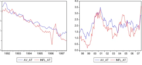
0 1 2 3 4 5 1992 1993 1994 1995 1996 1997 AV_AT INFL_AT 0.0 0.5 1.0 1.5 2.0 2.5 3.0 3.5 4.0 98 99 00 01 02 03 04 05 06 07 AV_AT INFL_AT

Figure 5: Inflation rates in Austria (INFL_AT) plotted against the average rate of inflation (AV_AT)

Austria seems to be quite well integrated with other EMU member countries. In 1992 the Austrian inflation rates were high as in the whole sample, though slightly lower than the average rates of inflation. It follows quite similar trend as the average, never drifting very far away and decreasing throughout the whole first period, usually a bit lower than the average. In the second period the Austrian inflation rates keep on following a similar trend as the sample average.

1 2 3 4 5 6 1992 1993 1994 1995 1996 1997 AV_BE INFL_BE 0.0 0.5 1.0 1.5 2.0 2.5 3.0 3.5 4.0 98 99 00 01 02 03 04 05 06 07 AV_BE INFL_BE

Figure 6: Inflation rates in Belgium (INFL_BE) plotted against the average rate of inflation (AV_AT).

From figure 5 we can see that Belgium had considerably lower inflation rates than the aver-age at the beginning of the first period, converging toward the averaver-age at the end of the pe-riod. In the second period the Belgian inflation rates seem to follow more closely to the av-erage than in the first period.

1 2 3 4 5 6 7 1992 1993 1994 1995 1996 1997 AV_DE INFL_DE 0.0 0.5 1.0 1.5 2.0 2.5 3.0 3.5 4.0 98 99 00 01 02 03 04 05 06 07 AV_DE INFL_DE

Figure 7: Inflation rates in Germany (INFLA_DE) plotted against the average rate of inflation (AV_DE).

Figure 6 shows that the German inflation rates are decreasing throughout the first period from 1992 to 1997, not showing any extreme divergence form the average and getting very close to the average in 1997. The German inflation rates seem to diverge a bit from the average at the beginning of the second period, staying below the average but still following a similar trend as the average when it comes to the movement of the inflation rates. After 2004 the German inflation rates are very close to the average and seem to follow the mean to the end of the period in 2007.

1 2 3 4 5 6 7 1992 1993 1994 1995 1996 1997 AV_ES INFL_ES 0.5 1.0 1.5 2.0 2.5 3.0 3.5 4.0 4.5 98 99 00 01 02 03 04 05 06 07 AV_ES INFL_ES

Figure 8: Inflation rates in Spain (INFL_ES) plotted against the average rate of inflation (AV_ES).

Spain had relatively high inflation rates in the early 90’s that decreased throughout the first period, managing to get inflation down to the average level in 1997. After 1997 inflation rates in Spain increased again above the average and have stayed relatively high ever since. Inflation seems to be affected by similar shocks as the rest of the EMU countries but is usually somewhat higher.

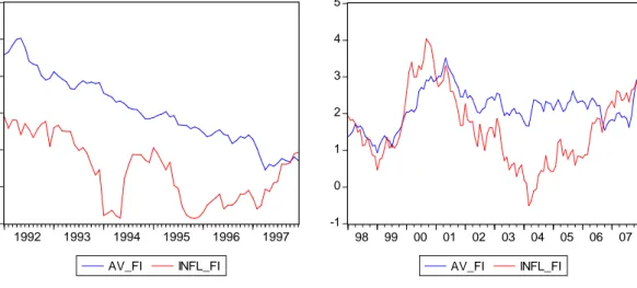
0 1 2 3 4 5 6 1992 1993 1994 1995 1996 1997 AV_FI INFL_FI -1 0 1 2 3 4 5 98 99 00 01 02 03 04 05 06 07 AV_FI INFL_FI

Figure 9: Inflation rates in Finland (INFL_FI) plotted against the average rate of inflation (AV_FI)

Inflation rates in Finland were low relative to the rest of the EMU countries at the beginning of the first period, which converged towards the average in the end of the period. Inflation rates follow the average quite closely until the year 2000 when it starts decreasing considera-bly below the average, though converging towards the average again in the 2006 and 2007.

0 1 2 3 4 5 6 1992 1993 1994 1995 1996 1997 AV_FR INFL_FR 0 1 2 3 4 98 99 00 01 02 03 04 05 06 07 AV_FR INFL_FR

Figure 10: Inflation rates in France (INFL_FR) plotted against the average rate of inflation (AV_FR)

France had relatively low inflation rates in the beginning of the 90’s, which decreased gradually throughout the whole decade, converging towards the average of the EMU in 1996 and 1997. At the beginning of the second period, the inflation rates in France seem to diverge slightly from the average, however, after 2002 they follow the average quite closely, not drifting extremely far from the average.

1 2 3 4 5 6 1992 1993 1994 1995 1996 1997 AV_IT INFL_IT 0.5 1.0 1.5 2.0 2.5 3.0 3.5 4.0 98 99 00 01 02 03 04 05 06 07 AV_IT INFL_IT

Figure 11: Inflation rates in Italy (INFLA_IT) plotted against the average rate of inflation (AV_IT)

Italy has had an unstable, high inflation economy throughout the years and very high inflation was observed in 1992. Inflation rates decreased gradually from 1992 until 1995 when Italy experienced a financial crisis which resulted in a significant increase in inflation rates. Despite of that, Italy managed to decrease its inflation rates from 5.5% in early 1996 to 1.7 % in 1997 and met the Maastricht criteria. After 1997 the Italian inflation rates have moved quite close with the average of the EMU, seemingly more integrated to the rest of the EMU when it comes to inflation rates.

1 2 3 4 5 1992 1993 1994 1995 1996 1997 AV_LU INFL_LU -2 -1 0 1 2 3 4 98 99 00 01 02 03 04 05 06 07 AV_LU INFL_LU

Figure 12: Inflation rates in Luxembourg (INFL_LU) plotted against the average rate of inflation (AV_LU)

From figure 11 we can see that Luxembourg had quite low inflation rates relative to the av-erage and decreasing throughout the period 1992 to 1997. By the end of the period, the tion rates were slightly lower than the average but quite close. In the later period, the infla-tion rates in Luxembourg stayed quite close to the average and followed a similar trend throughout the whole period.

1 2 3 4 5 1992 1993 1994 1995 1996 1997 AV_NL INFL_NL 0 1 2 3 4 5 98 99 00 01 02 03 04 05 06 07 AV_NL INFL_NL

Figure 13: Inflation rates in the Netherlands (INFL_NL), plotted against the average rate of inflation (AV_NL)

Inflation rates in the Netherlands showed decreasing trend throughout most of the period 1992 to 1997 and staying lower than the average until the end of the period when it increased a bit over the average. After 1998, inflation rates in the Netherlands started increasing and were considerably higher than the average during 2001 and 2002. After that they decreased significantly and have stayed below the average since 2004

1 2 3 4 5 6 7 8 9 10 1992 1993 1994 1995 1996 1997 AV_PT INFL_PT 0 1 2 3 4 5 6 98 99 00 01 02 03 04 05 06 07 AV_PT INFL_PT

Figure 14: Inflation rates in Portugal (INFL_PT), plotted against the average rate of inflation (AV_PT).

In 1992 the inflation rates in Portugal were the highest of all the 11 original EMU countries, peaking at just under 10% in 1992. During the period 1992 to 1997 the inflation rates decreased gradually and converging towards the EMU average, getting even lower for some time in 1997. However, after 1998 the inflation rates in Portugal increased sharply and started diverging from the EMU average again and stayed considerably higher throughout the period 1998 to 2007, though converging somewhat at the end of the period.

From figures 5 to 14 we can see that inflation rates in the 10 countries were decreasing throughout the period 1992 to 1997 and in most cases converging towards the average at the end of the period, with the exception of Austria in which case the inflation rates seem to follow quit closely throughout both of the periods analysed. However, in the period 1998 to 2007 it is hard to see a clear patter from the figures, where in some cases the countries seem to follow the average more closely then in the earlier period (such as Belgium, Italy and Luxembourg). Furthermore, we can see in the end of the period 1998 to 2007 that inflation rates start following the average of the remaining countries more closely in all of the countries. A possible reason for this pattern could be that a price convergence is a factor in the inflation rate divergence process as theory suggests and that price convergence has slowed down at the end of the period. However, we will leave that question for future research.

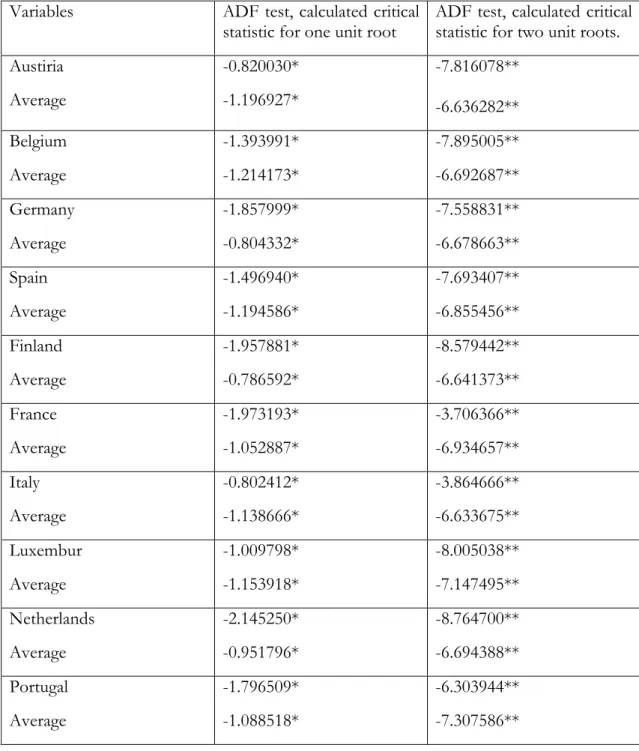
For our purpose to determine whether the inflation rates among the European countries are cointegrated or not the ADF test, Engle-Granger cointegration test and Johansen cointegration test were used9_.

Table A1 in the appendix shows the results of the unit root tests for the period 1992 to 1997. We concluded with a 95% significance level, that all the countries in the sample contained one unit root, that is, were integrated of order one. Moreover, the unit root tests for the average measures also were integrated of order one, making it relevant to test for cointegration for all the countries. Despite the fact that the graphical analysis indicate for all the sample countries that the inflation rates are converging, we could only reject the null