Stock Price Valuation : A Case study in Dividend Discount models & Free Cash Flow to Equity models

Stock Price Valuation

A Case study in Dividend Discount models & Free Cash Flow to Equity models

Master‟s thesis within Finance

Authors: Anders Karlsson Niklas Josefsson

Master‟s Thesis within Finance

Title: Stock Price Valuation

Authors: Anders Karlsson and Niklas Josefsson

Tutor: Urban Österlund

Date: 2011-09-30

Subject terms: Valuation of stock price, Valuation Models, Case Study

Abstract

Purpose The purpose of this study is to investigate how much the result will differ when calculating stock price for firms when using DDM model compared to FCFE. We will also like to find out if there is a specific payout ratio where DDM works better than FCFE and how accurate are DDM and FCFE model when used to value different companies.

Method This is a qualitative study where the collection of our empirical data will be retrieved from the theoretical framework and precious re-search. In the stock price valuation area there are many sources of information, however the focus to gain information in the subject where on non-fiction books. We also looked at suggested reading and reference lists from relevant working papers, books and articles.

Empirical Findings In this section we present our findings from the valuation of the 10

companies. We analyze and present our data together with assump-tions made for every company. After this an extended analysis is presented, the purpose of this section is to get a better understand-ing from our results in the empirical findunderstand-ings and to analyze the data even more.

Conclusion We concluded that the results differ a lot from use of the two dif-ferent valuations models and that they work better in difdif-ferent situa-tions. Also, none of the two models are very accurate when valuat-ing a specific company, there are too many unknown parameters that can affect the result. However, in the research we saw that there is a tendency for FCFE model to work better with companies with low dividend pay-out ratio and that DDM works better on compa-nies with high divided pay-out ratio.

Table of Contents

1

Introduction ... 1

2

Theoretical Framework ... 6

2.1 The Efficient Market Hypothesis ... 6

2.1.1 Different types of Efficiency ... 8

2.2 Discounted Cash Flow (DCF) ... 9

2.3 Dividend Discount Model (DDM) ... 10

2.3.1 Price of stock with zero growth dividends ... 11

2.3.2 Price of stock with constant growth dividends (Gordon Growth Model) ... 11

2.3.3 Price of stock at time N with constant growth dividends (Terminal Value) ... 12

2.3.4 Two-stage Dividend Discount Model ... 13

2.3.5 Three-stage Dividends Discount Model ... 14

2.3.6 Modified Dividend Discount Model ... 15

2.4 Equity Valuation ... 16

2.5 Free Cash Flow to Equity Discount Models ... 16

2.5.1 Cash to stockholders to FCFE ratio ... 16

2.5.2 Constant Growth FCFE Model ... 17

2.5.3 Two-stage FCFE Model ... 17

2.5.4 Three-stage FCFE Model (E Model) ... 18

2.6 Future Growth ... 19

2.7 Previous Research ... 21

3

Methodology ... 24

3.1 Methodological Approach ... 24

3.2 Outline of the Study ... 24

3.3 The research process of the thesis ... 25

3.4 Inductive vs. Deductive ... 26

3.5 Qualitative vs. Quantitative ... 27

3.6 Data Search ... 28

3.7 Criticism of the Sources ... 29

3.8 The Approach and Structure of the Thesis ... 29

3.9 Validity and Reliability ... 31

3.9.1 Validity ... 31

3.9.2 Reliability ... 32

3.10 Criticism of Method ... 32

4

Empirical findings and Analysis ... 34

4.1 Alfa Laval ... 34

4.1.1 Assumptions ... 34

4.1.2 Two-stage DDM ... 35

4.2.1 Assumptions ... 37 4.2.2 Two-stage DDM ... 38 4.2.3 Two-stage FCFE ... 38 4.3 Atlas Copco ... 39 4.3.1 Assumptions ... 39 4.3.2 Two-stage DDM ... 40 4.3.3 Two-stage FCFE ... 41 4.4 Axfood ... 41 4.4.1 Assumptions ... 41 4.4.2 3-stage DDM... 42 4.4.3 3-stage FCFE ... 42 4.5 Boliden ... 43 4.5.1 Assumptions ... 43 4.5.2 Two-Stage DDM ... 44 4.5.3 Two-Stage FCFE ... 44 4.6 Ericsson ... 45 4.6.1 Assumptions ... 45 4.6.2 Two-stage DDM ... 46 4.6.3 Two-stage FCFE ... 47 4.7 H&M AB ... 47 4.7.1 Assumptions ... 48 4.7.2 Two-stage DDM ... 49 4.7.3 Two-stage FCFE ... 49 4.8 Holmen ... 50 4.8.1 Assumptions ... 50

4.8.2 Gordon Growth Model ... 51

4.8.3 FCFE ... 52

4.9 TeliaSonera ... 52

4.9.1 Assumptions ... 52

4.9.2 Gordon Growth Model ... 53

4.9.3 FCFE ... 54

4.10 Volvo ... 54

4.10.1Assumptions ... 55

4.10.2Gordon Growth Model ... 55

4.10.3FCFE ... 56

5

Extended Analysis ... 57

6

Conclusion ... 60

7

Discussion and Reflections ... 62

7.1 Future Studies ... 62

8

References ... 63

Appendices ... 68

Appendix 6 ... 71 Appendix 7 ... 72 Appendix 8 ... 72 Appendix 9 ... 73 Appendix 10 ... 74 Appendix 11 ... 74 Appendix 12 ... 75 Appendix 13 ... 75 Appendix 14 ... 75 Appendix 15 ... 76 Appendix 16 ... 77 Appendix 17 ... 78 Appendix 18 ... 78 Appendix 19 ... 79 Appendix 20 ... 79 Appendix 21 ... 80 Appendix 22 ... 81 Appendix 23 ... 82 Appendix 24 ... 82 Appendix 25 ... 83 Appendix 26 ... 83 Appendix 27 ... 84 Appendix 28 ... 85 Appendix 29 ... 86 Appendix 30 ... 86 Appendix 31 ... 87 Appendix 32 ... 87 Appendix 33 ... 88 Appendix 34 ... 89 Appendix 35 ... 90 Appendix 36 ... 90 Appendix 37 ... 91 Appendix 38 ... 91 Appendix 39 ... 92 Appendix 40 ... 93 Appendix 41 ... 94 Appendix 42 ... 94 Appendix 43 ... 95 Appendix 44 ... 95 Appendix 45 ... 96 Appendix 46 ... 97 Appendix 47 ... 98 Appendix 48 ... 98 Appendix 49 ... 99 Appendix 50 ... 99 Appendix 51 ... 100 Appendix 52 ... 101 Appendix 53 ... 101 Appendix 54 ... 102

Appendix 55 ... 102 Appendix 56 ... 103 Appendix 57 ... 103 Appendix 58 ... 104 Appendix 59 ... 104 Appendix 60 ... 105 Appendix 61 ... 105

Figures And Tables

Figure 2 Market Efficency ... 6

Figure 3 Relationship among three different information sets ... 8

Figure 4 Future Growth ... 10

Figure 5 The research process of the thesis ... 25

Figure 6 Alfa Laval, Stock price valuation ... 36

Figure 7 Assa Abloy, Stock price valuation ... 38

Figure 8 Atlas Copco, Stock price valuation ... 40

Figure 9 Axfood, Stock price valuation ... 42

Figure 10 Boliden, Stock price valuation ... 44

Figure 11 Ericsson, Stock price valuation ... 46

Figure 12 H&M, Stock price valuation ... 48

Figure 13 Holmen, Stock price valuation ... 50

Figure 14 TeliaSonera, Stock price valuation ... 53

Figure 15 Volvo, Stock price valuation ... 55

Figure 16 Stock Prices ... 58

Table 1 Sources used in the Study ... 29

1

Introduction

This chapter is an introduction to the thesis. First, a background about the subject is given followed by a problem discussion with our main questions leading to the purpose of the thesis.

1.1

Background

Valuation is the process of forecasting the present value of the expected payoffs to share-holders. According to Lee, C.M (1999) valuation models are merely „pro form accounting systems‟ that constitute the tools for articulating the assessment of future events typically in terms of accounting constructs. Barker, R (2001) argues that a good understanding of valu-ation methods requires two main things, the first is an analytical review of the models. The second is an evaluation of the data that are available for use of these models. It is because of this there is a significant relationship between the choice of valuation models and the available data.

A valuation model is a mechanism that converts a set of forecasts of (or observations on) a series of company and economic variables into a forecast of market value for the compa-ny‟s stock. The valuation model can be considered a formalization of the relationship that is expected to exist between a set of corporate and economic factors and the market‟s valu-ation of these factors (Elton, Gruber, Brown, & Goetzmann 2011).

The models that we use in valuation may be quantitative, but the inputs leave plenty of room for subjective judgments. Thus, the final value that we obtain from these models is colored by the bias that we bring into the process. In fact, in many valuations, the price gets set first and the valuation follows (Damodaran 2002)

Valuation models has been an essential part in the study of finance for quite some time, and a continuous discussion is going on concerning the accuracy of different valuation models and how efficient they are in predicting future firm value.

The search for the “correct” way to value common stocks, or even one that works, has oc-cupied a huge amount of effort over a long period of time. Attempts have ranged from simple mechanical techniques for picking winners to hypotheses about the broad influences affecting stock prices (Elton, Gruber, Brown, & Goetzmann 2011)

Casti. J (1998) mentions the simple observation, that there is no single best way to process information. This led Arthur and Holland to the not-very-surprising conclusion that

deduc-tive methods for forecasting prices are, at best, an academic fiction. As soon as you admit the possibility that not all traders in the market arrive at their forecast in the same way (more about this in the section about market efficiency), the deductive approach of classical finance theory begins to break down. So a trader must make assumptions about how other investors form expectations and how they behave. He or she must try to “psyche out” the market. But this leads to a world of subjective beliefs and to beliefs about those beliefs. In short, it leads to a world of induction rather than deduction.

Sweden and most of the world for that matter has recently been in a deep financial reces-sion, which most people would argue, in the writing this (spring of 2011) is over even though some still argue for the chance of a “double dip” and the chance of heading into a new recession. During the financial crises the discussion of the accuracy of financial mod-els have started to increase again and with questions like; how can we say that one valuation models work better than another, when most of the models use historic data together with biased information such as, among others human interpretations, rumors about the corpo-ration, and other external information.

Further it is important to emphasize that a valuation is not timeless, quite the opposite in fact, a valuation is as mentioned above a mechanism for turning a set of historical or pre-dicted variables to determined a possible present values for the corporation‟s stock. Va-riables as might be interpret by the name can vary, and as the inputs of the model changes the outcome that is predicted with the model will also change. This is why as mentioned the earlier after the latest financial crises in Sweden more people have come to criticize the value of valuation models.

As mentioned above firm valuation is a quantitative valuation model and from that it might be logical argue that more inputs (variables) would lead to a better model with a prediction closer to the true value, but basic statistic tells us that in fact the opposite might be true. As more variables are added into a model the risk for input errors might increase, and at some point the cost will overweight the benefits of adding a variable. The problems with more complex models amplifies as the users start to not understand the importance of each variable, at some point they can become so complex that they become „black boxes‟ where analysts feed in numbers into one end and valuations emerge from the other. All too often the blame gets attached to the model rather than the analyst when a valuation fails, Damo-daran (2002).

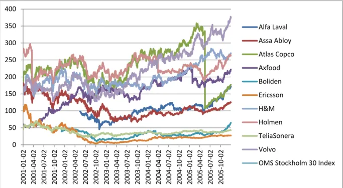
Figure 1 Stock Prices

As seen in the graph above stock price varies a lot over time and both changes from day to day to a yearly basis might be difficult to value. When using valuations as dividend discount model (DDM) and free cash flow to equity (FCFE) it is important to realize that it is usual-ly a long term prediction for the corporation where market fluctuations would equal out. Both of this models use all future cash flows until perpetuity and then it is discounted back to today or a time of preference that could be compared with the actual price to see if the stock is undervalued or overvalued.

In the graph above you can also see that the different companies that we decided to value tend to move in somewhat the same direction with some companies being less sensitive to the market and some more. In the graph above we also see the effect of the stock split that Atlas Copco did during 2005.

1.2

Problem Discussion

The key to successfully investing in different assets, stocks and firms lies in understanding that every asset, financial as well as real has a value. A real asset is an assets used to produce goods and services, financial assets are assets such as bonds and stocks. Any asset can be valued but some are easier to value than others, and depending on valuation method you

0 50 100 150 200 250 300 350 400 2001 -01 -02 2001 -04 -02 2001 -07 -02 2001 -10 -02 2002 -01 -02 2002 -04 -02 2002 -07 -02 2002 -10 -02 2003 -01 -02 2003 -04 -02 2003 -07 -02 2003 -10 -02 2004 -01 -02 2004 -04 -02 2004 -07 -02 2004 -10 -02 2005 -01 -02 2005 -04 -02 2005 -07 -02 2005 -10 -02 Alfa Laval Assa Abloy Atlas Copco Axfood Boliden Ericsson H&M Holmen TeliaSonera Volvo

There are a various number of different valuation methods to choose from when doing a forecast of a firm, you have both sophisticated and unsophisticated valuation methods. So-phisticated methods are based on net present value (NPV) of the financial performance of multiple future periods. Unsophisticated valuation methods are simpler methods based on the multiple of a single period‟s performance measure to price relative to the same measure for comparable firms (Flöstrand, P. 2006). Our use of models in this study will involve models such as Dividend Discount Model (DDM) with different growth stages and Free Cash Flow to Equity (FCFE). The dividend discount model is based upon the premise that the only cashflows received by stockholders is dividends. According to Damodaran, A (2002) even if we use the modified version of the model and treat stock buybacks as divi-dends there is a chance we misvalue firms that consistently return less or more than they can afford to their stockholders. In contrast the FCFE model uses a more expansive defini-tion of cashflows to equity as the cashflows left over after meeting all financial obligadefini-tions, including debt payments, and after covering capital expenditure and working capital needs. These differences in the models lead us to following questions:

 How will the result differ when calculating stock price for firms when using DDM compared to FCFE?

 Is there a specific payout ratio where DDM works better than FCFE?

 How accurate are DDM and FCFE model when used to value different companies?

1.3

Purpose

The purpose of this study is to get an understating of how the result differs when calculat-ing stock price for firms when uscalculat-ing DDM model compared to FCFE. We will also like to find out if there is a specific payout ratio where DDM works better than FCFE and how accurate are DDM and FCFE model when used to value different companies.

1.4

Delimitation

Limitations are necessary and important in order to keep a high quality throughout the en-tire thesis. Our focus will be on companies which pay out dividends, this is important since dividends are a crucial part when calculating firm‟s stock price. Our choice of models is Dividend Discount Model and Free Cash Flow to Equity since these models are most

ap-propriate when dealing with dividends. We also decided to limit our search of companies only to large cap on the Swedish stock exchange market. The number of companies we will evaluate will be 10, we believe that this will be enough in order to get a fair result.

Furthermore, the thesis will focus on the recommendations of the literature, therefore the other areas of the valuation process will not be carried out by thorough analysis, rather as-sumptions and simplifications will be made. When choosing between stock A, B and C we only focus on the stock that is most traded.

2

Theoretical Framework

This Chapter explains the necessary theories used to answer the problem. First, the theory of efficient mar-kets is explained. Second the necessary investment models are explained.

2.1

The Efficient Market Hypothesis

When someone refers to efficient capital markets, they mean that security prices fully re-flect all available information (Elton, Gruber, Brown, & Goetzmann 2011). If this where to be hold true in the financial market there would be no use of financial valuation models to find possible mispriced securities, since all securities are valued and traded at the price re-flected by all available information.

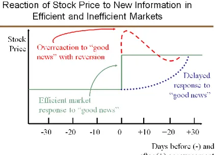
Figure 2. Ross, Westerfield and Jaffe, 2008

For the hypothesis that all security prices fully reflect all available information should hold true, a necessary condition is that the cost of acquiring information and trading is zero (El-ton, Gruber, Brown, & Goetzmann 2011). This clearly is not the case in the markets today even though there is and has been a clear decrease in cost both of information and trading. Figure 2 above describes the reaction to new good information in an efficient market and in an inefficient market. In an efficient market the reaction to new news is instant and no over- or under-reaction exist whatsoever. In an inefficient market however there would be two different possible responses to the new news, either the market can slowly adjust to the information or an overreaction occurs and then it will take some time for the market to ad-just to the “right price”.

As mentioned earlier a necessary condition for market efficiency to hold true is that the cost of acquire information and trading is zero. Ross, Westerfield and Jaffe (2008) also mentions three other conditions that cause market efficiency: Rationality, independent dev-iations from rationality and arbitrage.

Rationality is important since when new information is released in the marketplace, all

in-vestors will adjust their estimates of stock prices in a rational way. Price of a stock will also rise immediately because rational investors would see no reason to wait before trading at a new price. Theory and reality in this case goes different ways, where the theory sounds good, people tend not to act rational in all situations hence it might be too much to argue that all investors should behave rationally. The market would however still be efficient if the following scenario holds (Ross, Westerfield and Jaffe 2008).

Independent Deviations from Rationality would tell us that if as many individuals were

irrationally optimistic as were irrationally pessimistic prices would likely rise in a manner consistent with market efficiency. Deviations from rationality could for example happen when new information released are not clear and leaves some room for interpretation and emotions for investors. Some investors could have some positive emotions towards the corporation and its news while others have the opposite emotions. As long as the irratio-nalities offset each other we could have a market that is efficient even though most inves-tors would be classified as less than fully rational. It is however arguably not realistic to as-sume that irrationalities offset each other immediately, instead it might be more rational to argue that if there is “good” news most investors would get swept away and overreact to the news just as figure 1 above shows. Even in the case of independent deviations from ra-tionality there is an assumption that will produce market efficiency (Ross, Westerfield and Jaffe 2008).

Arbitrage, assumes that there are two types of people in the market, irrational amateurs

and the rational professionals. Amateurs would from time to time make irrational decisions and think that a stock is undervalued and sometimes the opposite. When the behavior of the amateurs does not cancel out and create a efficient market, the behavior of professional get important. Professionals are methodical and rational, and with thoroughly studies of the companies they find objective evidence of the true value of the stock and act thereafter pushing the prices to the true value and create an efficient market as long as the arbitrage of professionals dominates the speculation of amateurs (Ross, Westerfield and Jaffe 2008).

2.1.1 Different types of Efficiency

Up to this point we have been discussing market efficiency, as being a market that directly without any delay responds to all new information, this is considered to be a strong form of market efficiency. Now two new types of efficiency are introduced, the weak and the semistrong form of efficiency.

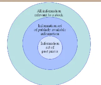
The weak form of market efficiency is when security prices already include all information

found in past prices and volume. If this holds true there would be no reason to use tech-nical analysis to find deviation in stock price.

Weak form efficiency is often represented mathematically as:

The random term in the formula above is there to cover new information that we at time t do not know. The random error is not predictable from earlier data hence the stock price will follow a random walk ( Ross, Westerfield and Jaffe 2008).

The semistrong form as seen in the second to largest circle above hold a stronger

defini-tion to what is an efficient market. In the semistrong form of an efficient market all infor-mation set by past prices and volume as well as all other public inforinfor-mation has to be in-cluded in the stock price of any given firm for it to be efficient.

The strong form is the hardest way to look at a efficient market and for a market to be

ef-ficient under the strong form the same as in a semistrong form has to be true and also all private information must be reflected in the stock price even if just one person have the in-formation.

2.2

Discounted Cash Flow (DCF)

Discounted cash flow valuation is one of our main ways of approaching valuations, and ac-cording to (Damodaran, A. 2002, p. 14) DCF is the foundation on which all other ap-proaches are built upon. In order to do relative valuation correctly we need to understand the fundamentals of discounted cash flows valuation. Moreover discounted cash flow models are based on the concept that the value of a share of stock is equal to the Present Value (PV) of the cash flow that the stockholders expects to receive from it. (Elton, E, Gruber, M, Brown, S, Goetzmann, W. 2011)

Discounted cash flow valuation is a method of valuing a project, company, or asset using the concepts of the time value of money. All future cash flows are estimated and discounted to give their present values (PVs) – the sum of all future cash flows, both incoming and outgoing, is the net present value (NPV), which is taken as the value or price of the cash flows in question. This section will present a result of the firm‟s present value as well as the value of the stock

Basis for discounted cash flow valuation has its foundation in the net present value (NPV), where the value of any asset is present value of expected future cash flows that the asset generates.

Where,

n = Life of the asset = Cash flow in period t

r = Discount rate reflecting the riskiness of the estimated cash flows

Obviously the cash flows will vary from asset to asset, the discount rate will be a function of the riskiness of the estimated cash flows, the riskier assets the higher rates and vice versa for safer projects. (Damodaran, A. 2002, p. 15)

According to Neale, B & McElroy, (2004, p 314-315) the main problems with the DCF ap-proach centre on the key variables in the model. Can future investment levels be accurately projected? How can we measure the discount rate? Over what time should we assess value? Should we accept the current earning figure? These are all questions that are key in under-standing valuation.

2.3

Dividend Discount Model (DDM)

There are numbers of different discounted cash flow models one can use, however in this paper we will focus on Equity Valuation using Dividend Discount Model (DDM) and Free Cash Flow to Equity (FCFE), since we are only interested in valuing the stock price. DDM is a method for valuing the price of a stock for a company which pays out dividends, as-suming that the price of a stock is equivalent to the sum of all of its future dividend pay-ments discounted to the present value. Within this model you can use a set of different ap-proaches such as;

 Price of stock with zero growth dividends

 Price of stock with constant growth dividends (Gordon Growth Model)

 Price of stock at time N with constant growth dividends (Terminal Value)

2.3.1 Price of stock with zero growth dividends

Since the zero growth model assumes that the dividend always stay the same, the stock price would in that case be equal to the annual dividends divided by the Rate of Return (ROR). The stockholders can therefore expect that future earnings will be flat and there will not be any further increase in the dividends payout. In order to calculate the value of the stock for we use the formula:

Where,

= Dividend

= Required rate of return for equity investors g = Dividend Growth Rate

2.3.2 Price of stock with constant growth dividends (Gordon Growth

Model)

Using the Dividend Discount Model to value the price of the stock, we sum all the compa-ny's future dividends, which in this case is assuming to grow at a constant rate. This model works best when valuating stocks for established companies, meaning that they should have increased the dividend steadily over the years. Although the annual increase is not al-ways the same Gordon Growth Model can be used to approximate an intrinsic value of the stock. This is the least sophisticated of the DDM, but there are still some important aspects that is needed to be considered, as mentioned before the growth has to be stable which could be difficult to determined for some companies. Important is also to realize the im-portance of growth in all DDM‟s, since small variations in growth will make a large impact on the value.

Where,

= Required rate of return for equity investors g = Dividend Growth Rate

Further it is important to recognize that growth cannot exceed the market capitalization rate. If dividends were expected to grow forever at a rate faster than k, the value of the stock would be infinite (Bodie, Z, Kane, A, Marcus, A. 2008). It might be nonsensical, but, in reality this occurs often for companies in the real market especially for firms that are in a period of high growth, usually this growth settles down after a period of time to a more normalized growth, more about this in chapter 2.6. When the company that is being valued is experiencing a growth rate higher than the discount rate there are two ways to handle it so the DDM would be effective. First, the growth could be considered as a long term aver-age or a normal growth rate. This is a far from a satisfactory way to handle the problem, since the rapid growth often occurs the early stage of the life cycle and the value computed when using a average growth will highly underestimate the near future dividends. Alterna-tively, the growth could be segmented into different stages of the financial cycle, and each of these stages could be valued separately, this is being explained more detail later (Pike, R & Neale, B. 2003).

2.3.3 Price of stock at time N with constant growth dividends (Ter-minal Value)

According to Damodaran, A (2002) many companies grow very rapidly in its first few years and then subsequently settling down to a constant growth rate. In this case we have to con-sider both the initial hyper growth stage and then the subsequent constant growth stage in order to value the price of the stock of a company. The constant growth stage is similar to the Gordon growth model where we value the price of a constant growth stock.

Where,

= Price (terminal value) at end of year n = Expected dividends per share in year n (

= Steady state growth rate forever after year n

2.3.4 Two-stage Dividend Discount Model

As mentioned above companies tend to initially grow very rapidly in its first few years and then subsequently settling down to a constant growth rate, however to value the stock price of a company with non-constant growth increases the difficulty, one way is to assume that the company instead have a two stage growth.

Where,

= Stock price at time=0

= Expected dividends per share in year t

= Cost of Equity (hg: High Growth period; st: Stable growth period) = Price (terminal value) at end of year n

g = Extraordinary growth rate for the first n years = Steady state growth rate forever after year n

Two-stage DDM is better suited than Gordon growth model for companies that has not yet reached a state of steady growth, but it far from a perfect way to value stock price. First there are now two different growths to be considered, we have the high growth stage which could be difficult to determine since the growth can vary heavily from year to year. Then the constant growth rate has to be determined for the perpetuity. Second, you have to determine for how many years the high-growth phase will continue before the firm will enter into a steady state. Third the two-stage DDM implies that the growth would abruptly end and that the company would then immediately enter a constant growth state, more rea-listic would be that this transition would happen over a longer period of time.

2.3.5 Three-stage Dividends Discount Model

When a firm is in a three stage it is first assumed to be in an extraordinary growth phase currently, this extraordinary growth is expected to last for an initial period that has to speci-fied. After this the growth rate declines linearly over the transition period to a stable growth rate. Here we use the following formula:

Where,

= Stock price at time=0

= Expected dividends per share in year t

= Growth rate in high growth phase (lasts for n1 periods) = Steady state growth rate forever after year n

= Payout ratio in high growth phase = Payout ratio in stable growth phase

= Cost of Equity (hg: High Growth phase; t: transition phase; st: Stable growth phase)

Three-stage DDM is superior to the two-stage DDM in the way that there is a transaction phase where you can account for the time it takes to go from a initial high growth phase to a normal growth. With the extra input there is also some negative aspects, as mentioned before it‟s difficult to determined for how long the initial high grow phase will continue this is still a problem in the three-stage model but know there is also the aspect of deter-mine how long the decline from high- to low-growth will take but also how the decline will occur. The decline can occur in a number of ways with the easiest to use arguably being a straight line decline. The difficulties in determine the length of the high growth phase and the transaction period together with determining in what whey de decline will happen af-fects the accuracy of the prediction. A decision has to be made whether the addition will add to get a more precise value or in fact decline the accuracy of the prediction.

A problem with all dividend-based valuations are that they apply the assumption that there is a informative relationship between current dividends and future dividends, this might hold true in most cases, but in theory it might not. The biggest fundamental problem with the dividend-based valuation however might be that they do not address the determinants of dividend growth. Dividend-based models have no explanation between current divi-dends and future dividivi-dends, Barker, R (2001).

2.3.6 Modified Dividend Discount Model

When using DDM your focus is strictly on dividends paid as the only cash returned to stockholders, this exposes us to the risk that we might be missing significant cash returned to stockholders in the form of stock buybacks Damodaran, A (2002). The simplest way to incorporate stock buybacks into a dividend discount model is to add them on the dividends and compute a modified payout ratio:

Modified dividend payout ratio =

It is important to have in mind that the he resulting ratio for any one year can be skewed by the fact that buybacks unlike dividends are smoothed out, a much better estimate of the modified payout is therefore by looking at the average value over a period. In addition, firms may sometimes buy back stocks as a way of increasing financial leverage, we could adjust for this by netting out new debt issues.

Modified dividend payout ratio =

By adjusting the payout ratio to include stock buybacks will have effects on the estimated growth and terminal value. Damodaran, A (2002)

By using following formula you calculate the modified growth rate: Modified growth rate = (1-Modified payout ratio) * Return on equity

2.4

Equity Valuation

The value of equity is obtained by discounting expected cash flows to equity such as the re-sidual cash flows after meeting all expenses, reinvestment need, tax obligation and net payments, at the cost of equity i.e. the rate of return (ROR) required by equity investors in the firm. (Damodaran, A. 2002, p. 17)

Where,

= Expeted Cash flow to Equity in period t = Cost of Equity

2.5

Free Cash Flow to Equity Discount Models

2.5.1 Cash to stockholders to FCFE ratio

The Cash to stockholders to FCFE ratio shows how much of the cash available to be paid out to stockholders in the firm that is actually paid out to them, in form of dividends and stock repurchases. (Damodaran, A. 2002)

A value of 1 would imply that the firm is returning all the available cash after meeting its expenses to the owners. Therefore a value below 1 means that the firm is not paying out all that they can afford, and keep some of it in the firm, reasons for this could be amongst others to reinvest it in positive net present value project, increase cash balance and future

acquisitions of firms. If the firm pays out more than they can afford the value would be above 1, this is usually not an option in the long-run and it means that the firm is taking the extra money from existing cash balances or by issuing new securities.

2.5.2 Constant Growth FCFE Model

The constant growth model is used to value firms that are only growing at a stable rate. This model is very similar to the Gordon growth model, with the difference that FCFE is used instead of dividends. Important to this model is that the growth rate is reasonable since “it continues forever”. The growth rate should be set to the nominal growth rate in the economy in which the company operates or close to this if it could be justified. If a constant growth FCFE model is chosen, it is also implied that the firm is a stable firm and that it has the characteristics of a stable firm. (Damodaran, A. 2002)

Where,

= Value of stock today = Expected FCFE next year

= Cost of Equity

= Growth rate in FCFE for the firm forever

2.5.3 Two-stage FCFE Model

Two-stage FCFE model is just as two-stage DDM, used to value a firm that first have a high growth that after some years will turn in to a stable growth. Two-stage models has an advantage to three-stage models in that it is not so sophisticated and you don‟t have to de-termine in what way the change from high growth to low-growth occurs. This on the other hand also makes it less true in the real world, since a firm will not go from high to low growth immediately, this would happen over time and you are able to show this decline better in a three-stage model.

Where, Where,

= Free cash flow to equity in year t

= Price at the end of the extraordinary growth period

= Cost of equity high growth phase = Cost of equity stable growth

= Growth rate in FCFE for the firm forever

2.5.4 Three-stage FCFE Model (E Model)

As mentioned earlier a three-stage model has three separate phases, first there is the high growth phase where the firm experience abnormal growth. Second we have the change from high growth to normal growth, something called the transition stage. Last is the normal or low growth.

Where, Where,

= Value of stock today

= Free cash flow to equity in year t = Cost of Equity

= Cost of equity stable growth

= End of initial high-growth period = End of transition period

2.6

Future Growth

When predicting future growth for a corporation it important to realize in what stage of the life-cycle the corporation is. As firms grow larger the cash flow and risk exposure is rela-tively predictable which makes valuation easier. Depending on what stage the company be-longs to, the company is faced with different choices. Damodaran (2001) mentions that most usual is to divide the life-cycle into five different stages:

1. Start-up: This is the first stage after a firm is started, usually a firm in this stage is funded by owners equity or by loans. Under this stage a firm is trying to build up a client base and get established.

2. Expansion: When a company has managed to build up a client base and established a presence in the market, the funding needs to increase to be able to expand the company further. Firms in this stage are unlikely to generate high internal cash flows but at the same time investment needs are likely to be high. To fund the in-vestment needs firms are likely to turn to private equity or venture capital, some might even go public to raise the extra capital.

3. High growth: As firms transition into publicly traded firms the financial choices in-creases. In this stage a firms revenues are growing rapidly but earnings are likely to lag behind, and internal cash flow lags behind the reinvestment needs. Most com-monly publicly traded firm will use equity issues to raise the capital needed while when using debt as financing they will most likely use convertible debt to raise the capital.

4. Mature growth: When corporations mature. The growth will start to level off, when this happen the earnings and cash flows that has been lagging behind will rapidly increase and the need to invest in new projects will decrease accordingly. During this period most corporations also change their financing from mainly a equity based financing to a debt financing to fund future projects.

5. Decline: The last stage in the life cycle is the decline. This means that both revenues and earnings will start to decline, as the business mature and new competitors take market share from them. Their existing investments will continue to produce cash

companies will probably start to retire debt and buy back stock, in a way the com-pany has started to liquidate itself.

Figure 4, Future Growth

Important to realize is that not all companies go through all five stages and the choices are not the same for all of them, neither are the opportunities. A major part of the companies that are started never makes it past the first stage and are closed down, also many compa-nies continue as small compacompa-nies without or with small expansion potential. Not all com-panies choose to go public in fact many choose to be private and can still continue to grow at a healthy rate, Damodaran, A (2001).

One way for growth in dividends is to increase the equity from shareholders, then the growth simply arises from the fact a larger amount of capital is likely to generate a larger income stream. When discussing dividends what is usually more interesting is dividends per share, and to increase dividends per share a corporation has to have a rate of return on new capital that exceeds the rate of return on already existing capital. A second options to in-crease dividends per share is when a company earns a positive return on capital it has the choice to either paying the profit back to the shareholders, which could be by either by div-idends or stock-buy-backs, or it can choose to reinvest the earnings for future projects, Barker, R (2001).

So for a sustainable growth in dividends, the company needs to have a positive return on shareholders‟ capital and also that shareholders capital will be able to grow either be rein-vestment of profits or by new inrein-vestments, Barker, R (2001)

2.7

Previous Research

There are quite a lot of other studies that have been conducted on firm valuation, some dif-ferent from others when conducting valuations. They investigate, compare and contrast, which models analysts use and how these analysts look at the models, see Absiye and Di-king (2001) and Carlsson (2000). Others focus on how one, or a couple of the valuation models are constructed, see for example Eixmann (2000)

There are many scientific studies conducted on forecasting, but most of these are not in the context of firm or stock valuation. They are usually focused on macroeconomic forecasting or short term forecasting where mostly sales volume and similar quantities are forecasted. Textbooks that mention different approaches to forecasting sales are i.e. Copeland et al (2000)

In the area of equity analysis, research in finance has not been very successful. Equity anal-ysis or fundamental analanal-ysis was once the mainstream of finance. But, while enormous steps have been taken in pricing derivatives on equity, techniques to value equities have not advanced much beyond applying the dividend discount model. Penman, S.H and Nissim, D. (2001) So-called asset pricing models, like the Capital Asset Pricing Model have been developed but these are models of risk and expected return, not models that instruct how to value equities.

Traditional fundamental analysis was very much grounded in the financial statements, Gra-ham, Dodd And Cottle‟s (1962) and financial statement measures were linked to equity value in an ad hoc way, so little guidance was given for understanding the implications of i.e. a particular ratio, a profit margin or an inventory turnover for equity value. Nor was comprehensive scheme advanced for identifying, analyzing and summarizing financial statement information in order to draw a conclusion as to what the statements as a whole really say about the equity value. Penman, S.H and Nissim, D. (2001, p 110)

A considerable amount of accounting research in the years since Graham, Dodd and Cottle has been involved in discovering how financial statements inform about equity value. Ac-cording to Nissim and Penman the whole endeavor of capital market research deals with the information content of financial statements for determining stock prices. There are a lot of papers on this subject such as Lipe (1986), Ou and Penman (1989), Ou (1990) Lev

and Thiagarajan (1993) and Fairfield, Sweeney and Yohn (1996) that examine the role of particular financial statement components and ratios in forecasting stock prices. However Nissim and Penman argue that it is fair to say that the research has not been conducted with much structure, nor has it produced many innovations for practice. It is important to mention that empirical correlations in these papers have been documented but the research has not produced convincing financial statement analysis for equity valuation.

The dividend discount model attraction is its simplicity and its logic, however there are many analysts who view its results with some suspicion because of the limitations that they believe it possess. According to Damodaran (2002) some researcher claim that dividend discount model is not really useful in valuation, expect for a limited number of stable, high-dividend paying stocks.

A standard critique of the dividend discount model is also that it provides a too conserva-tive estimate of the value. This is based on the notion that the value is determined by more than the present value of expected dividends. It is argued by researchers that the DDM does not reflect the value of unutilized assets, however there is no reason that for these un-utilized assets cannot be valued separately and added on the value from the dividend dis-count model. Some assets that are ignored by the DDM such as value of brand names can be dealt within the context of the model. (Damodaran, A 2002, p. 477) A more realistic criticism of the model is that it does not incorporate other ways of returning cash to stock-holders such as stock buybacks. However if one use the modified version of the dividend discount model this criticism can also be countered.

There have been done tests on how well the dividend discount model works at identifying undervalued and overvalued stocks. A study of dividend discount model was conducted by Sorensen and Williamson (1980) where they valued 150 stocks from the S&P 500 using the dividend discount model. They used the difference between the market price at that time and the model value to form five portfolios upon the degree of under or over valuation. They made fairly broad assumption in using the dividend discount model.

1. The average of the earnings per share between 1976 and 1980 was used as the cur-rent earnings per share.

2. The cost of equity was estimated using the CAPM

4. The stable growth rate, after the extraordinary growth period, was assumed to be 8% for all stocks.

5. The payout ratio was assumed to be 45% for all stocks.

The returns on these five portfolios were estimated for the following two years (January 1981-January 1983) and excess returns were estimated relative to the S&P 500 Index using the betas estimated at the first stage and CAPM.

The undervalued portfolio had a positive excess return of 16% per annum between 1981 and 1983, while the overvalued portfolio had a negative excess return of 15% per annum during the same time period. Other studies which focus only on dividend discount model come to similar conclusions. In the long term, undervalued (overvalued) stocks from the dividend discount model outperform (underperform) the market index on a risk adjusted basis. (Damodaran, A 2002, p. 47)

It is clear from Sorensen and Williamson tests that the dividend discount model provides impressive results in the long term, there are however three important consideration in ge-neralizing the findings from these studies. First one, is that the dividend discount model does not beat the market every year, there have been individual years where the model has significantly underperformed the market.

3

Methodology

This chapter motivates the research philosophies and research approach used in this thesis. It will also de-scribe the procedure of the study with ways of collecting information. The intention is to introduce the reader to how the study was conducted as well as give the opportunity to develop a personal perception concerning the trustworthiness of the study.

3.1

Methodological Approach

The survey methodology is the tool we use to achieve the purpose we have with our inves-tigation. The method will help us to obtain the necessary information required in order for the authors to enable the objective of this paper. Our method will help us meet our pur-pose in an efficient way (Holme & Solvang, 1997)

3.2

Outline of the Study

Firstly, a background about the subject is given followed by a problem discussion with our main questions leading to the purpose of the thesis. The second part the thesis is the theo-retical framework which deals with important concepts for the understanding of the sub-ject such as mathematical models, valuations models and the Dividend Discounted Model and Free Cash Flow To Equity models in particular. The theoretical framework is devel-oped using theories and models based on literature studies of textbooks, scientific articles and other theses. By using these kind of theories we hope to give a good overview of the valuation process we dealing with.

Next part of the thesis we present previous research on the chosen subject in order to deepen our knowledge on how these valuations models have been used before and what kind of data previously researcher have conducted. This is important for our thesis since it both gives us an understanding on what kind of problems our valuation models bumped in to before but also how well they have worked.

The third part we implement the empirical findings and analysis, we use our chosen models describe in the theoretical framework and present our 10 companies we decided to valuate. This part of the thesis we get an understanding how well Dividend Discount Model and Free Cash Flow To Equity model works and how they differ from each other. Our as-sumptions made for the different companies are also presented in this chapter, we hope to contribute of the area of valuation theory into practice. Then we have our extended

analy-sis where we penetrate more deeply our empirical findings in order to for us to see differ-ent pattern in the valuation process and explain our results more detailed.

The fourth and final part of the thesis is concerned with our conclusions and reflections of how accurate the chosen valuations models were, what measures and models should be taken into consideration in order to increase the usefulness and accuracy of the forecast in-volved in the valuation process.

3.3

The research process of the thesis

PART 1

PART 3

PART 2

PART 4

Figure 5, The research process of the thesis

Theoretical Framework

Previous Research

Empirical Findings and Analysis

Extended Analysis

Conclusion

Reflections and Discus-sion

Background

3.4

Inductive vs. Deductive

By observing the surrounding world you with induction can make general conclusions from empiric facts. These conclusions can be more or less true, but you can never be abso-lutely sure about the accuracy of the conclusion. With deduction you make logical conclu-sions from given premises. If these are correctly made the concluconclu-sions are fully certain (Syll 2001). With this approach the researcher tries to generate a hypothesis or proposition from theories of earlier research and test that with the empirical data (Saunders et al, 2007) The inductive approach involves the practice of having no clearly defined hypotheses and a vague problem definition, in general this type of approach is used in social sciences studies due to its unpredictability. It is a method that can be seen as “theory comes last” which means that the theoretical framework will be developed out of the empirical data (Mason 2002).

When conducting a research paper two different research methods are usually used, either you can conclude an inductive research or a deductive research. With the exception from some specific circumstances when the intent of research is totally on development of theo-retical constructions, the approach in economics consists of an ongoing interfacing of de-duction and inde-duction (Ethridge, D 2004). The result from a deductive reasoning is by ne-cessity true, while a result from an inductive reasoning is probably true or has a high prob-ability of being true. (Herrick, 1995)

However in the most research papers a combination of the two approaches is used, accord-ing to Alvesson & Sköldberg, (1994) this is called an abductive reasonaccord-ing. This abductive approach begins with empirical findings but without disregarding the theoretical back-ground. The analysis of the empirical findings can be combined with or preceded by re-search of existing theories, where existing theories may serve as a source of inspiration for the research to discover new patterns.

The aim for this thesis was to get an deeper understanding in how the result differ when calculating stock price for firms when using DDM model compared to FCFE and if there is an specific payout ratio where DDM works better than FCFE. We also wanted to see how accurate DDM and FCFE where when used to value different companies. In order for us to answer these questions we examined the results in the empirical data which were based on the theoretical framework and previous research. According to Holme & Solvang

(1997), new and existing knowledge can be discovered between the deduction and the in-duction.

Therefore the research approach of this study has both characteristics of an inductive and a deductive study. This because our theoretical framework and prior understanding has been helpful when retrieving the data, and the analysis of the data has helped us obtain an im-proved and more practical understanding of the models. Different approaches with the models has been used, from Gordon Growth Model to a three-stage FCFE model in order to examine stock prices of the chosen companies, out from this view the elements of both approaches were significant where one was used to create a better understanding of the other. This research is not only based on the collected data to existing proven theories but also based on our own assumptions and understanding of the data, in other words an ab-ductive approach was most appropriate for this thesis.

3.5

Qualitative vs. Quantitative

According to Mark Saunders the purpose for using qualitative and quantitative methods is to give a better understanding of the research. In order to determine the most preferable method for our study it‟s essential to evaluate the underlying problem. (Saunders, M 2007) With this research the authors intended to get a deeper knowledge regarding the metho-dology concerning different valuation methods. In that sense the qualitative method gives us many advantages over the quantitative method. We wanted to work with a qualitative method since it gives us the opportunity to deepen our knowledge in how to valuate stocks with only two different valuation methods. A quantitative method is used to statistically measure significant differences in order to generalize, qualitative method however is less formalized and therefore provides a deeper understanding when investigating two different valuation methods. (Holme & Solvang, 1997)

According to Holloway (1997) qualitative study can be conducted through different me-thods, either through observations, interviewing or a survey research. The collection of our empirical data will be retrieved from the theoretical framework and previous research. A lot of the information retrieved from interviews can be of a more complex nature and can usually not be transformed into quantities (Holme & Solvang 1997) The research purpose was therefore of a more exploratory approach and not explanatory. When conducting ex-ploratory research, qualitative data should provide deeper knowledge of the concept or the

investigated problem rather than giving a greater amount of data. Empirical data will also be retrieved by collecting data from annual reports from the years 2001-2005. Based on this data we will calculate our own predictions from year 2006-2010 and compare our result with up to date values. By doing this we will see how accurate our predictions are. Further, this information will help us to answer our question mentioned above. Important to em-phasize here is that the firm sample is going to be randomly selected in order to avoid data to be biased The author‟s goal with this thesis is to find unique details about the analyzed problem and being able to provide examples and through them make conclusions.

3.6

Data Search

To be able to carry out an investigation in the first place, it is imperative to obtain relevant material to work with first. This is where the data search comes in.

In order to find the most appropriate theories and models for stock price valuation an in-vestigation of existing material was conducted, leading to a previous research section. In the stock price valuation area there are many sources of information, however the focus to gain information in the subject where on non-fiction books including Damodaran (2002) “Investment valuation: tools and techniques for determining the value of any asset.”

During the process of writing this thesis articles and books were found in the Jönköping University‟s Library and by the use of databases such as JULIA and JSTORE. Another ap-proach we used when collecting information on the subject was by looking at suggested reading and reference lists from relevant working papers, books and articles. With latter approach it was easier to access find reliable sources in order to establish a comfortable and trustworthy theoretical framework. When we found the initial and new sources some key words where used regularly, examples of key words: firm valuation, equity valuation, business valuation, Dividend Discount Model, Free Cash Flow To Equity.

When conducting the data for our case study we used Amadeus, it is a statistical database which contains of a large number of companies where all relevant financial information is summarized. Hence, not all information needed for valuation is provided in Amadeus and therefore we used the company‟s annual reports in order to fill the missing information. We also used Damodaran (2002) “Investment valuation: tools and techniques for determining the value of

any asset.” when we made our assumption of future growth. Finally, we used different fi-nancial internet sources such as www.di.se and www.riksbanken.se in order to find beta

and historical stock prices. A summary of the sources used in this thesis can be found in the table below.

Data Sources

Academic Study Textbooks

Journals

Academic Papers

Articles

Case Study Statistical Databases

Financial Annual Reports

Textbooks

Financial Internet Sources

Table 1, Sources used in the study

3.7

Criticism of the Sources

The first part of the thesis is concerned with conducting the theoretical framework, where literature from textbooks, journals, academic papers and articles is presented. It is impor-tant to keep a critical state of mind as regards to the data sources. Extensive searches have been made in different databases containing articles on the Dividend Discount Models and Free Cash Flow to Equity models. The ones used in this thesis have been the only ones appropriate for our purpose. Nevertheless, the thesis is believed to be founded on reliable sources as models from only well known articles and books are only being used. However, it is important to mention that one or two aspects from the latest research might have been overlooked due the amount of data there is on this subject.

3.8

The Approach and Structure of the Thesis

In the following text we will describe the approach and structure that this study has in or-der to answer its purpose. Firstly, we present our theoretical framework where our two dif-ferent models DDM and FCFE are studied. This part is mostly based upon Damodaran (2002) “Investment valuation: tools and techniques for determining the value of any asset.”

By using this approach we wanted to identify how the models worked, what kind of infor-mation we needed in order to use the models and guidance on how to choose which

fore-casting model to use for the different companies. This provided us with the knowledge of Dividend Discount Model and the Free Cash Flow To Equity Model we needed in order to evaluate our chosen firms.

The second approach was to analyze previous research written on the subject to find the academic point of view of the problem in matter. In recent years a lot of articles are written about the valuation models and their inefficiencies and efficiencies and we want to take this approach into our answer. By adding this approach to our study we believe that we got a second dimension to our thesis and since our research is limited in time, conclusion made by other researches can arguably be of great assistance in reaching a solution to the faced problem.

Furthermore, a case study will be conducted. This is done to empirically test the presented models in the theoretical framework. Here our 10 companies with all relevant data are pre-sented together with our assumptions. This section examine how well our chosen models works, and how the results differs from the Dividend Discount Model and Free Cash Flow To Equity model.

Finally we analyzed and compared our results in the empirical framework in order to form a conclusion that we found was reasonable. Reflections and discussion are then presented as there is more research to be done in the subject of stock price valuation.

Why we used this kind of approach and structure of the thesis is depending on different reasons. By following the approach and structure that has been explained above we believe that the study will achieve two things: (1) A critical investigation of the Dividend Discount Model and Free Cash Flow to Equity Model and (2) a creative contribution to the theory we used. Since equity valuation is a broad subject we decided to limit the scope to the two models previously mention so that the validity and reliability of the study could be suffi-ciently high. Furthermore, other valuation methods are often simplifications of these two models and therefore we found it most interesting to thoroughly study the DDM and FCFE Model.

The literature study was built on secondary material in form of articles and financial text-books, another approach would have been to gather first hand information by interviewing professionals on the subject and then analyzed these findings. One reason why this was not done is that it was hard to find analysts that was interested in participating in the study.

Further, we had to study a lot of literature in order to be able to understand the valuation. By the time this was done there was not enough time to both use the theoretical framework as well as to form the right sort of questions and contact analysts. By conducting the litera-ture study we were able to establish a deep understanding for our valuation models. Instead of focusing on gathering material on how analysts carry out their forecasts we decided to elaborate the valuations models ourselves as it was reported in financial literature.

3.9

Validity and Reliability

This section will discuss the concepts of validity and reliability as measurements of the quality of the thesis. Validity implies that the study really has examined what it meant to and nothing else, whereas, reliability implies that the measurements are correctly executed Thurén (1998). More importantly it will discuss how the approach and process of conduct-ing this thesis can have affected the validity and reliability of the study‟s results.

3.9.1 Validity

Section 3.8, the approach and structure of the thesis, describe how the thesis was con-ducted, and more importantly, why it was conducted in this way. Thereby, we hope the reader is able to assess the validity of how the study was conducted and, consequently, the validity of the study and its results.

As it is stated in the problem discussion this study is aimed at finding the differences be-tween the DDM and FCFE model when calculating a firm stock price. To achieve this, it is relevant to find material, i.e. data which corresponds to the purpose. Furthermore, it is cru-cial that the data we found is used in such as way that it leads to fulfilling the purpose. To achieve a high validity as possible it is important to always have a clear picture of what is to be looked for. In order to do that the purpose has to be clear in the mind at all times. Next step involves finding valid secondary data to start the literature review, it is essential to find secondary data relevant for the study. This problem we intended to overcome by using well-known and respected published papers, reports and books. By carefully inspecting the data we gathered, this problem is believed been overcome which means that the secondary data has a high degree of validity.

3.9.2 Reliability

The reliability of a study tells us how reliable the results are, that the measurements are cor-rectly performed. When talking about the steadiness of the measures it is referred as the re-liability of the study. In other words, despite consequences of who is conducting the stu-dies, the result should be the same as long as the same method is used (Ghauri & Grønhaug, 2005)

Furthermore, quantitative data will not be utilized to a high degree in the literature study, which means that a fairly large part of the study is based on opinions and other subjective perceptions. One can believe that this would make it less reliable since opinions and per-ceptions differ from persons to persons. However, the case study should increase the relia-bility of the study. There are mainly two reasons for that (1) The suggestions based on the analysis of the theoretical framework are tested empirically and (2) the case study involves as many as 10 different companies in different industries. By following well-documented and empirically verified methods we believe that the reliability increase. And if someone else conducted a second study they would probably reach similar results and conclusions.

3.10 Criticism of Method

By choosing to do interviews with market professionals the result might have been less bi-ased, however we determined that the cost of obtaining primary data was too high. There-fore we concluded, that the way our purpose was constructed the focus on secondary data, previous research and empirical findings was most suitable and correct for this study. Also the choices of using a qualitative method can generate that the analysis will be biased on the authors own knowledge, experience and emotions due to the fact that the informa-tion gathered is not quantified, Holme & Solvang (1997). This issue is evident for every re-searcher conducting a qualitative analysis so therefore we have tried to be as objective as possible in order to produce a non-biased result and analysis.

The method of selecting 10 companies can be seen as a disadvantage since it is a fairly low amount of companies and therefore the results might be biased, however with the time li-mitation we had we argued that valuate 10 companies would give us a good result.

Moreover, when calculating the growth for the different companies the chance of inaccura-cy exists, since our assumptions are based on the annual reports. We are aware that the

in-formation taken from annual reports can be biased since a company often gives a more positive picture of their future growth. In order for us to see whether or not our calculated growth was relevant we looked at target prices made from analysts from different well-known banks and financial institutions. Compared to their predictions we could see how accurate our results were. The disadvantage of using target prices from analysts can be that they also based their assumptions from companies‟ annual reports, more importantly they might use different valuation methods. Another reason why target prices might not be the best comparison is the uncertainty over which time period the target prices are believed to be reached.

Every method chosen would have its limitations since there exist no single perfect ap-proach, however we believed that the different choices made within the research approach best reflected our problem statement and guided us to fulfill our purpose.