2012:67 Technical Note, Hydrogeological modelling of the Forsmark site

2012:67

Technical Note

_{Hydrogeological modelling}

of the Forsmark site

SSM perspektiv Bakgrund

Strålsäkerhetsmyndigheten (SSM) granskar Svensk Kärnbränslehantering AB:s (SKB) ansökningar enligt lagen (1984:3) om kärnteknisk verksamhet om uppförande, innehav och drift av ett slutförvar för använt kärnbränsle och av en inkapslingsanläggning. Som en del i granskningen ger SSM konsulter uppdrag för att inhämta information i avgränsade frågor. I SSM:s Technical note-serie rapporteras resultaten från dessa konsultuppdrag. Projektets syfte

Syftet med detta projekt är att genomföra en hydrogeologisk modellering av förvarsplatsen i Forsmark och att jämföra resultaten med SKB:s motsva-rande resultat. Modelleringen utgår från SKB:s konceptuella modeller och parameteruppsättningar. Tillämpningen av de konceptuella modellerna sker dock med beräkningskoder som har utvecklats på uppdrag av SSM och skiljer sig således från SKB:s.

Slutrapporten från konsultprojektet (denna Technical Note) är ett av flera externa underlag som SSM kommer att beakta i sin egen granskning av SKB:s säkerhetsredovisningar, tillsammans med andra konsultrapporter, remissvar från en nationell remiss och en internationell expertgranskning av OECD:s kärnenergibyrå (NEA).

Författarens sammanfattning

En modelleringsstudie har genomförts med diskreta spricknätsverksmo-deller (DFN) i kombination med mospricknätsverksmo-delleringsmetoder för att representera andra delar av berget som kan vara vattenförande, exempelvis den störda zonen kring deponeringstunnlar.

De huvudsakliga resultaten består av uppskattningar av bergets hydrau-liska egenskaper och transportparametrar för DFN modeller på blockska-lor av 50 m och 100 m. Resultaten innefattar också block som innehåller representativa segment av deponeringstunnlar med deponeringshål. Dessa blockskalor är representativa för diskretiseringen som används i SKB:s ECPM modeller (som representerar DFN egenskaperna med ett kon-tinuerligt poröst medium) för den tilltänkta förvarsplatsen i Forsmark som tillståndsansökan gäller.

Det genomförs simuleringar med analytiska, geometriska och permeameter-metoder för att på flera sätt uppskatta bergets effektiva hydrauliska egenska-per och transportparametrar samt för att förstå resultatens signifikans. De geometriska uppskattningarna av den hydrauliska konduktiviteten, porositeten och flödesvätta ytan på 50 m och 100 m blockskalorna är jämförbara med analytiska uppskattningarna som grundas på modeller för sprickor med oändlig utsträckning. Däremot är de geometriska uppskatt-ningarna som tar hänsyn till sprickornas ändliga utsträckning och den stokastiska variationen mellan block typiskt sett lägre and de analytiska uppskattningarna av egenskaperna för samma djupintervall.

Jämförelsen av de geometriska uppskattningarna med permeameterupp-skattningarna för DFN modellerna och de givna blockskalorna visar att de geometriska uppskattningarna av hydrauliska konduktiviteten (medelvär-desbildad över de tre koordinatriktningarna) tenderar att vara högre än permeameteruppskattningarna. Skillnaden är ungefär en storleksordning för den lägre endan av hydrauliska konduktivitetsspannet medan en bättre överensstämmelse fås för de mer konduktiva blocken.

Dessa resultat pekar på möjligheten att använda geometriska uppskattning-ar – möjligtvis med en empirisk anpassning för block med låga K värden – som en relativt effektiv metod för att simulera hydrauliska konduktivitetsfält för grundvattenflödesmodeller som baseras på kontinuummetoder.

Den geometriska metodens begränsningar identifieras ifråga om spänn-vidd och typ av anisotropi som kan skapas. Permeametersimuleringarna pekar på att det sannolikt finns block med en effektiv hydraulisk kon-duktivitet som är mer ensriktad än vad som kan fås med den geometriska uppskattningsmetoden. Därför krävs den mer beräkningsintensiva per-meametermetoden om anisotropins roll på blockskala ska utvärderas för förvarsplatsskalemodellerna.

Fluxviktade uppskattningar av porositet och flödesvätt yta från permea-metersimuleringar befinns tre till fyra storleksordningar lägre än mot-svarande geometriska uppskattningar beroende på viktningsmetod. De fluxviktade uppskattningarna är sannolikt mer representativa för delarna av spricknätverket som skulle bli genomflödade av radionuklider från slutförvaret även om man inte beaktar fysikalisk kanalbildning. Lägre vär-den av dessa parametrar kan leda till uppskattningar av mindre retention i geosfären. Det framstår därmed som viktigt att granska hur de effektiva värdena för dessa egenskaper har härletts i tillämpningen av ECPM mo-dellerna för förvarsplatsen i Forsmark.

Simuleringar av flödet runt en deponeringstunnel i blockskalesimulering-arna av det diskreta spricknätverket på förvarsdjup pekar på att även en skadezon som delvis inte är sammanhängande kan ha en signifikant påver-kan på den hydrauliska konduktiviteten i riktningen parallellt till tunnel-axeln. Detta beror till synes på en utökad konnektivitet av spricknätverket. Däremot är skadezonens påverkan på flödet i andra riktningar försumbar. Transportsimuleringar på blockskala med hjälp av partikelspårning pekar på att en skadezon i en deponeringstunnels sula, given dess existens, är den huvudsakliga flödesvägen för advektiv-dispersiv transport. Blockska-lesimuleringarna stöder tidigare resultat från modellering på förvarsom-rådesskala som pekar på att partiklar som släpps från ett deponeringshål tenderar att flöda till nästa deponeringshål i det glesa spricknätverket som har tolkats föreligga på förvarsdjup i Forsmark. En mindre sammanhäng-ande skadezon kan leda till komplexare flödesvägar mellan deponerings-hålen. I fall där sammanhållningen av skadezonen sett per yta är 50 % eller större är däremot påverkan på resultaten för transportmotståndet på blockskala inte särskilt stora.

Uppskattningarna av hydrauliska konduktiviteten, porositeten och flödes-vätta ytan på blockskala från denna studie stämmer i stora drag överens med motsvarande resultat från SKB:s hydrogeologiska modeller för SR-Site. SKB har inte redovisat information för anisotropi på blockskala på ett sätt som direkt kan jämföras med resultaten från denna studie. Studiens resultat pekar dock på att den geometriska uppskattningsmetoden (som används i hydro-DFN kalibreringsprocessen) tenderar att underskatta för-hållandet mellan horisontal och vertikal hydraulisk konduktivitet jämfört med permeameteruppskattningar. SKB har inte redovisat porositet och flödesvätt yta som motsvarar de fluxviktade uppskattningarna som presen-teras i denna studie. Dessa fluxviktade uppskattningarna tar hänsyn till sannolikheten att största delen av vattnet som rör sig genom berget endast kommer i kontakt med en liten del av spricknätverket. En jämförelse av resultat är därför ej möjlig.

Blockskalesimuleringarna av inflödet till simulerade tunnlar och depone-ringshål ger resultat som i stora drag överensstämmer med SKB:s resultat som har beräknats med mer komplexa och rumsligt mer omfattande mo-deller. Transportmotståndet (F) i blockskalesimuleringarna för skalor som närmar sig 100 m överensstämmer också i stora drag med F värdena för motsvarande delar av SKB:s DFN modeller.

Den generella överensstämmelsen av resultaten från denna studie med SKB:s resultat följer ur beräkningar som grundar sig i SKB:s konceptuella modeller. Modelleringarna skiljer sig endast i den numeriska tillämpning-en av de konceptuella modellerna. Alternativa konceptuella DFN modeller, exempelvis sådana som har tillämpats i en tidigare studie av Geier (2011), skulle kunna leda till större skillnader.

Projektinformation

Kontaktperson på SSM: Georg Lindgren Diarienummer ramavtal: SSM2011-3628 Diarienummer avrop: SSM2011-4284 Aktivitetsnummer: 3030007-4016

SSM perspective Background

The Swedish Radiation Safety Authority (SSM) reviews the Swedish Nu-clear Fuel Company’s (SKB) applications under the Act on NuNu-clear Acti-vities (SFS 1984:3) for the construction and operation of a repository for spent nuclear fuel and for an encapsulation facility. As part of the review, SSM commissions consultants to carry out work in order to obtain in-formation on specific issues. The results from the consultants’ tasks are reported in SSM’s Technical Note series.

Objectives of the project

The objective of this project is to perform a hydrogeological modelling of the Forsmark repository site to compare the results with SKB’s respective results. The modelling is based on SKB’s conceptual models and parameter sets. The implementation of the conceptual models is, however, carried out with a computer code that has been developed for SSM and thus differs from SKB’s. The final report from this consultant project (this Technical Note) is one of several documents with external review comments that SSM will consi-der in its own review of SKB’s safety reports, together with other consul-tant reports, review comments from a national consultation, and an inter-national peer review organized by OECD’s Nuclear Energy Agency (NEA). Summary by the author

A modelling study has been conducted using discrete-fracture network (DFN) models in combination with discrete-feature hydrogeological modelling methods for representation of other potentially conductive features such as the disturbed zone around repository tunnels.

The principal results consist of hydraulic and transport property estimates for discrete-fracture network (DFN) models on block scales of 50 m and 100 m, including blocks containing representative segments of deposition tunnels with deposition holes. These block scales are representative of the discretization used in equivalent continuum porous medium (ECPM) models of the Forsmark site in support of the license application.

Analytical, geometrical, and permeameter simulation methods are used to give multiple methods for estimating effective properties and understan-ding the significance of results.

Geometrical estimates of hydraulic conductivity, porosity and wetted surface for 50 m and 100 m block scales are comparable to analytical estimates based on models for fractures of infinite extent. However, the geometrical estimates of these properties, which take into account the finite extent of fractures as well as stochastic variation between blocks, are typically lower than the analytical estimates for the same depth intervals. Comparison of geometrical estimates with permeameter simulations show that, for the DFN models and block scales, the geometrical estimates of

hydraulic conductivity (averaged over the three coordinate directions) tend to be higher than the permeameter estimates by about an order of magnitude for the lower part of the hydraulic conductivity range, but show better agreement for the more conductive blocks.

These results indicate a possibility to use geometrical estimation – pos-sibly with an empirical adjustment for the lower-K blocks – as a relatively efficient method for simulating hydraulic conductivity fields for ground-water flow models based on continuum concepts.

However, limitations of the method are also identified in terms of the range and types of anisotropy that can be produced. Permeameter simu-lations indicate a likelihood of blocks for which the effective hydraulic conductivity is more strongly unidirectional than can be produced by the geometrical estimation method. Therefore, if the role of block-scale aniso-tropy for site-scale models is to be assessed as part of license application review, more computationally intensive approaches such as permeameter simulations will be required.

Flux-weighted estimates of porosity and wetted surface from permeameter simulations are found to be lower than the corresponding geometrical estimates of these parameters, by 3 to 4 orders of magnitude depending on the method of weighting. The flux-weighted estimates are likely to be more representative of the fraction of the fracture network that would be encountered by radionuclides released from the repository, even without taking physical channelling into account. Lower values of these para-meters can lead to reduced estimates of geosphere retention. Hence it appears to be important to review how effective values of these properties are derived for use in ECPM models of the Forsmark site.

Simulations of flow for a deposition tunnel embedded in block-scale simu-lations of the DFN at repository depth indicate that even an EDZ that is partly discontinuous can have a significant effect on directional hydraulic conductivity parallel to the tunnel axis, apparently by increasing connec-tivity of the fracture network. However, the influence of the EDZ for flow in other directions is negligible.

Block-scale transport simulations by particle tracking indicate that an EDZ in the floor of a deposition tunnel, when present, is the dominant path for advective-dispersive transport. The block-scale simulations sup-port previous site-scale modelling results which indicated that particles released from one deposition hole tend to migrate to the next deposition hole, for the sparsely fractured rock mass that is interpreted to exist at re-pository depths at Forsmark. Reduction of continuity of the EDZ can lead to more complex solute trajectories in this direction. However for cases in which the areal persistence of the EDZ is 50% or greater, the results in terms of transport resistance on the block scale are not strongly affected. The block-scale estimates of hydraulic conductivity, porosity, and flow wet-ted surface from this study are broadly consistent with the comparable

re-sults from SKB’s hydrogeological models for SR-Site. SKB has not presen-ted comparable information about block-scale anisotropy, but the results obtained here indicate that the geometrical estimation method (as used in the hydro-DFN calibration process) tends to underestimate the ratio of horizontal to vertical hydraulic conductivity, in comparison with per-meameter estimates. SKB also has not produced porosity and flow wetted surface estimates equivalent to the flux-weighted estimates presented here, which account for the likelihood that most water moving through the rock comes into contact with only a small portion of the fracture network. Block-scale simulations to simulated tunnels and deposition holes in the present study yield distributions of inflows that are reasonably similar to those predicted by SKB’s more complex, larger-scale models. Transport re-sistances (F) for scales approaching 100 m, in the block-scale simulations, are also broadly similar to F values for the DFN portion of SKB’s models. The broad consistency with SKB’s results obtained in this study follows from a model that is based on SKB’s underlying DFN conceptual model, although different in terms of the details of numerical implementation. Al-ternative DFN conceptual models such as considered in a previous study (Geier, 2011) could yield larger differences.

Project information

2012:67

Author:

Date: November 2012

Hydrogeological modelling

of the Forsmark site

Joel E. Geier

Clearwater Hardrock Consulting, Corvallis, Oregon, U.S.A.

This report was commissioned by the Swedish Radiation Safety Authority (SSM). The conclusions and viewpoints presented in the report are those of the author(s) and do not necessarily coincide with those of SSM.

Content

1. Introduction...2

2. Methodology...3

2.1. Discrete-fracture network models...3

2.1.1. Fracture domains...3

2.1.2. Fracture set definitions...4

2.2. Estimation of effective continuum properties...5

2.2.1. Analytical estimates of rock hydraulic properties...5

2.2.2. Geometrical estimates of rock hydraulic properties...9

2.2.3. Permeameter estimates of rock hydraulic properties...11

2.3. Interaction of natural fractures with EDZ...14

2.4. Sensitivity of fracture hydraulic properties to future stress conditions...18

2.5. Site-scale model development...19

3. Results and Analysis...21

3.1. Estimation of effective continuum properties...21

3.1.1. Analytical estimates of rock hydraulic properties...21

3.1.2. Geometrical estimates of rock hydraulic properties...25

3.1.3. Permeameter estimates of rock hydraulic properties...36

3.2. Interaction of natural fractures with EDZ...42

3.2.1. Effect of EDZ on block-scale hydraulic conductivity...42

3.2.2. Ranges of groundwater flux to deposition holes...43

3.2.3. Particle-tracking trajectories...46

3.2.4. Transport resistance...57

3.3. Comparison with SKB results...60

4. Conclusions...66

1. Introduction

This modeling project was undertaken to support review of the license application and safety case for a proposed high-level radioactive-waste repository at the Forsmark site in northern Uppland, Sweden. The general goal is to to achieve broad understanding of hydrogeological aspects of SR-Site within a limited time frame, making use of relatively simple, block-scale DFN models.

The following issues for investigation were identified based on a preliminary reading of relevant sections of the SR-Site main report and data report (SKB TR-11-01 & SKB TR-10-52):

 Reasonableness of equivalent continuum properties (hydraulic conductivity tensors, porosities, and flow wetted surface) to represent the rock mass in large-scale hydrogeological simulations;

 Interaction of natural fractures in the rock mass in combination with the excavation-disturbed zone (EDZ) along deposition tunnels, as pathways for groundwater flow and radionuclide transport;

 Sensitivity of rock-mass hydraulic properties to predicted stress conditions during future glaciations;

 Reasonableness of predicted ranges of groundwater flux to deposition holes;

 Reasonableness of predicted ranges of transport resistance and locations for discharge for radionuclide transport pathways from the repository.

These issues are addressed here primarily by a combination of analytical methods, block-scale DFN geometrical calculations, and block-scale flow and transport simulations using a discrete-feature model.

2. Methodology

2.1.

Discrete-fracture network models

The calculations for the present study use a statistical, discrete-fracture network (DFN) characterization of fractures and minor deformation zones smaller than 1 km scale. The DFN submodel of these features is a stochastic component of the discrete-feature model. Stochastic realizations of the DFN component are generated by simulation, using a different seed value for the random number generator to produce each realization. The DFN submodel is defined in terms of statistical distributions of fracture properties (location, size, orientation, transmissivity etc.) for 4 to 5 sets of fractures within each rock domain. The statistical distributions used in the present study are described in Section 3.4.2.

The primary tool used for block-scale and site-scale model calculations is the discrete-feature modelling software package, DFM (Geier, 2008). Analytical methods as detailed below are used for bounding calculations and for scoping of sensitivities.

DFM model setups as used for previous modeling of SDM-Site Forsmark (Geier , 1010; Geier, 2011) have been used a a starting point, after adjusting for consistency with the data that are cited for SR-Site (SKB R-09-22, SKB TR-10-52, and

background reports).

2.1.1.

Fracture domains

The fracture domains as defined for SDM-Site Forsmark (SKB, 2008) were obtained as part of a data delivery from SKB's SICADA database and transformed to

AutoCAD DXF format by Geosigma AB. The special-purpose script parsedomains was used to convert these to DFM panel format, resulting in the data file:

FD_FM_reg_v22_basemod.pan .

Next these were translated into polyhedral domains for generating fractures with the

DFM module fracgen, resulting in the file:

FM_reg_v22_basemod.domains

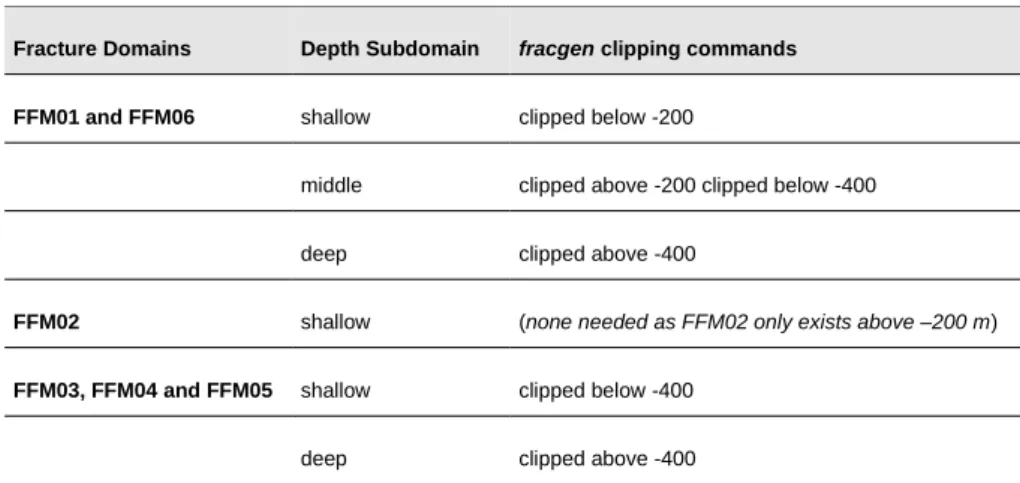
which contains all of the fracture domains defined by SKB. Input files for each specific domains were produced by hand-editing copies of this file to delete all other domains. Finally, subdomains for different depths as specified in Table C-1 of SKB R-08-95 (Follin, 2008) were defined by running the script create_depth_domains which inserts the appropriate fracgen clipping commands, as detailed in Table 2.1.

Fracture Domains Depth Subdomain fracgen clipping commands

FFM01 and FFM06 shallow clipped below -200

middle clipped above -200 clipped below -400 deep clipped above -400

FFM02 shallow (none needed as FFM02 only exists above –200 m)

FFM03, FFM04 and FFM05 shallow clipped below -400

deep clipped above -400

Table 2.1 Definition of fracture subdomains by depth. Note that the depth ranges for subdomains in FFM06

are the same as for FFM01, and the depth ranges for subdomains in FFM04 and FFM05 are the same as for FFM03.

2.1.2.

Fracture set definitions

The fracture population for the Forsmark model is simulated based on the statistical hydro-DFN model as specified in SKB R 08-98 Table C-1 (Follin, 2008). The fracture set statistics listed in that table were transcribed directly into fracture set definitions files for fracgen input, as listed in Table 2.2.

Fracture Domains Depth Subdomain Fracture set definitions file

FFM01 and FFM06 shallow FFM01shallow.sets

middle FFM01middle.sets deep FFM01deep.sets

FFM02 shallow FFM02shallow.sets

FFM03, FFM04 and FFM05 shallow FFM03shallow.sets

deep FFM03deep.sets

Table 2.2 List of fracture set definitions files used as input to fracgen, for generating fractures in the different

2.2.

Estimation of effective continuum properties

Three methods are applied to evaluate rock-mass hydraulic conductivity tensors K, porosities θ, and flow wetted surface ar for the DFN models used in SR-Site:

• Analytical and semi-analytical formulae for the contribution of each fracture set to the aggregate hydraulic properties, based on an assumption of fractures of infinite extent in an infinite domain;

• Block-scale DFN geometrical calculations based on summing the contributions of individual fractures for 20 m to 100 m block scales; • Block-scale DFN flow (permeameter) simulations.

The first two methods do not account for fracture connectivity effects, but provide quick approximations that can be used for scoping sensitivities. The semi-analytical methods apply to infinite domains rather than finite blocks, and thus do not account for scale effects or heterogeneity. The last method is more computationally intensive but is necessary to assess the validity of a K tensor in a sparsely connected DFN. Formulae and procedures for each of these methods are discussed in the following paragraphs.

2.2.1.

Analytical estimates of rock hydraulic properties

A simple analytical estimate of the flow wetted surface, ar is obtained directly from the conductive fracture intensity as:

a

_r

=

2P

_32c

summed over the fracture sets for a given fracture domain.

An analytical or semi-analytical estimate of the flow porosity θ can be obtained by integrating over the fracture transport aperture distribution to find the arithmetic mean aperture, and multiplying this by the areal intensity of conductive fractures per unit rock volume:

θ

_r

=

P

_32c

̄

_b

_T

For simple cases where aperture is independent of other fracture properties, the mean aperture can be found analytically as the first moment of the probability density function for aperture:

̄

b

_T

=

P

_32c

∫

0 ∞

b

_T

f

_b

₍

b

_T

₎

db

_T

In SKB's SR-Site models, the transport aperture bT is considered to be related to fracture transmissivity T by an empirical relationship bT = bT(T), specifically:

b

_T

[

mm

]

=

0 .5

(

T

[

m

2

/

s

])

0. 5

Fracture transmissivities are simulated based on a variety of correlation relationships with the fracture size (radius) r as the primary variable. For the cases in which there is a direct functional relationship between T and r, this gives the possibility of a fully analytical solution based on:

̄

b

_T

=

P

_32c

_∫

0 ∞

b

_T

(

T

(

r

)

₎

f

_r

(

r

)

dr

More generally (for example the case where T and r are semicorrelated), the mean aperture can be estimated numerically by stochastic sampling of the fracture size distribution:

〈 ̄

b

_T

〉

_N

=

1

N

∑

_i=0

N

b

_T

₍

T

₍

r

_i

₎

₎

where ri is the ith random sample from the size distribution fr(r). However, this type of estimate exaggerates the effect of the small-radius, small-aperture fractures and thus leads to an underestimate of porosity. A more appropriate average aperture is weighted with respect to fracture area

〈 ̄

b

_T

〉

_A

=

∑

i=0 N

A

₍

r

_i

₎

b

_T

₍

T

₍

r

_i

₎

₎

∑

i=0 N

A

₍

r

_i

₎

where for circular fractures A(ri) = π.. This area-weighted estimate is used in the present study.

An analytical estimate of the hydraulic tensor K due to a set of fractures with orientations the Fisher distribution fractures is obtained starting from the expression of Snow (1969) for the hydraulic conductivity tensor due to a set of parallel, infinite, uniformly spaced fractures, which may be written in matrix notation as:

K =

T

s

[

I −n n

⊗

]

where:

T = fracture transmissivity s = effective fracture spacing

I = the identity matrix with components Iii = 1; Iij = 0 for i ≠ j; i,j = 1,2,3,.

n = unit normal vector to fracture plane (i.e., the fracture pole)

and where

n n

⊗

denotes the outer (tensor) product with components ni nj, for i, j = 1, 2, 3.

For a set of fractures of infinite extent with poles (normal vectors) distributed according to a Fisher distribution:

f (θ, ;κ

ϕ ) = c( κ) e

κ cosθ where:

θ = angle from the mean pole direction of the fracture set.

ф = angle in the longitudinal sense about the mean pole,

and:

1

c (κ )

=

∫

₀ 2π

∫

0 π

e

κ cosθ

_{sin θdθd}

_{ϕ =}

4πsinh (κ )

κ

and assuming that fracture transmissivity is independent of orientation, the effective hydraulic conductivity tensor is found by integrating the differential contribution of each fracture orientation over the unit sphere:

K =

T

̄

P

_32c

c

(

κ

)

∫

₀ 2π

∫

0 π

where

T

̄

is the arithmetic mean transmissivity of the fracture set, and P32c is used in place of s as a directionally unbiased measure of spacing.

If we choose a working right-handed coordinate system (x1', x2', x3') such that x3' is parallel to the mean pole of the Fisher distribution θ = 0 and x1' coincides with ф =

0, then the matrix inside the integral may be written term-by-term as:

[

I−n n

⊗

]

=

[

1−sin

2

_{θ cos}

2

_ϕ

_sin

2

_{θ sin}

_{ϕ cos ϕ sin θ cosθ cos ϕ}

sin

2

θ sin

ϕ cos ϕ

1−sin

2

θ sin

2

ϕ

sin θ cos θ sin

ϕ

sin θ cos θ cos

ϕ

sin

2

θ sin

ϕ cos ϕ

1−cos

2

θ

]

Substituting this into the matrix integrand of the preceding equation and integrating  term­by­term yields the hydraulic conductivity tensor K' in the Fisher­aligned  coordinate system (x1', x2', x3'):

K' =

T

̄

P

_32c

[

1−πc (κ ) B (κ )

0

0

0

1−πc (κ ) B (κ )

0

0

0

2 πc (κ) B (κ)

]

where:

B

(

κ

)

=

∫

0 π

sin

3

θe

κcosθ

dθ =

4

κ

2

[

cosh κ−

sinh κ

κ

]

c (κ ) =

κ

4πsinh (κ )

This can be simplified and written more compactly as:

K' =

[

K

_t

0

0

0

K

_t

0

0

0

K

_p

]

where:

K

_t

=

T

̄

P

_32c

[

1−

coth κ

κ

+

1

κ

2

]

K

_p

=

2 ̄

T

P

_32c

[

coth κ

κ

−

1

κ

2

]

are the components of hydraulic conductivity transverse and parallel, respectively, to  the mean pole of the Fisher distribution.

Figure 2.1.Spherical polar coordinate system.

For the general situation, the components of the hydraulic conductivity tensor may  be required for a reference coordinate system (x1, x2, x3) or (x, y, z) which is not necessarily aligned with the mean pole of the Fisher distribution. Assuming that the mean pole is specified in spherical polar coordinates (Figure 2.1)as (θm,фm) where θm is the angle from the x3 direction (typically vertical) to the mean pole direction, and

фm)is the angle from the x1 direction to the projection of the mean pole into the x1 –

x2 plane, then by defining the rotation matrix A as:

A =

[

cos θ

_m

cos

ϕ

_m

−sin

ϕ

_m

sin θ

_m

cos

ϕ

_m

cos θ

_m

sin

ϕ

_m

cos

ϕ

_m

sin θ

_m

sin

ϕ

_m

−sin θ

_m

0

cos θ

_m

]

the hydraulic conductivity tensor in the reference coordinate system may be obtained as :

K = AK 'A

T

where the superscript T denotes the matrix transpose.

To obtain an analytical estimate of the hydraulic conductivity tensor for a fracture domain that contains multiple fracture sets, each with its own Fisher distribution parameters (mean pole direction and concentration), mean transmissivity, and P32c, the overall K tensor is calculated as the sum of the K tensors to each set.

Analogous to the calculation of a mean aperture, an area-weighted estimate of the mean transmissivity for use in the above analytical formulae can be obtained from simulations as:

〈 ̄

T 〉

_A

=

∑

i=0 N

A

₍

r

_i

₎

T

₍

r

_i

₎

∑

i= 0 N

A

₍

r

_i

₎

2.2.2.

Geometrical estimates of rock hydraulic properties

Block-scale estimates of the rock mass hydraulic properties K, θ, and ar can also be produced using geometrical calculations based stochastic simulations of the DFN model. In contrast to the foregoing analytical/semi-analytical methods, this approach accounts for the effects of finite fracture size and finite block scales, and produces estimates of spatial variability. However, as for the analytical methods, the geometrical methods described here do not account for connectivity effects. The basic approach in producing geometrical estimates of rock-mass hydraulic properties is to add up the contributions of individual fractures for 20 m to 100 m block scales. For these calculations, realizations of the complete site-scale DFN model are used, and properties are calculated for blocks at different positions in the reference coordinate system.

The contribution of a single fracture i to the block-scale tensor K is calculated from Snow's law (Snow, 1969) which, as in the preceding section, can be written in matrix form as:

K

_i

=

T

i

s

_i

[

I−n n

⊗

]

where: Ti = fracture transmissivity si = effective fracture spacing I = the identity matrix with components Iii = 1; Iij = 0 for i ≠ j; i,j = 1,2,3,. n = unit normal vector to fracture plane

and where

n n

⊗

denotes the outer (tensor) product with components ni nj, for i, j =  1, 2, 3. The effective fracture spacing si is taken as V/Ai where Ai is the area of the fracture  that lies within the volume V of the rock block (the entire area of the fracture, if the  fracture is entirely within the rock block).  The block­scale hydraulic conductivity tensor is then approximated as the sum of the  contributions of each fracture that has some portion within the block volume V:

K =

∑

i∈V

K

_i This method of estimation was originally proposed by Oda (1985). A drawback of this approximation is that it generally overestimates the block­scale  hydraulic conductivity that would be obtained by an explicit block­scale DFN  calculation. Not all fractures within a given volume will form part of the conductive  "backbone" of the through­flowing network, and network tortuosity further reduces  the effective hydraulic conductivity. However this approximation can be calculated  with much less computational effort than is required for the more rigorous approach  of permeameter simulations (as described below). Block­scale porosity is calculated as a scalar property:

θ =

∑

i∈V

b

_i

s

_i

=

1

V

∑

_i∈V

b

i

A

i

where bi is the effective transport aperture of the ith fracture. Note that this does not  take into account possible directional dependence of block­scale porosity, nor  network effects. A geometrical estimate of flow­wetted surface is calculated as a scalar property:

a

_r

=

2

V

∑

_i∈V

A

i Note that this similarly does not take into account possible directional dependence of  flow­wetted surface, nor network effects.

Depending on the goals of the simulation, geometrical estimates were produced either for all 6000 of the grid cells in the 6 km3 _volume:

X = 1 630 000 m to 1 633 000 m Y = 6 699 000 m to 6 701 500 m Z = -800 m to 0 m

with a cell size of (100 m)3_{, or for a random selection of 40 to 100 blocks from the}

same grid.

The latter approach was used in simulations where the fracture coordinates and properties were saved for permeameter simulations, so that geometric estimates could be compared directly with permeameter estimates. Due to the very large number of fractures in the full simulation volume, storing the fracture data for a full simulation was not practical.

The random selection of cells is done independently and randomly by an acceptance -rejection procedure to produce an unbiased sample of sites in 3-D. Figure 2.2 shows an example of the lateral and vertical distribution of cells that were sampled in one case.

Figure 2.2.Example of spatial distribution of sampled cells for combined geometric and permeameter estimation of rock mass hydraulic properties. Plot shows distribution of cell locations in plan view; table shows distribution in the vertical direction. The high proportion of cells at Z = -250 m in this example is an example of stochastic clustering; other realizations of the sampling scheme produced fewer cells in this depth range.

2.2.3.

Permeameter estimates of rock hydraulic properties

Block-scale permeameter simulations, by explicit modeling of flow through a DFN network model, can provide estimates of the effective directional components of K, as well as the estimates of the effective θ and ar for a given flow direction. This approach accounts both for the finite size of fractures and connectivity effects on the block scale. It also provides a possibility to evaluate the applicability of the

hydraulic conductivity tensor for a given block scale.

Methodologies for permeameter simulations to evaluate hydraulic conductivity tensors were investigated by Long et al. (1982) and subsequent authors. In the present study, a relatively simple methodology is used with simulations in just three orthogonal directions. This approach is intended as an initial analysis suitable for the current phase of review.

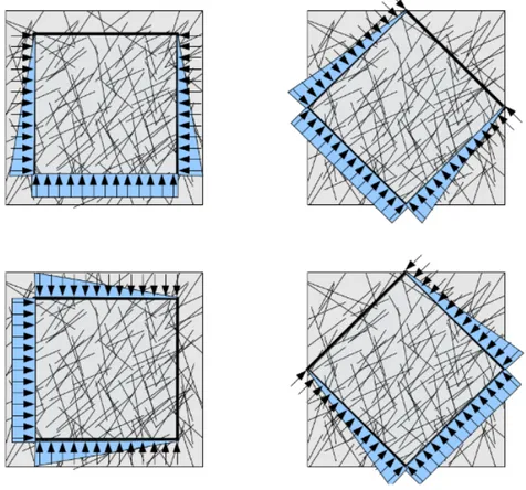
The procedure uses the same DFN simulations as for the geometric estimates, allowing direct comparison between methods. The fractures for a randomly selected subset of the blocks (as in Figure 2.2) are discretized within a cubical boundary to produce a finite-element mesh on the selected scale (20 m, 50 m, or 100 m), using the mesh-generation methods and algorithms of the DFM software (Geier, 2010).Flow simulations are then performed in each of the three orthogonal directions corresponding to the cubical boundary edges. A fixed head gradient is applied between the upstream and downstream ends of the cube, with linearly declining heads along the other boundaries (Figure 2.3). Effective directional hydraulic conductivities are calculated as the ratio of the flows to the applied head gradient, per unit cross-sectional area.

Figure 2.3. Schematic illustration of permeameter simulations with declining-head

boundary conditions.

A more detailed analysis could consider additional directions for the applied gradient, to test for consistency of the directional conductivities with the assumption of a hydraulic conductivity tensor. Another possible refinement could be use of “guard zones” along the sides with declining-head boundary conditions, to reduce the effect of flows through fractures that happen to cut across a corner. These refinements were not used in the present study but could be considered in further investigations if warranted.

Flux-weighted estimates of θ, and ar are produced from each directional flow simulation by integration over the calculated network flow fields. The estimates are weighted with respect to groundwater flux, so that the results represent primarily the pathways through each block (for the given direction of hydraulic gradient) that carry the bulk of the flow (generally less than the total fracture porosity and wetted surface, as obtained from the geometrical calculation methods described above).

Flux­weighted porosity for a head gradient parallel to the ith coordinate axis is  calculated as a weighted sum over all finite elements in the block­scale mesh, either  as:

〈

θ

_i

〉

_q

=

1

V

∑

e∈V

q

_e

b

_e

A

_e

∑

e ∈V

q

_e

〈

θ

_i

〉

_qA

=

1

V

∑

e∈V

q

_e

b

_e

A

_e2

∑

e ∈V

q

_e

A

_e where be is the effective transport aperture of the eth triangular finite element in the  mesh, qe is the magnitude of flux in that element, and Ae is its area. The first of these  estimates emphasizes the elements that carry the highest fluxes, regardless of their  size, while the second measure includes element area to reduce the tendency to skew  results toward a few small elements that might have very high local fluxes. Conceptually analogous flux­weighted estimates of flow­wetted surface are  calculated as:

〈

a

_r i

〉

q

=

2

V

∑

e∈V

q

_e

A

_e

∑

e ∈V

q

_e

〈

a

_r i

〉

qA

=

2

V

∑

e ∈V

q

_e

A

_e2

∑

e∈V

q

_e

A

_e

2.3.

Interaction of natural fractures with EDZ

This issue is investigated by embedding a section of deposition tunnel within realizations of a block-scale DFN model, and simulating flow due to hydraulic gradients imposed parallel and perpendicular to the tunnel axis.

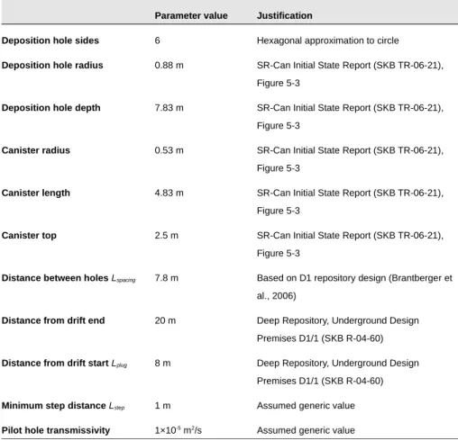
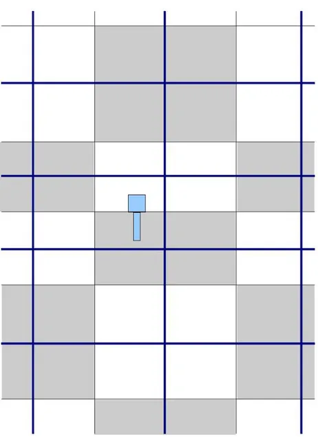
The tunnel is assumed to be backfilled, with either a continuous or discontinuous EDZ. Deposition holes are included to allow evaluation of fluxes to deposition holes, and advective-dispersive transport calculations as described below. The deposition holes positions are conditioned on the DFN realization to avoid fractures with full-perimeter intersections. The deposition holes are represented as vertical hexagonal prisms (Figure 2.4), following the methods of Geier (2011). Conditional placement of deposition holes for a given realization of the DFN is according to the FPC criterion of Munier (2010), as implemented in the DFM module repository (Geier, 2008). Parameters governing deposition hole geometry and placement along the tunnels are as listed in Table 2.3.

Locations of the blocks for these simulations are chosen randomly from the site-scale DFN model domain, but restricted to blocks that are centered at -450 m (as an approximation of the repository depth, to the nearest 100 m grid division).

While the location of the deposition holes can vary depending on the locations of large stochastic fractures, typically twelve deposition holes are simulated per 100 m block, after allowing space at both ends of the tunnel segment.

Four cases are considered for each block and tunnel segment:

• Continuous EDZ (all EDZ elements are retained with fixed transmissivity

TEDZ = 10-8 _m2_/s);

• 75% EDZ (25% of the EDZ elements are randomly assigned a very low transmissivity 10-5_{xTEDZ, so that flow will be focused in the remaining}

75%);

• 50% EDZ (50% of the EDZ elements are randomly assigned a very low transmissivity 10-5_xT

EDZ, so that flow will be focused in the remaining

50%);

• No EDZ (all of the EDZ elements are assigned a very low transmissivity 10-5_xTEDZ).

For each of these cases, flow fields are calculated by imposing an arbitrary but representative hydraulic gradient of 0.001 (on the order of the regional topographic gradient which is estimated as 0.00125; see Geier, 2012, Table 6.1), to drive flow in each of three orthogonal directions aligned with the cubical boundary: SW to NE (horizontal and parallel to the tunnel), SW to NE (horizontal and perpendicular to the tunnel), and vertically upward.

In each case and for each flow direction, an effective block-scale hydraulic conductivity is calculated as the mean flowrate divided by the cross-sectional area and the magnitude of the hydraulic gradient. Thus directional hydraulic

perpendicular to the tunnel, and vertical), for each of the cases of EDZ fractional continuity.

Table 2.3 Deposition hole parameters for the model.

Parameter value Justification

Deposition hole sides 6 Hexagonal approximation to circle

Deposition hole radius 0.88 m SR-Can Initial State Report (SKB TR-06-21),

Figure 5-3

Deposition hole depth 7.83 m SR-Can Initial State Report (SKB TR-06-21),

Figure 5-3

Canister radius 0.53 m SR-Can Initial State Report (SKB TR-06-21),

Figure 5-3

Canister length 4.83 m SR-Can Initial State Report (SKB TR-06-21),

Figure 5-3

Canister top 2.5 m SR-Can Initial State Report (SKB TR-06-21),

Figure 5-3

Distance between holes Lspacing 7.8 m Based on D1 repository design (Brantberger et

al., 2006)

Distance from drift end 20 m Deep Repository, Underground Design

Premises D1/1 (SKB R-04-60)

Distance from drift start Lplug 8 m Deep Repository, Underground Design

Premises D1/1 (SKB R-04-60)

Minimum step distance Lstep 1 m Assumed generic value

Pilot hole transmissivity 1×10-5 _m2_{/s Assumed generic value}

The flowrate to each deposition hole is calculated as the net flux crossing the deposition hole boundary. This corresponds to an open-hole condition rather than the case in which the hole is sealed with buffer. All deposition holes are intersected by the EDZ feature in the tunnel floor, and some are also intersected by stochastic fractures. Note that even in the “no EDZ” case, an EDZ feature of very low transmissivity intersects each deposition hole, though the groundwater flux may be negligible.

Flows to canister positions are calculated as the sum of all positive flows into the deposition hole (generally balanced by outflows).

The water velocity in the fractures intersecting the deposition holes is of interest for bentonite erosion modeling as well as for radionuclide transport. The mean velocity at the ith deposition hole was calculated as:

̄v

_i

=

∑

j∈i

Q

_j

∑

j∈i

L

_j

b

_Tj where:

Qj = flowrate across the jth element edge [L3_/T],

bTj = transport aperture at jth edge.

and where the sums are taken over all element edges j that intersect the ith deposition hole.

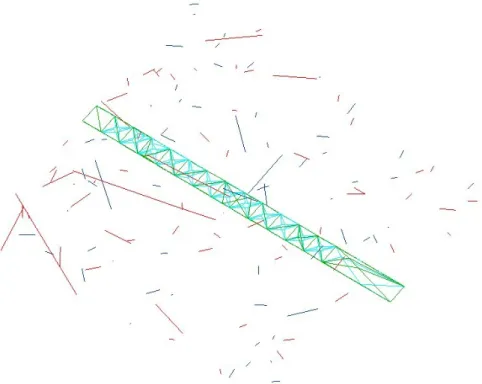
Figure 2.4.Plan view of finite-element mesh for the EDZ and deposition holes along a 100 m

long tunnel segment, oriented from SE to NW, for the investigation of EDZ interactions with natural fractures along deposition tunnels. Green line segments indicate the boundaries of triangular finite elements along the roof of the tunnel. Blue/aqua line segments are element boundaries for the EDZ in the floor of the tunnel, with the deposition holes appearing as small hexagons in this view. Dark red and dark blue lines represent intersections of the DFN fractures with the upper and lower faces (at -400 m and -500 m, respectively) of the 100 m cube that is used as the boundary for flow simulations to evaluate EDZ properties. Note that these are just a small fraction of the discrete fractures that are contained entirely or partly within the cube. However, the sparseness of these intersections on the upper and lower faces is indicative of the sparseness of the DFN model at repository depths.

Advective-dispersive particle tracking is used to characterize transport properties of paths from deposition holes through the rock mass and/or EDZ. This yields

estimates of water residence times tw, path lengths L, and transport resistance F for paths via the EDZ and/or the stochastic DFN on scales up to 100 m. The scale of 100 m is a representative value for transport via the EDZ and rock mass before reaching a hydraulically conductive, site-scale deformation zone; for example, in Figure 3-10 of Selroos and Follin (2009) it may be seen that nearly all deposition holes locations are within 400 m of the nearest deterministic deformation zones, most are within 200 m, and many are so close that the computational grid cell containing the deposition hole is also intersected by a deformation zone. Advective-dispersive transport of non-sorbing solute through the 3-D network (neglecting matrix diffusion) is modelled by the discrete-parcel random walk method (Ahlstrom et al., 1977). This approach represents local, 2-D advective-dispersive transport within each fracture plane. 3-D network dispersion, due to the interconnectivity among discrete features, arises as the result of local dispersion in combination with mixing across fracture intersections.

For mathematical details and definition of parameters see Geier (2005; 2008b). The algorithm assumes complete mixing at fracture intersections; this is a reasonable approximation for the low advective flow velocities expected in a post-closure repository, as discussed by Geier (2008a).

Particles are initiated from source locations, which in the present study comprise the intersections of transmissive features with the perimeters of the deposition holes. For each canister position that is intersected by a transmissive feature, 100 particles are released. Transport parameters used in this step are summarized in Table 2.4.

Table 2.4 Parameters for advective-dispersive particle tracking.

Parameter Feature Category Feature Set(s) Value

Molecular diffusion

coefficient All All 2.0x10

-9 _m2_/s

Ratio of transverse dispersivity to longitudinal dispersivity

All All 0.1

Longitudinal dispersivity Repository tunnels 1 1 m

2.4.

Sensitivity of fracture hydraulic properties to

future stress conditions

The sensitivity of rock-mass hydraulic properties to future stress conditions is investigated by calculating block-scale geometrical estimates of rock mass hydraulic conductivity and porosity (K and θ) due to predicted changes in effective rock stresses during future glaciations.

The method makes use of the relation between fracture normal stress and

mechanical aperture as defined in SR-Site (TR-11-01 p 333, Figure 10-20, based on Hökmark Figure 4-9):

e = e

_r

+

e

_max

e

−ασn

It is assumed that the fracture transmissivities simulated in each realisation of the DFN model are representative of the present-day stress conditions at their respective depths. By calculating the normal stress σn as resolved on the given fracture plane at the given depth, based on the SR-Site model for vertical and principal horizontal stresses as functions of depth, and the corresponding normal stress σn' _{for a given} future state of stress, the ratio of the future and present mechanical aperture is obtained from:

e'

e

=

e

_r

+

e

_max

e

−ασn'

e

_r

+

e

_max

e

−ασn

It is further assumed that transmissivity scales as the cube of mechanical aperture. On this basis the fracture transmissivity under the future state of stress is:

T' = T

(

e'

e

)

3

which can be used as the basis for block-scale geometrical calculations as described in Section 2.2.2. based on summing the contributions of individual fractures, after applying fracture normal stress vs. transmissivity models as described in the SR-Site data report.

Note that this approach does not account for connectivity or coupled stress-flow effects. It is intended only to provide a means for scoping changes in bulk hydraulic properties of the bedrock due to glacial loading.

The basic method for making these calculations was developed and implemented in the course of this modelling project. However, results are not presented due to lack of well-defined stress functions for future glacial loading states, and prioritization of other parts of the modeling project.

2.5.

Site-scale model development

A multi-scale discrete-feature model for the Forsmark site was developed based on modifications of a previous implementation by Geier (2010; 2011).Key

modifications to the previous model included the following:

 Shallow bedrock aquifer features trimmed to portions SSW of ZFMWNW0001 and NNW of ZFMENE0062A

 Equivalent features (K-lattice): Added vertical cell boundary at -468 m (deposition tunnel floor level) and shifted -420 m and -520 m levels to -448 m and -488 m so K values reflect only deleted fractures within 20 m of tunnels (as shown schematically in Figure 2.5);

 Repository: Includes vertical shafts (“generic” location due to restrictions on coordinates) and inclined access ramp with multiple sections for different sealing methods per TR 11-01 Figure 5-25.

 EDZ transmissivity in deposition tunnels is 10-8 _m2_{/s per TR-11-01, p. 295.}

 EFPC criterion for the Hydro-DFN now applies to any intersections with deposition hole (per TR-11-01, p. 152);

 Maximum transmissivity of deposition holes 10-10 _m2_{/s (integrated along}

length of deposition hole and averaged around wall, TR-11-01, p. 150); this constraint is applied post-simulation by identifying deposition holes that exceed this value.

Due to time constraints and prioritization of other aspects of this modeling project, only a few trial flow simulations of the revised site-scale model were attempted. These did not converge to adequately accurate solutions of the flow equations to provide reliable results for this project. Therefore a detailed explanation of the refined model is omitted from this technical note.

Figure 2.5.Schematic illustration of design of grid cells and equivalent-continuum features to avoid artefacts of these features intersecting deposition holes. Shaded gray and white areas represent grid blocks; blue lines indicate schematic locations of equivalent features to represent the effective hydraulic conductivity of the grid blocks.

3. Results and Analysis

3.1.

Estimation of effective continuum properties

Equivalent continuum properties K, θ, and ar for the rock mass were obtained by

three methods, as detailed in Section 2.2: • Analytical/semi-analytical estimates;

• Block-scale DFN geometrical calculations based on summing the contributions of individual fractures;

• Block-scale DFN flow (permeameter) simulations to calculate effective directional components of K, and flux-weighted estimates of θ, and ar.; The results of these calculations are presented in the following subsections.

3.1.1.

Analytical estimates of rock hydraulic properties

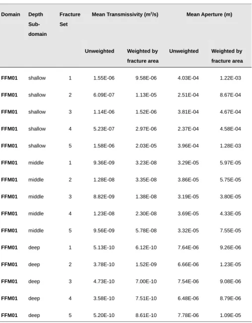
The analytical expressions for rock mass hydraulic properties, as given in Section 2.2.1, require suitable average values of fracture transmissivity and transport aperture, for each fracture set and domain. Due to the complicated density functions for these variables, and correlations with fracture radius (and thus fracture area) which are implicit in the semi-correlated model for fracture transmissivity, stochastic simulation was used to obtain appropriate estimates.

The results for Fracture Domain FFM01 are listed in Table 3.1. Equivalent results were obtained for the other fracture domains, but are omitted here for the sake of space, and because FFM01 is the domain of primary interest for flow within the proposed repository.

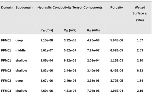
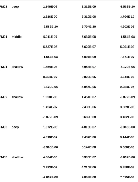
Using these values, the analytical formulae in Section 2.2.1 were applied to obtain estimates of the hydraulic conductivity tensors, porosity, and flow wetted surface for each fracture domain and depth subdomain. These results are summarized in Table 3.2. The full K tensors including off-diagonal components are listed in Table 3.3.

Domain Depth Sub-domain

Fracture Set

Mean Transmissivity (m2_{/s) Mean Aperture (m)}

Unweighted Weighted by fracture area

Unweighted Weighted by fracture area

FFM01 shallow 1 1.55E-06 9.58E-06 4.03E-04 1.22E-03

FFM01 shallow 2 6.09E-07 1.13E-05 2.51E-04 8.67E-04

FFM01 shallow 3 1.14E-06 1.52E-06 3.81E-04 4.67E-04

FFM01 shallow 4 5.23E-07 2.97E-06 2.37E-04 4.58E-04

FFM01 shallow 5 1.58E-06 2.03E-05 3.96E-04 1.28E-03

FFM01 middle 1 9.36E-09 3.23E-08 3.29E-05 5.97E-05

FFM01 middle 2 1.28E-08 3.35E-08 3.86E-05 5.75E-05

FFM01 middle 3 8.82E-09 1.38E-08 3.19E-05 3.80E-05

FFM01 middle 4 1.23E-08 2.30E-08 3.69E-05 4.33E-05

FFM01 middle 5 9.56E-09 5.78E-08 3.32E-05 7.55E-05

FFM01 deep 1 5.13E-10 6.12E-10 7.64E-06 9.26E-06

FFM01 deep 2 3.78E-10 1.52E-09 6.66E-06 1.23E-05

FFM01 deep 3 4.73E-10 7.00E-10 7.54E-06 9.08E-06

FFM01 deep 4 3.58E-10 7.51E-10 6.48E-06 8.79E-06

FFM01 deep 5 5.20E-10 8.61E-10 7.78E-06 1.09E-05

Table 3.1 Mean transmissivities and mean apertures calculated from multiple simulations (total of 4,752,520

fractures), for fracture domain FFM01. Equivalent estimates were obtained for the other fracture domains but are omitted for the sake of space.

Domain Subdomain Hydraulic Conductivity Tensor Components Porosity Wetted Surface ar

(1/m)

K11 (m/s) K22 (m/s) K33 (m/s)

FFM01 deep 2.15e-08 3.32e-08 4.20e-08 5.64E-06 1.07

FFM01 middle 5.01e-07 5.62e-07 7.27e-07 6.07E-05 2.03

FFM01 shallow 1.85e-04 9.82e-05 2.08e-04 1.16E-03 2.30

FFM02 shallow 1.83e-06 2.44e-06 3.40e-06 6.49E-04 6.33

FFM03 deep 1.67e-06 2.49e-06 3.36e-06 3.79E-05 1.54

FFM03 shallow 4.60e-06 4.21e-06 7.08e-06 1.93E-04 2.19

Domain Subdomain Hydraulic Conductivity Tensor Components Kij (m/s)

FFM01 deep 2.146E-08 2.316E-09 -2.553E-10

2.316E-09 3.319E-08 3.794E-10

-2.553E-10 3.794E-10 4.203E-08

FFM01 middle 5.011E-07 5.637E-08 -1.554E-08

5.637E-08 5.622E-07 5.091E-09

-1.554E-08 5.091E-09 7.271E-07

FFM01 shallow 1.854E-04 8.954E-07 -3.120E-06

8.954E-07 9.823E-05 4.044E-06

-3.120E-06 4.044E-06 2.084E-04

FFM02 shallow 1.828E-06 1.454E-07 -6.872E-09

1.454E-07 2.436E-06 3.689E-08

-6.872E-09 3.689E-08 3.402E-06

FFM03 deep 1.672E-06 4.818E-07 -2.366E-08

4.818E-07 2.487E-06 3.144E-08

-2.366E-08 3.144E-08 3.360E-06

FFM03 shallow 4.604E-06 3.393E-07 -2.657E-08

3.393E-07 4.210E-06 9.858E-08

-2.657E-08 9.858E-08 7.075E-06

3.1.2.

Geometrical estimates of rock hydraulic properties

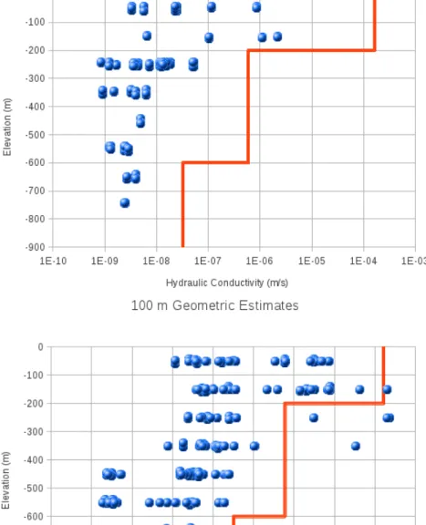
Geometrical estimates of scale rock hydraulic properties are shown in Figures 3.1 through 3.3, for hydraulic conductivity, porosity, and flow-wetted surface respectively. The analytical estimates for the different depth intervals of fracture domain FFM01 are shown as red lines for comparison.

The geometrical estimates of block-scale hydraulic conductivity are mostly lower than the analytical estimates, particularly for the smaller 50 m block scale (Figure 3.1). Similarly, the geometrical estimates of porosity and flow-wetted surface (Figures 3.2 and 3.3) tend to be lower than the analytical estimates. However, heterogeneous distribution of fractures arising from the stochastic simulation gives rise to many blocks with lower estimated values, and a few blocks with higher estimated values of these properties.

A possible explanation for the closer agreement between the geometrical and analytical estimates on the 100 m block scale may be that the larger blocks tend to be dominated by a few large fractures. These large fractures tend to be significantly more transmissive, because of the semi-correlated relationship between fracture size and fracture transmissivity T. This affects the hydraulic conductivity distribution most strongly due to the linear relationship between T and K, but also carries into the porosity estimates due to the assumed proportionality of transport aperture to the square root of T.

Geometrical estimates of flow-wetted surface show a weak correlation to hydraulic conductivity (Figure 3.4). A correlation in these estimates is expected because blocks with more fractures (and hence more fracture surface area per unit volume) tend to have higher hydraulic conductivity. The weakness of the correlation may be due to the strong effect of large, high-transmissivity fractures which contribute to the

K tensors in proportion to the product of T times area, but contribute to the wetted

surface estimates only in proportion to their area.

A bimodality is apparent in the results for hydraulic conductivity (Figure 3.1), particularly at depths below Z = -300 m. Comparison with a larger set of geometric estimates from a single realization (Figure 3.5) shows that this bimodality persists and becomes more clear in the larger simulated data set.

Cross-sections of geometrical estimates for the full set of grid cells (Figures 3.6 through 3.8) show that the bimodality arises from different parts of the simulated domain, corresponding to the different fracture domains. Distinctly lower K values (visible as the dark green area in the cross-sections from Z = -450 m and deeper) are found within fracture domain FFM01 (i.e. inside the “tectonic lens”) at depth, compared with the outer fracture domains.

At shallower depths this bimodal pattern is reversed, with higher K values in the inner part of the domain (visible as yellow to orange cells), and lower K values outside this.

Figure 3.1.Geometrical estimates of hydraulic conductivity versus depth for (a) 50 m and (b)

100 m block scales, plotted as the mean (Kx+Ky+Kz)/3. The red line in each plot shows the

corresponding analytical estimate of hydraulic conductivity for FFM01, depending on depth. Results shown are for a single realization in which fracture data were saved for randomly selected grid cells, for comparison with permeameter simulations.

Figure 3.2.Geometrical estimates of porosity versus depth for (a) 50 m and (b) 100 m block scales. The red line in each plot shows the corresponding analytical estimate of hydraulic conductivity for FFM01, depending on depth. Results are for the same realization and sampling of grid cells as in Figure 3.1.

Figure 3.3.Geometrical estimates of flow-wetted surface versus depth for (a) 50 m and (b) 100 m block scales. The red line in each plot shows the corresponding analytical estimate of hydraulic conductivity for FFM01, depending on depth. Results are for the same realization and sampling of grid cells as in Figure 3.1.

Figure 3.4.Geometrical estimates of flow-wetted surface versus hydraulic conductivity for the 100 m block scale. Results are for the same realization and sampling of grid cells as in Figure 3.1.

Thus the DFN model for Forsmark is found to produce contrastingly high conductivity in the shallow part of the “tectonic lens.” This effect is in addition to the the “shallow bedrock aquifer” which is included explicitly in the Site Descriptive Model for hydrogeology. The estimated hydraulic conductivity tensors throughout the model are dominantly horizontal (Figure 3.9).

Together with the generally elevated K values at shallow depths, the horizontal anisotropy of the DFN model can be expected to produce predictions of site-scale groundwater flow in which flow is focused through the upper part of the “tectonic lens.” Thus the geometrical properties of the DFN lead to a result that is is consistent with this key aspect of SKB's site interpretation.

Figure 3.5.Geometrical estimates of hydraulic conductivity versus depth (negative elevation Z)

for 100 m block scales, plotted as the mean (Kx+Ky+Kz)/3. The red line in each plot shows the

corresponding analytical estimate of hydraulic conductivity for FFM01, depending on depth. Results shown are for a single realization in which geometrical estimates of hydraulic conductivity were calculated for all grid cells. A random perturbation δZ, with |δZ| ≤ 25 m, has been added to the Z coordinate as a visualization aid to show where results are more strongly clustered; the actual grid cell centers are all at exactly Z = 50 m – n(100 m) where n = 1, 2, …, 8.

Figure 3.6Cross-sections showing geometrical estimates of DFN hydraulic conductivity at depths ranging from -50 m to -750 (right column), for a single realization of the DFN model

(FMSRblocksnp01). The color scale ranges from 10-14 _{m/s (dark blue/black) to 10}-1 _{m/s (dark}

red). Blank (white) areas are outside of the defined fracture domains. The rectangular area shown is bounded by the coordinate ranges (x,y) = (1 630 000 m, 6 699 000 m) to (1 633 000 m, 6 701 500 m).

Figure 3.7 Cross-sections showing geometrical estimates of DFN hydraulic conductivity at

depths ranging from -50 m to -750 (right column), for a single realization of the DFN model

(FMSRblocksnp02). The color scale ranges from 10-14 _{m/s (dark blue/black) to 10}-1 _{m/s (dark}

red). Blank (white) areas are outside of the defined fracture domains. The rectangular area shown is bounded by the coordinate ranges (x,y) = (1 630 000 m, 6 699 000 m) to (1 633 000 m, 6 701 500 m).

Figure 3.8Cross-sections showing geometrical estimates of DFN hydraulic conductivity at depths ranging from -50 m to -750 (right column), for a single realization of the DFN model

(FMSRblocksnp03). The color scale ranges from 10-14 _{m/s (dark blue/black) to 10}-1 _{m/s (dark}

red). Blank (white) areas are outside of the defined fracture domains. The rectangular area shown is bounded by the coordinate ranges (x,y) = (1 630 000 m, 6 699 000 m) to (1 633 000 m, 6 701 500 m).