THERMAL INTERNAL BOUNDARY LAYER
HEIGHT BY NUMERICAL SIMULATION OF
THE FUMIGATION
M.R. Sahebnasagh
1V. Esfahanian
2KH. Ashrafi
3M.khakshour
4 1Ph.D., National petrochemical company, NPC, Tehran, Iran
2 Departments of Mechanical Engineering, University of Tehran, Tehran, Iran
3
Department of Environmental Engineering, University of Tehran, Tehran, Iran
4
M.S., Environment researcher
ABSTRACT
Fumigation is an important subject in air pollution. In a neutral atmosphere, temperature decreases with the height. However, when there is a transient condition of climate like sunrise in the morning which leads to increase the land surface temperature, temperature profile of stable condition will change. In these conditions, convection of air near the ground surface increases the turbulence and dispersion coefficient. In coastal area, there will be a temperature difference between the sea and land. This condition make the pollutants to fumigate when enters to the layer above the ground named as Thermal Internal Boundary Layer (TIBL). The height of TIBL which defines the extent of fumigation is important. Researchers suggested several formulas for estimating the TIBL height based on practical works. In this paper, computational fluid dynamic (CFD) provides discrete phase model (DPM) of dispersion using Reynolds stress transport model of turbulence (RSM) applied for estimating the TIBL height. Study domain is two dimensional, 2500 m in wind direction (sea to land) by 800 m height. Velocity profiles of the neutral atmosphere are forced to the model in neutral steady state atmospheric conditions. Resulted profiles in downwind of the inlet are compared with the forced profiles to evaluate the accuracy of the model. To simulate the fumigation, land temperature fixed to a higher temperature than the sea by 5°c. Resulted velocity profile and gradient of Reynolds stress parameters u ' u ' and u ' v' in different elevations is used to
estimate the TIBL height. The location of sharp change in the Reynolds stress specified as the TIBL height at each elevation. A formula covering the coordination of these locations fitted to define the TIBL height and its growing from coastline towards wind direction. Experimental formula which is used can be substituted by the determined formula this study.
KEYWORDS
1 INTRODUCTION
Fumigation is a phenomena which occurs in coastal areas. It is of the air pollution scientists concerns particularly in vicinity of industrial complexes nearby the urban areas. When a new industrial plant is planned, new emissions are proposed or production change is expected. This has particular relevance for the authorization to operate the industrial plant where ambient considerations need to be assessed for human health and ecological reasons. Wind velocity and temperature profiles have a significant effect on the dispersion of the pollutants from the stacks or vents of the industries.
Fumigation and trapping are the results of inversion. On a flat terrain, stack plumes released in an unstable or convective boundary layer are subjected to vertical diffusion until they occupy the earth's surface and the capping inversion layer. In trapped plums the vertical concentration still decreases with distance due to horizontal diffusion or spreading. Trapping can lead to very high ground-level concentrations when the inversion height is low because of strong subsidence, weak winds, or slow heating of the surface [1]. The level of the inversion base is often used as an approximation for the mixing height although the former can be substantially (5-25%) smaller than the later [2].
Computer models for calculating dispersion of pollutants within the atmosphere have been available for many years and are generally applicable over scales up to about 50 km from release point [3]. Commercial CFD software, such as Fluent (www.fluent.com), offers a method for modeling flow and dispersion. Fluent offers the flexibility to represent the complex conditions such as plume dispersion under various temperature and velocity profile, ground heat flux and wind flow turbulence. CFD simulation can provide detailed output of flow fields (e.g. dead zones and accelerated flows), turbulence levels and concentration fields downwind of pollutant source. Kouchi et al.[4], investigated the effect of Thermal Internal Boundary Layer (TIBL) on Ground Level Concentration (GLC) and turbulent statistical properties in a thermally stratified wind tunnel. Numerical simulations using a Lagrangian stochastic dispersion model were also conducted and its results were compared with wind tunnel results and field observation. They assumed Gaussian distribution for u and v
components of velocity within the TIBL region. It was a comparison between a developed model and an experimental study. Luhar and Sawford [5] tested several fumigation models. They observed that many existing models that assume uniform and/or instantaneous vertical mixing in the TIBL, give inaccurate results for large entrainment rate and/or small vertical plume spread at the plume-TIBL interface. They developed an improved analytical fumigation model based on a probability density function (PDF) approach.
Advanced numerical methods are new approaches in environmental studies that can be used for realistic simulation of pollutants dispersion in inversion conditions. In this study the fumigation is simulated to find out the TIBL height at downstream of a wind direction coming from see to land in coastal areas using control volume method by CFD Fluent software. In order to enforce the temperature, velocity, turbulence and dissipation rate profiles the user-defined function facility of the software is implemented.
The paper is organized as follows: Firstly, the governing equations that are used in Fluent are presented. The boundary conditions of numerical simulation are discussed and then temperature and velocity profiles are defined. The plume dispersion set up is outlined and the numerical simulation results are presented. Finally the conclusions of the study are presented.
2 GOVERNING EQUATIONS
Governing equations of motion of the atmospheric air which is a completely turbulent flow including the continuity, momentum and energy shown here are discretized and numerically integrated in Fluent. Continuity: m i i S u x t ∂ = ∂ + ∂ ∂ ) (ρ ρ (1) Momentum: i i j ij i j i j i g F x t x p u u x u t ∂ + + ∂ + ∂ ∂ − = ∂ ∂ + ∂ ∂ ρ ρ ρ ) ( ) ( (2) Where, ⎥ ⎥ ⎥ ⎥ ⎦ ⎤ ⎢ ⎢ ⎢ ⎢ ⎣ ⎡ − − − − − − − − − = ) ' ( )' ' ( )' ' ( )' ' ( ) ' ( )' ' ( )' ' ( )' ' ( ) ' ( 2 2 2 w v w w u w v v u v w u v u u t zz zy zx yz yy yx xz xy xx ij τ τ τ τ τ τ τ τ τ Energy: h j i ij i i j j j i i eff i i S x u x p u t p J h x x T k xi h u x h t ∂ + ∂ + ∂ ∂ + ∂ ∂ + ∑ ∂ ∂ − ⎥ ⎦ ⎤ ⎢ ⎣ ⎡ ∂ ∂ ∂ ∂ = ∂ ∂ + ∂ ∂ ′ ′ ′ τ ρ ρ ) ( ) ( ) ( (3)
where ρ is density, t is time, x is the i i th direction, u is velocity component in i x direction i
and S is source term of the mass, p is static pressure, m tij is shear tension tensor, ρgi and
i
F are gravity force and other outer force in i th direction, respectively, h is static enthalpy,
dT
c
h
T T j P j ref∫
=
' ' ,Where, c is specific heat at constant pressure, p J j′ is diffusion flux of j′th component,
)
( t
eff k k
k = + is effective conductivity, and k is turbulent thermal conductivity. t S is heat h
source.
Discrete phase model of fluent is used for pollutant dispersion. In this model, the pollutant molecules are considered as particles which injected from source point. The following equation of motion is applied on particles:
x p p x p D p F g u u F dt du + − + − = ρ ρ ρ ) ( ) (
Where, u is fluid phase velocity,
p
u is the particle velocity, FD (u − up) is drag force, ρpis
the density of the particle and Fx are the other forces on it.
The Fluent software solves the 2D Reynolds averaged equations for air flow, pressure, turbulence parameters and energy field [6]. The Reynolds stress terms are provided by Reynolds stress transport model (RSM) which is found to be more suitable for air pollutant dispersion [7]. There are five equations in 2D and seven in 3D for the Reynolds stress in RSM turbulence modeling as:
(
) (
)
(
)
(
)
(
)
(
)
Term Source Defined User user Rotation System by oduction F ikm m i ikm m j k n Dissipatio k j k i Strain essure i j j i oduction Boyancy G i i j i oduction Stress P k i k j k j k i Diffusion Molecular D j i k k Diffusion Turbulent D j ik i kj k j i k convection C j i k k derivative local j i S u u u u x u x u x u x u p u g u g x x u u x u u u u u x x u u p u u u x u u u x u u t ij ij ij ij ij ij T ij T ij . . . . . . Pr ' ' ' ' ' ' . Pr ' ' Pr . ' ' Pr . ' ' ' ' . ' ' . ' ' ' ' ' ' ' . ' ' 2 2 , , + + Ω − ∂ ∂ ∂ ∂ − ⎟ ⎟ ⎠ ⎞ ⎜ ⎜ ⎝ ⎛ ∂ ∂ + ∂ ∂ + + − ⎟⎟ ⎠ ⎞ ⎜⎜ ⎝ ⎛ ∂ ∂ + ∂ ∂ − ⎥ ⎥ ⎥ ⎦ ⎤ ⎢ ⎢ ⎢ ⎣ ⎡ ⎟⎟ ⎠ ⎞ ⎜⎜ ⎝ ⎛ ∂ ∂ ∂ ∂ + + + ∂ ∂ − = ∂ ∂ + ∂ ∂ = = = = = = = = ε ε ρ μ θ θ ρβ ρ μ δ δ ρ ρ ρ ε φ (4) The terms ij TD , , Gij , φij and εij is modeled to close the equations as described in Fluent user
guide [6]. SIMPLE method is used to discretize the governing equations (i.e., pressure, velocity, temperature, concentration). Other theoretical aspects and boundary conditions are discussed in next sections.
3 SET UP OF THE BOUNDARY CONDITIONS
A 2D domain with a length of L= 5000 m and a height of h=800 m is considered for performing the numerical simulation. Wind speed of 5 ms-1 (at reference height of 10 m above the ground) and a ground roughness length of 0.1 m, represented agricultural land, are used to calculate the profiles of velocity, TKE and turbulent dissipation rate in domain of study. Velocity profile calculated based on the following experimental relation [2].
) ln( ) ( 0 0 * z z z u z u = + κ for z ≤ h (5)
where, u(z) is the wind speed at a height of z above the ground, z0 is the roughness length, u*
is the friction velocity which is calculated using reference height velocity, h is the domain height and κ is Von Karman's constant (0.4). The temperature profiles are defined based on the stability conditions of the atmosphere which are discussed later in this section. The TKE and dissipation rate profiles are considered similar to the profiles used by sahebnasagh et al [9]. Upstream boundary conditions of these profiles are set at inlet to the domain of study. Atmospheric air as inlet fluid to the domain considered as incompressible perfect gas with variable density. Study domain surface is discretized with an unstructured mesh, with greater resolution of the nodes close to the ground. Ground (z=0) is specified as a stationary wall with a specified roughness (z0=0.1). The lines of x=-2500 m and x=2500 m are specified as inlet
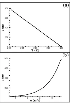
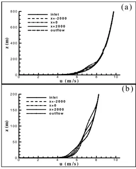
and outflow boundaries, respectively. Also z=800 m is specified as symmetry plan. Characteristics of the generated unstructured grid are shown in Figure 2. Figure 3 shows the inlet profiles of neutral temperature and velocity. Neutrally stable temperature profile considered as adiabatic laps rate, equal to -0.01 ْ Km-1. The inlet TKE and dissipation rate profiles are shown in Figure 4. To check the accuracy of the model, the inlet forced velocity profile of neutrally stable atmospheric conditions are compared with the downwind locations profiles resulted from simulation. The predicted profiles of velocity resulted from running the model show no significant change in downstream as shown in figures 5(a) and 5(b). These figures compare the velocity profiles throughout the domain for two cases, up to the height of 800 m and 200 m, respectively. As shown in Figure 5(b) main change in velocity profile occurs only near the ground due to wind shear as it is expected [10]. The predicted TKE profiles generated by turbulence model at different downward locations of the inlet boundary are shown in Figure 6.
As illustrated in this figure, the TKE level reduces to about 30% of the inlet value at the ground which is similar to the results founded by Sahebnasagh et al. [10]. The inlet TKE
Figure 2: Generated grid of domain
profile development throughout the downstream is consistent with the atmospheric boundary layer theory. Turbulent effect begins from the end of sublayer. Outside the sublayer up to 10 m, that is called roughness layer, viscous and turbulent effects coexist. Surface layer including sublayer and roughness layer extends to the height of the order of 100 m (turbulent core) from the ground. In the region named as outer layer, above surface layer, turbulence effect reduces to its minimum at free atmosphere [2], [8].
The TKE level increases from zero to its peak value well within the surface layer. Figures 5 and 6 indicate good agreement of the result of the model with the results obtained by Sahebnasagh et al [9],[10],[11]. This ensures the accuracy of the model to be applied for predicting the pollutant dispersion patterns in the atmosphere.
u (m/s) z( m ) 6 7 8 9 200 400 600 800 (b) T (K) z( m ) 292 294 296 298 300 0 200 400 600 800 (a)
Figure 3: Inlet profiles (a) temperature and (b) velocity
T ue bule nt dissipa tion ra te (m 2 /s3 )
Z( m ) 1 0-4 1 0-3 1 0-2 1 0-1 0 2 0 0 4 0 0 6 0 0 8 0 0 (b) TK E (m 2 /s 2 ) z( m ) 0 .2 0 .4 0 .6 0 .8 1 2 0 0 4 0 0 6 0 0 (a)
u ( m / s ) z( m ) 0 2 4 6 8 1 0 0 2 0 0 4 0 0 6 0 0 8 0 0 in le t x = - 2 0 0 0 x = 0 x = 2 0 0 0 o u tflo w (a ) u ( m / s ) z( m ) 0 2 4 6 8 1 0 0 5 0 1 0 0 1 5 0 2 0 0 in le t x = - 2 0 0 0 x = 0 x = 2 0 0 0 o u tflo w (b )
Figure 5: Velocity profiles comparison throughout the domain (a)up to 800m.(b) up to 200m + + ++ + +++ + + + ++ ++ + ++ + + ++++ +++++++++++++ ++++++++++ ++++++++ ++++++ ++++++ + + + + + + + + + + + + + + + + + + + + + + + + + + + + + + + + + + + + + + + + + + + + + T K E ( m 2 /s 2 ) Z( m ) 0 .2 0 .4 0 .6 0 .8 1 1 .2 0 2 0 0 4 0 0 6 0 0 8 0 0 in le t x= - 2 0 0 0 x= 0 x= 2 0 0 0 o u tflo w +
Figure 6: TKE profiles development from inlet to downwind
T ( K ) z( m ) 2 9 4 2 9 6 2 9 8 3 0 0 0 2 0 0 4 0 0 6 0 0 8 0 0 in le t x = - 2 0 0 0 x = 0 x = 2 0 0 0 o u tflo w
Figure 7 shows a similar result for the temperature profiles throughout the domain. As shown
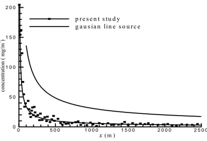
in this figure, the simulated profiles are approximately the same as the inlet to the domain. Since the lateral dispersion is ignored in 2D studies, it is reasonable to compare the results with the line source dispersion models. Figure 8 shows the concentration at source height with Gaussian line source model for neutral case. For this comparison average of 10 snap shots is used to eliminate the turbulence fluctuation effects.
( m ) con ce nt rati on ( m g/m 3 ) 0 5 0 0 1 0 0 0 1 5 0 0 2 0 0 0 2 5 0 0 0 5 0 1 0 0 1 5 0 2 0 0 p re s e n t s tu d y g a u s ia n lin e s o u r c e x
Figure 8: Concentration of plume at source height, comparison of present study with Gaussian line source formula
The trends of the both curves are similar and difference is due to dispersion model used. Limitations of the gaussian model lead to overestimate the concentration of pollutant at near field [2].
4 TEMPERATURE PROFILES
Among the main parameters that specify the atmospheric inversion conditions are temperature and velocity profiles. Effect of the other parameters such as humidity on dispersion patterns is ignored in this study. To investigate the fumigation phenomena and clearly determining the TIBL, temperature profile of stable atmospheric conditions is considered at inlet to the domain of study, see Figure 9. Moreover, the wind velocity profile generated from equation (5) is considered at inlet to the domain in upstream.
5 PLUME DISPERTION SET UP
The Lagrangian particle (LP) tracking model within Fluent has been used for simulating the pollutant dispersion. Particles are released from stack and their movement tracked based on
atmosphere (considered enough large time to ensure the steady state condition) is simulated by Fluent CFD code. Source data are as follows:
• Source location: x=-1500 m, z=100 m • Source height: 100 m
• Emission particle diameter: 1e-5 m
• Emission velocity: vx=0.0 ms-1, vz= 20 ms-1 • Emission flow rate: 0.01 kgs-1
• Temperature: 450 ْ K
Characteristics of generated grid (Figure 2) and Fluent set up of the model are: • Unstructured grid of 21376 cells
• Reynolds stress model of turbulence
• Discrete phase model (DPM) of pollutant dispersion
Using RSM model when particle tracking is implemented and turbulence fluctuations for individual directions of coordination are used, leads to a non isotropic simulation. It should be noted that the resolution of the particle method is limited by the number of particles tracked. Thus the method cannot simulate the very low concentrations (i.e., the concentrations below 0.0010 μgm−3 in this case).
Figure 9: Temperature profiles corresponding to stable conditions under fumigation
Grid study is made by checking the +
y (a non-dimensional wall distance) for the first cell. A
+
y value of about 30 is most desirable [6]. To fulfill this limitation, y + value is adopted
using adoption option in Fluent and excessive stretching in the direction normal to the wall is avoided.
6 RESULTS AND DISCUSSION
Specific conditions of the ambient temperature and wind velocity profiles which lead to fumigation are forced as inlet boundary conditions of temperature and wind velocity to the model. Result of dispersion of pollutant under this condition is shown in Figure 10. This figure show that present model takes into account turbulence theories and boundary
conditions that are specified for, otherwise considerable errors of implausible concentrations would have been produced at the boundaries.
Since under fumigation conditions, TIBL starts to grow from coastline towards downstream of wind flow, so it is expected that some parameters related to the turbulence and pollutant dispersion to be change drastically at TIBL boundary. To estimate the TIBL height and its growing rate on land, the rate of change of turbulence kinetic energy, Reynolds stress of
2 '
u and w '2 is studied at levels of 40 to 160 meter above the land at increments of 20 m. to
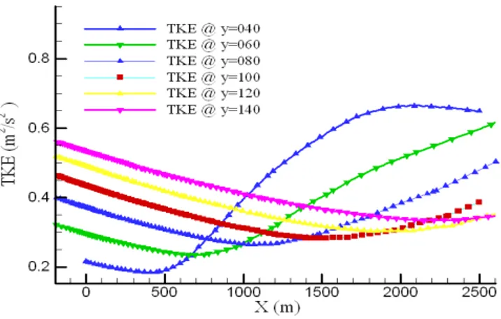
check the hypothesis, the result compared for two cases, with and without temperature difference of the land and sea surface. The result showed that the drastic change of the mentioned parameters does not exist when there is no temperature difference between the land and sea surfaces. The point of drastic change of these parameters are the TIBL boundary cross point with the wind flow at that level. Considering the physics of the fumigation, expecting the drastic change of these parameters can be used to calculate the equation of TIBL height. Since it is the result of solving the exact governing equation of motion and energy, determined equation for TIBL height is expected to be more accurate than the previous analytical and experimental one. Temperature difference between land and sea (ΔT), and convection heat transfer coefficient near the land are 20 ْc and 20 w/m2.k respectively. Figure 11 shows the TKE curves of each level from upstream toward downstream. The
Positions of drastic change of this parameter at each level are in Table 1. Pendgrass and Arya (1984), Viemmy et al.(1995), Gart(1995) has introduced an equation of h=axn which, h is TIBL height and x is the distance from coast line. “a” and “n” are constant coefficients. They have introduced the constant coefficients based on their analytical and experimental estimation. Considering the similar equation but using the exact data from Table 1, the new equation is introduced for TIBL height by 0.333 and 0.77 for “a” and “n” respectively. Figure
12 show the TIBL height calculated from new equation and compared with the result of the
equation introduced by Pendegras and Arya. The rate of growing the TIBL height is similar for two equations but due to exact solution of the governing equations the new introduced equation is more accurate to use in environment studies.
Figure 11. TKE curves at various levels of atmosphere under fumigation
Table 1: coordination of the drastic change of the TKE
Figure 12: TIBL height calculated from new formula and compared with Pendegrass and Arya
7 CONCLUSION
Atmospheric temperature and velocity profiles dictate the atmospheric conditions of environment studies. The new equation for TIBL height which is very important for fumigation phenomena and dispersion of pollutant near coastlines is shown in this study.
The LP model is based on the stochastic tracking of particles using the individual turbulent fluctuations from the RSM model, thus giving the non-isotropic formulation. The set up of the model for plume dispersion requires consideration of the grid selection of appropriate turbulence and dispersion models. The recommended setup conditions determined from this study are listed below:
Atmospheric air to be considered as a incompressible ideal gas Reynolds stress turbulence model
Velocity, temperature, turbulence model and dissipation profiles specified at the inlet +
y Adaptation is required for better results. It should be more than 30 as suggested by
Fluent CFD code.
It is important to specify correct or realistic boundary conditions for TKE and ε at the inlet.
Using excessive stretching in the direction normal to the wall should be avoided. Grid study to be checked by adopting the y value of the cells adjacent to the wall. +
The new introduced equation for TIBL is more accurate than the equations introduced before by the others because it is the result of solving the solution of exact governing equations of fumigation conditions. The other parameters of the dispersion and the atmosphere like temperature and Reynolds stress are studied for the subject matter too. Reynolds stress is same as TKE but its change is not as drastically as the TKE. Temperature due to graduate change in atmosphere is not reliable parameter for the subject matter. Captioned formula in this study can be used for environment study of air pollution under fumigation conditions. Since the temperature difference of the land and the sea is changed, so the equation can be revised for various ΔT.
Of the most important result, one may consider these parameters in conjunction with dominant temperature, velocity and TIBL height while designing the flares, chimneys, vents and stacks or allocate the new industrial plants near coastlines. It is well understood that the fumigation phenomena happens due to temperature difference between the land and sea and sea breeze condition. Knowing the TIBL height can be used for estimation of the mixing length and pollutant dispersion height.
8 ACKNOWLEDGEMENT
The authors would like to thank the university of Tehran and National Petrochemical Company (NPC) for providing research facilities.
9 REFERENCES
[1] Wark, K., Warner, C.F., Davis, WT., 1998, Air Pollution its Origin and control, third edition, Addison- Wesley Longman, Inc., U.S
[2] ARYA, S.P. (1999). Air Pollution Meteorology and Dispersion. (Oxford University
Press Inc.)
[4] Kouchi, A., Ohba, R., and Shao, Y. (1999). Gas Diffusion in a Convection Layer Near a Coastal Region. Wind Engineering and Industrial Aerodynamics, NO.81, 171.
[5] Luhar, A.K., and Sawford, B.L. (1996). An Examination of Existing Shoreline Fumigation Models and Formulation of an Improved Model. Atmos. Environ. V.30, NO.4, PP. 609-617. [6] Fluent 6.2.16 user’s guide,( 2002), Fluent Inc. Available from www.fluent.com.
[7] Muralidhar, K., and Biswas, G. (2005). Advanced Engineering Fluid Mechanics. second edition, (Alpha Science International Ltd. Harrow, U.K.)
[8] Sahebnasagh, M.R., Esfahanian, V., Gitipour, S., Ahmadi, G., Ashrafi, Kh., 2008, Simulation of Plume Patterns Associated with Different Atmospheric Temperature Profiles,
Asian Journal of chemistry, Vol 20, No. 8, pp 6551-6564
[9]Sahebnasagh, M.R., Esfahanian, V., Gitipour, S, Nabi bidhendi, Gh., Ashrafi, Kh., Numerical Simulation of plume Patterns under Various inversion Layer Heights,
International Journal of Environment Research, under publicati
[10] Sahebnasagh, M.R., Esfahanian , V., . Ashrafi, KH., 2009, Numerical simulation of plume patterns under various inversion layer heights, 17th international conference of Air