Pay-as-you-speed: An economic field-experiment
Lars Hultkrantz*
ab,Gunnar Lindberg
b* Corresponding author: Örebro University, 701 82 Örebro, Sweden, +46-19 30 14 16, lars.hultkrantz@oru.se,
a
Swedish Business School, Örebro University, bSwedish National Road and Transport Research Institute
Acknowledgements: We are grateful for suggestions on previous versions of this paper
by Sara Arvidsson and Jan-Eric Nilsson, and participants at the Transportation Research Conference, Strassbourg, The 2nd Nordic Conference on Behavioural Economics,
Göteborg, The International Transport Economics Conference, Minneapolis, and seminar participants at The Swedish Institute of Industrial Economics, The Swedish National Institute of Road and Transport Research, Örebro University, and Växjö University.
Abstract
We report a vehicle-fleet experiment with an economic incentive for keeping within speed limits using a speed-alert device. A traffic insurance scheme was simulated with a monthly bonus during two months reduced by a non-linear speeding penalty. Participants were randomly assigned into four treatment and two control groups. A third control group consists of drivers who had the device and were monitored, but did not participate. We find that participating drivers reduced severe speeding during the first month, but in the second, after having received feedback reports with an account of earned payments, only those given a penalty changed behaviour.
1.0 Introduction
Traffic insurance contracts provide no direct incentives to car drivers that comply with maximum speed limits, although speeding is a major accident risk factor that increases the probability of occurrences and the severity of consequences. In this study, we
evaluate a simulated insurance scheme that gives such an incentive. Voluntary enrolment to a speed-compliance scheme is encouraged with a monthly participation reward (bonus) while speed-limit violations are disciplined by a small per-minute charge (penalty). The penalty is step-wise increasing in the relative magnitude of the difference between actual speed and the speed limit. This mechanism was tried in a economic field experiment for two months with 114 cars equipped with “Intelligent Speed Adaption (ISA)” in-vehicle GPS devices that warn drivers with flashing light and sound when driving faster than the stipulated maximum-speed limit.
Modern information and communication technologies, together with better digital maps, has brought a variety of “Intelligent Traffic Systems (ITS)” in-vehicle devices with a potential of enhancing the performance of traffic systems through navigation, steering, display of traffic signs, speed control etc. Many such services have a private goods nature and have been merchandized for years, either as supplementary equipment or as
integrated components of vehicles. However, other such services have a private bads nature, although they may provide public goods, and are therefore difficult to sell on a purely commercial basis. ISA services generally belong to the second category. Although they may be helpful to people with some self-control problem, who therefore want to be alerted when they drive too fast, in most cases speeding is a deliberate and conscious choice by the driver, so having for instance a flashing and noisy speeding alert is just an
annoyance. From a social point of view, however, the driver may be ignoring external effects of speed on safety and pollution, and after all, there normally are good motives for having speed limits. Our study investigates a method for reconciling the private and the social interest in using such equipment.
The present study is also related to the prevailing trend in insurance towards “Usage-Based-Insurance (USI)”. A prominent USI example is “Pay-As-You-Drive” traffic insurance programmes, where insurance premiums are paid by driven mile (Parry 2005). Such programmes are offered in several countries based on a similar technology as the one we use in this study. Our scheme is hence another example of USI that can be called “Pay-As-You-Speed (PAYS)”.
In insurance, USI schemes potentially offer solutions, or at least mitigation, to various moral hazard and adverse selection problems. Also, the theory of propitious selection (Hemenway 1990, de Meza and Webb 2001, Cohen 2005, de Donder and Hindriks 2005, 2009) suggests that there are risk-avoiding personalities who both take physical precautions and buy insurance. DeDonder and Hindriks (2009), in an analytical study of insurance market equilibrium, show that under some mild regularity assumptions, such preferences still do not imply a negative correlation between risk and insurance coverage at equilibrium. However in another analytical study within a mechanism-design framework, Arvidsson (2008) shows that a voluntary PAYS scheme can be designed so as to attract precautious drivers that already are more prone to compliance with speed rules. Complementary to this effect, such a scheme will sort out less precautious drivers, that is, those drivers who prefer to not join the programme. Thus PAYS can be used to create propitious, rather than adverse, selection in a separating equilibrium. The intuition
behind this result is that PAYS reveals otherwise private information on the degree of cautionary behaviour to the insurance company.
The focus of our study is, however, on moral hazard effects among users, not on selection effects. We study how some features of a PAYS scheme, the magnitude of the participation bonus and the penalty fee, affect driving behaviour of those drivers that have accepted to participate. The car drivers in our experiment had been initially
recruited to another study on a voluntary basis but without any remuneration. Thus, they can be assumed to be highly motivated for installing the ISA equipment, and probably for using it. However, since we could monitor driving behaviour of drivers that declined from participation in the economic experiment, we are able to provide some observations on self-selection of participants, and also to use non-participants as a control.
Finally, our study is related to the literature on internalization of external cost of transport. This issue has been at the top of the transport policy agenda for a long time. It has for long been acknowledged by policy-makers and economists that there is a need for more differentiated price or tax instruments. For instance, the petrol tax can be used as an instrument for imposing the external cost of carbon dioxide emission on the individual motorist, but does not differentiate between driving in densely or sparsely populated areas that may differ widely with respect to congestion, pollution exposure, etc.
Hitherto, measures have focused on (rough) internalization by driven distance (Parry 2005). The possibility to provide direct incentives to drivers for speed compliance was mentioned in this literature already by Boyer and Dionne (1983, 1987) but never explored because ‘it is usually either very difficult or extremely costly to observe
most societies instead rely on a combination of regulations (speed limits), enforcements (fines) and insurance schemes (deductions and bonus/malus). A common problem of all these instruments is the limited possibility to observe actual behaviour. However, the development of new technologies, as the Global Positioning System (GPS), mobile communications and improved information infrastructure (digital maps) now has changed this.
It should be noticed that incentives based on such improved possibilities of
monitoring individual drivers do not necessarily involve “Big Brother” integrity problems. This is so only if detailed vehicle position information is stored and conveyed, not just used for instantaneous measurement. What actually is needed to record for incentive purposes, is summary statistics at an aggregate level.1
Our main finding is that the speeding penalty substantially reduced the frequency of severe speeding violations. During the second experiment month, after having received feedback, participating drivers that were not given a speeding penalty did not
significantly reduce severe speeding.
In the next section we describe the design of the experiment. We then report results, first comparing participants and non-participants and then the different treatment groups to each other. Finally follows a discussion of these results.
1
For instance, a monthly or annual summary of the number of minutes the vehicle has been used for driving at a speed exceeding speed limits by a certain percentage.
2.0 The design of the field experiment
Our field experiment was designed for the purpose of evaluation of a PAYS insurance based on ISA equipment. A vehicle-fleet trial is very costly but we were given an
opportunity to use an already existing fleet trial. Vehicles for this trial had been recruited through an offer to a random sample of 1000 private car owners in a Swedish city
(Borlänge, pop. 48 000) to get ISA equipment installed free of charge. No other
economic incentives were used in this trial. 250 private car owners accepted to have their vehicles provided with on-board computers with digital maps, GPS positioning and mobile communication facilities. The technical system informed the driver about the speed limit on a display in the vehicle while an acoustic signal and a flashing light alerted him or her if the vehicle was driven faster than the speed limit (Bergeå and Åberg 2002).
The original trial was completed in December 2001. Early next year, the car owners were informed that they could keep the equipment for some time if they wanted. During the late spring, we invited 114 private car owners that still had these devices installed to participate in an economic experiment for two months (September and October 2002).These months were chosen for the main experiment, because they are free from the two major seasonal “distortions” in this part of Sweden:, that is, summer
vacations (from mid June to mid August) and winter road conditions (November – March), both having major effects on aggregate travel and speeding patterns. After the second experiment month was completed, however, we had not exhausted the project budget so we offered the participants to continue for a third month. As will be shown later, that turned out to be of no use since winter came during that month.
In our experiment, car owners were informed that they would receive a monthly bonus of 250 SEK or 500 SEK to be paid immediately at the end of the month. However some persons were informed that this bonus would be reduced by a penalty each minute they drove faster than the speed limit. The size of the penalty varied in four steps between 0 and 1 SEK per minute, or between 0 and 2 SEK per minute, depending on the
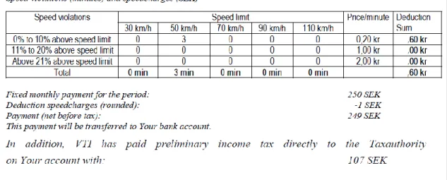
magnitude of speed violations2. All participating drivers, also those that would get the lump-sum bonus without penalty reductions, got individual feedback reports on their total time of driving and speeding, together with the monthly bonus payment.
Those owners that accepted to participate were randomly assigned to a high or low initial bonus (250 SEK/month or 500 SEK/month), and to the three penalty categories (zero penalty; 0 – 1 SEK/minute; and 0 – 2 SEK/minute; respectively). To always make participation beneficial in monetary terms, there was a cap to the total penalty charges so that even high offenders would get a net payment of at least 75 SEK each month. As it later turned out, no one was even near of hitting this ceiling.
A majority of the car owners (95 persons out of 114) accepted to participate in the experiment, while nine drivers rejected, and ten did not respond. Drivers that accepted were hence randomly divided into six groups as shown in Table 1. There were 16 drivers in each of the groups A-E and 15 drivers in group F.
A remaining group (G) consisted of the 19 drivers that rejected or did not respond to the offer to take part in the economic experiment. These non-participators were still using the equipment and had been informed that their driving would be continued to be monitored for research purposes. This give us opportunity both to cast some light on
2
At this time 1 USD≈ 1 EURO ≈ 9 SEK, so the highest charge corresponded to roughly 20 cents per minute.
selection effects and to have a control group, although not randomly selected, with zero bonus, zero penalty, and no individual feedback reports.
Table 1 here
The four-step penalty scheme is progressive to reflect that accident risk increases progressively with the speed of the car (Nilsson 2000). The levels of the low penalty charge were set so as to correspond to the estimated external cost of speed choice, according to a cost-benefit model used by the Swedish National Road Administration. Hence, since the technical speeding detection probability is one (or close to one), this penalty scheme approximates a pure pigovian fee on speeding.3
Those given the low penalty scheme were charged 0.10 SEK per minute when the actual speed exceeded the speed limit by 0-10 percent, 0.25 SEK per minute when speed was 11-20 percent above limit and 1.00 SEK per minute for speed offences above 20 percent. Those car owners that were given the high penalty scheme were charged twice as much.
The experimental design makes it possible to control for a variety of effects. First, the non-participating group G offers control over effects on speeding evoked by external factors, such as change of weather conditions. Second, the zero-penalty groups A and B control for Hawthorn effects from being participator in an experiment, in which every
3
A comparision to a coarse estimate of the expected cost of speed fines indicates that the penalty fees levied in our field experiment were much larger, by a 104 order of magnitude, than the expected cost of speed tickets. Speeding fines in Sweden at this time varied between SEK 600 – SEK 1500. The average probability of getting a speeding ticket during a car trip in Sweden is approximately 0.2*10-6 (annual number of speeding tickets divided by annual number of car trips). Studies indicate that 50 percent of cars on Swedish road are speeding (Forward 2006). Therefore conditional on that a car is speeding, the expected cost of speeding fines per car trip was SEK 0.24*10-3 - SEK 0.60*10-3 . Finally, we assume that an average car trip lasts 20 minutes.
participant is given feedback information on his/her own driving behaviour. Third, the two bonus levels control for income effects, or other possible effects from the size of the participation bonus.4 Finally, the two penalty levels make it possible to evaluate both the effect of penalties vs. no penalties (comparing C and E to A, and D and F to B) and to effect of the size of penalties (comparing C to E and D to F). However, it must be borne in mind that the experiment groups are small. Also, unfortunately, due to technical failures of some equipment the year before our experiment, we lack some reference driving data, in particular for October 2001.
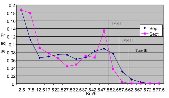
Data records were automatically collected once a month through mobile communication. The data contains information on geographical X- and Y-coordinates, time and date. This information was recorded frequently (every second or every tenth second) as long as the car engine was running. The data is summarized as individual speed profiles for each road type (defined as roads with different speed limits). As an example, Figure 1 presents the speed profile for one participant (car number 58) on roads with the speed limit 50 km/h in September 2001 and September 2002. This participant belongs to Group D. In this case, it seems that the driver has reduced severe speeding frequency, while instead increased the frequency of driving just below the speed limit.
As the technology was known from the technical trial to have some flaws, data was filtered from outliers to protect drivers from erroneous charging. At the end of each
4
In behavioural economics, a general observation is that many people behave in a reciprocal manner (Rabin 1993) including the phenomenon of “conditional cooperation” (Fehr and Fishbacher 2002), that is, that people contribute (to a common good) contingent upon others contribution. This could imply that drivers that were given the high participation reward would contribute more (high compliance to speed rules). Another possible effect of bonus size comes from “corner effects”, that is, that a driver with low bonus is more close to the penalty cap (SEK 75) where the marginal cost of further speeding is zero.
period, the participants received information about their speeding behaviour, the sum of penalty charges and the remaining net bonus (Figure 2).
Figure 1 here
Figure 2 here
In the individual feedback reports to the participants, speed violations were divided into three severity classes; Minor (0-10%), Medium (11-20%) and Major (≥ 21%). The reports stated the total time (minutes) during one month (t) that the car (i) had been driven faster than the speed limit, in total, Vit, and within each severity class,Vijt. By
dividing these variables with the total travel time of the car during the same month, Mit,
we compute the following speeding frequencies as our main outcome variables for evaluation of the economic interventions:
it ijt ijt V M S / , (1a) and i ijt it S S (1b)
The speeding frequency variables thus measure the proportion of total travel time that the car is used for driving faster than the speed limit, in total and within each severity class.
As it is likely that a reduction of Medium and Major speeding can result in a increase of Minor speeding, our evaluation will focus on the two most severe categories. In fact, in preliminary regression analysis, we found only small differences in models for these two categories, so regression results will be reported for the sum of them, which will be called Severe speeding.
An evaluation of a randomized experiment like ours can be based on
paired-difference tests, comparing across groups the paired-difference of the outcome variable during
one of the experiment months with the level of the same variable during a reference month, which here will be the same month one year before. Thus, for drivers for which we have all observations, we compare the levels of the outcome variables in September and October 2002, respectively, to these levels in September and October 2001,
respectively. However, since our sample is small, and is further reduced by lack of observations for some drivers in 2001, especially in October, randomization may not be fully effective as a means of controlling for differences between individuals. Our evaluation of results will therefore be based on regressions, using observations of all individuals, and controlling for individual covariates, that is, not on comparison of group by group averages.
3.0 Results
The results of the field experiment will now be reported in four consecutive steps. First, searching for self-selection effects, we compare descriptive statistics and previous driving behaviour of the group of drivers that accepted to participate in the economic experiment to the group of drivers that rejected participation (but remained being monitored). Also, we discuss tentatively how the participating drivers relate to the general population of motorists in Sweden. Second, we compare changes in average speeding time between participants (groups A-F) and non-participants (group G). Third, we compare changes in average speeding time each month across the six experiments groups (A-F) of drivers that took part in the economic experiment. Finally, we report regression results based on observations on the individual level where we control for some individual characteristics.
3.1 Characteristics of participants and non-participants
As shown in Table 2, the average participating car owner (Group A-F) was 57 years old and had an annual income of SEK 384 000. The participants were therefore on average older and had higher income than the car owners in general.5 26 percent were female (national average is 31 percent). Non-participants (Group G) were on average 5 year younger and had an even higher income than participants, but only the age difference to participants is statistically significant.
Table 2 also compares average Total and Severe speeding frequency of
participants and non-participants during September and October 2001, respectively, that is, one year before the economic experiment. According to the evaluation of the
technology trial in 2001, the average speed of drivers was reduced by 3 percent when the ISA equipment was activated (that is, during the autumn of 2001), compared to a
previous reference period when the equipment was silent (but was used to record driving behaviour).
The table shows that before the experiment, participants on average drove faster than the speed limit around 14 percent of the driving time, while non-participants were on average speeding 17 percent of the driving time. This difference is, however, not
significant. For Severe speeding, the proportion of driving time was 4 percent for participants and 6 percent for non-participants. This difference is significant at the five
5
The average age of a car owner in Sweden is approximately 46 years (SIKA 2006). The average annual income of full time employees in 2001 was SEK 295 000.
percent level. However, the significance disappears in a regression controlling for the individual covariates (Sex, Age, Age squared, and Income), see Appendix Table A1.
Table 2 here.
As already noticed, both these two samples have emerged by stepwise self-selection from the original random sample of car-owners in Borlänge that were offered a possibility to take part in the technical trial. Some indication on how these selections affect speeding behaviour can be inferred from a recent opinion poll on attitudes to speeding among 13 000 Swedish citizens6, showing that men, younger persons (age 25-39) and persons with higher income (increasing across several income levels) tend to have a more lax attitude towards speeding than women, older person (age 40-69) and persons with lower income. The high average age in our sample suggest that initial attitudes before the experiment (and presumably behaviour) leaned more towards compliance to speeding rules, compared to the national population of drivers7, but the low female share and high average income may give a tendency in the opposite direction.
6
The poll was commissioned by an insurance company (Länsförsäkringar 2008). Respondents were aksed in telephone interview: “How serious do you regard the following legal violation: speeding”. Response alternatives were “very serious”, “not so serious”, “nothing to care about” and “no opinion”. Unfortunately, only cross-tabulations of results were reported.
7
This conclusion is based on the finding in the poll that there is a substantial difference in attitude between individuals of age 25-39 and of age 40-69. In the younger group, 31 percent regarded speeding as a serious violation of legal rules (while 67 percent responded “not so serious” or “nothing to care about”). In the older group, 46 percent considered it serious (while 52 percent responded “not so serious” or “nothing to care about”).
3.2 Effects on participants and non-participants
In this section we report results for all treated groups as a whole (participants, that is, groups A-F)) and compare to non-participants (group G). Thus we compare two groups in which all individuals have active in-vehicle devices, but in which one (non-participants) did not get feed-back reports nor bonus, and another (participants) in which all
individuals got feed-back reports and a bonus, and some also had penalty reductions.
Table 3 here.
Table 3 shows, for September and October, the average 12-month differences in the proportion of total travel time that drivers were speeding. This is shown for
participants and non-participants, respectively.
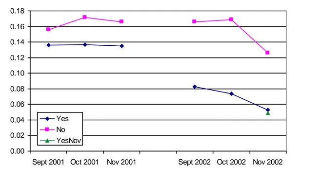
First, it can be observed from this table that the non-participants did not reduce the speeding frequency. This is as expected and gives some support to our approach to evaluate the results of the experiment from 12-months differences, that is, there is no indication that these differences are confounded from changes of external conditions. In contrast, as shown in Figure 3 below, showing the average total speeding frequency of participants and participants for all three autumn months of 2001 and 2002, non-participants on average considerably reduced speeding from October to November 2002, but not from October to November 2001. The explanation is that winter-road conditions arrived more early in 2002 than in 2001.
Second, returning to the September and October results shown in Table 3, we see that in comparison to the same month one year before, participants on average reduced speeding time by 5-6 percentage units of total travel time (corresponding to around 40 percent decrease of total speeding time both months). The differences between
participants and non-participants in these 12-month differences are significant for all violation types except for the highest speeding class in October.
3.3 Impacts across treatment groups
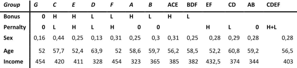
We now turn to differences of impacts across the randomly selected treatment groups among participants. An initial question to be asked in a randomized experiment is whether the randomization successfully balanced subject´s characteristics across the different treatment groups. To illuminate that question, Table A2 in Appendix shows the average values of the three key socio-economic variables sex (female = 1, male = 0), age (years) and total annual income (1000 SEK) for non-participants (G), the six randomized treatment groups (A-F), and various aggregates of the treatment groups.
The table indicates some undesired differences in these variables between the treatment groups, due to the small group sizes. These differences however, as expected, are reduced when groups are aggregated into larger entities. Anyhow, the upshot is that the limited sample sizes make it necessary to use regression to control for observable differences among individuals by regression.
To get a first tentative overview of the main results, however, Figures 4 and 5 make pair wise comparisons of different aggregates of treatment groups with respect to
one-year differences in speeding frequencies (Minor, Medium, Major and Total) for September and October, respectively.
Figure 4 compares non-participants (G) with the zero ((A+B), low (C+D), and high (E+F) penalty levels groups, respectively. We see that all participant groups on average considerably reduced speeding of all categories in September. In October, however, this effect remained for Severe speeding (Medium and Major) among groups with penalty charges, but not in the zero penalty group. For these violations, the relative difference between the entities without and with penalty charges is substantial (around 50 percentage units).
Figure 4 here.
Figur 5 compares non participants (G) with the low (B+D+F) and high (A+C+E) bonus groups. The figures indicate that, if anything, effects were larger in groups with the low bonus level, in particular in October.
Figure 5 here.
3.4 Regression results
As noticed in the previous section, due to small sample size randomization into experiment groups may be not fully effective in controlling for the effect of differences across individuals. We therefore now proceed by OLS regression focusing on the Severe speeding violations. To gain efficiency, we use a general to specific estimation procedure.
We start by regression of a “base” model in which the one-year differences of each of the speeding variables are regressed linearly on individual covariates and binary treatment variables indicating participation (yes/no), penalty (yes/no), high bonus yes/no) and high penalty rate (yes/no), respectively, where yes is represented by one and no by zero. Then, a selection of interaction variables are introduced one by one and kept if significant at lowest (10%) level, otherwise excluded (in fact, all were). Next, the model is step-wise reduced by elimination of the variable with the lowest t-value, until no t-value is below the critical value corresponding to the lowest level of significance. Then, finally,
interaction variables are introduced one by one as in the second stage. We report both the base model and the final parsimonious model.
Tables A3 and A4 in Appendix describe characteristics of the variables of the September and October samples we use. The sample sizes are mainly restricted by limited number of observations of driving (speeding) behaviour in 2001, which leaves 81 and 48 observations in the two samples, respectively. There also are a few observations of the income variable missing.
Table 5 shows the estimated general and specific models estimated for one-year differences of Severe speeding in the two samples. For the September difference, two variables, Age and Participation, remain in the reduced model; together explaining 12 percent of the total variation. In the reduced October difference model, the three
remaining variables are Penalty, Sex and Income*Sex; explaining 47 percent of the total variation.
The regression results support the conclusion that subjects of all treatment groups reduced Severe speeding during the first experiment month, while only subjects in groups
that were given speeding penalties reduced Severe speeding during the second month. No other treatment variables (or interactions, not shown) were significant.
Age enters the reduced September model with a negative coefficient but with a weak significance (p-value 0.096), while it gets a highly insignificant positive coefficient in the general October model. The summary tables in the Appendix do not indicate any unbalance in the age variable between the two samples. This effect is therefore difficult to interpret.
The reduced October model indicates that female subjects on average reduced their severe speeding, while male subjects with high income increased severe speeding. Both coefficients are significant. However, the general September model gives no support to this pattern, revealing highly insignificant coefficients for both Sex and Income. The summary tables do not indicate that these differences are connected to missing observations – income averages are quite similar and the differences in female shares suggest that most missing observations are among men, therefore not aggravating any possible problem of the data of a low number of female subjects.
4.0 Discussion and conclusions
We have conducted an economic field experiment with speed alert equipment during two consecutive months in a medium-sized Swedish city. 114 cars were monitored and of them 95 participated in the economic experiment. The participants were divided in six groups given either a high or a low participation bonus, and either zero, low or high penalty reduction of this bonus according to a progressive payment scheme reflecting the
social external cost of speed-limit violations. Between the first and the second month, participants were given a feed –back report on their speeding behaviour during the first month and an account of how much they would be paid.
Although the drivers were initially selected by a random sample of car-owners in the city, the sample of 114 drivers is not a representative sample of the general population. The sample is on average older, has higher income and includes more men than a
representative sample. It is not clear whether that implies that the sample drivers are likely to violate speeding rules more than the general population, but given that these subjects have voluntarily accepted to install speed alert devices, our best guess is that they are more inclined towards safe driving than the general population. We found that the motorists who accepted the offer to take part in the economic experiment were on average older that those who rejected or did not respond.
During the economic experiment participants significantly reduced their speed violations compared to non-participants. The time proportion of speed violations was reduced from around 15 percent of total driving time prior to the experiment to between 8 percent and 5 percent during the experiment with the lower interval at the end of the experiment period. Non-participants had almost constant proportion violations during the experiment.
During the first experiment month the priced participants reduced the speed violations more than the zero-penalty participants but the difference was not significant. However, during the second month priced participants reduced severe violations
significantly more than the zero-penalty group; the former had a reduction of 64 percent while the latter only had a reduction of 15 percent. Regression analysis gives statistical
evidence of a participant effect in September and a penalty effect in October. This implies that a penalty charge is essential for having a lasting effect on severe speeding, that is, the “placebo” or “Hawthorn” effects of participation that seem to be present in the September sample is not statistically significant in October.
Further, the results do not indicate any difference between the two penalty charge levels. This suggests that drivers have had a binary decision, either to change or not to change their regular behaviour, and that, at least for the duration of our experiment, the low level was high enough to exhaust the potential for that. This further suggests that a more simple scheme than the four-tier penalty rate we used would suffice, for instance a flat charge per minute for speed violations exceeding the speed limit by a certain margin.
Finally, there was no significant behavioural difference between groups with different bonus levels.
Our study thus suggests that economic incentive schemes, in the form of
insurance programmes or otherwise, coupled to the use of speed alter devices may be an effective way of reducing severe speeding, and thereby to increase overall road-traffic safety. The results imply that even drivers that voluntarily have installed such devices in their cars may be highly sensitive to economic incentives.
Needless to say, more research is warranted. Our study was performed at a time when speed-alert systems were a technical novelty. Now, such systems are becoming common either through supplementary navigation systems or as standard systems in premium cars. The quality of digital maps with update information on speed rules has improved greatly. It should therefore be possible to extend field experiments of the type
we have made to include larger, and perhaps more representative, groups of drivers, and to study effects during longer periods.
References
Arvidsson, S. (2008): „Reward Safe Driving: Applying Mechanism Design on Compulsory Vehicle Insurance‟, Working Paper, Örebro University, Dept of Economics.
Boyer, M. and G. Dionne (1983): „Sécurité routière : efficacité, subvention et réglementation‟, Université de Montréal, Publication #3030, Juin 1983.
Cohen A. (2005): ‟Asymmetric Information and Learning: Evidence from
The Automobile Insurance Market‟, The Review of Economics and Statistics, 87:197-207. de Donder, P. and J. Hindriks (2006): ‟Does Propitious Selection Explain
Why Riskier People Buy Less Insurance?‟ Working Paper no 2006017. Uni- versité catholique de Louvain, Département des Sciences Economiques.
de Donder, P. and J. Hindriks (2009): ‟Adverse selection, moral hazard, and propitious selection, Journal of Risk and Uncertainty 38(1):73-86.
De Meza, D. and D. Webb (2001): ‟Advantageous Selection in Insurance Markets‟, RAND Journal of Economics, Summer 2001: 249-262.
Hau, T.D. (1994): „A Conceptual Framework for Pricing Congestion and Road Damage‟, in B. Johansson and L.-G. Mattsson (ed.) Road Pricing: Theory, Empirical
Assessment and Policy, Kluwer Academic Publishers.
Hemenway, D. (1990): ‟Propitious Selection‟, Quarterly Journal of Economics 105:1063-1070.
Hurst, P.M. (1980) :„Can Anyone Reward Safe Driving?‟, Accident Analysis and
Prevention, Vol 12, 1980, pp 217 – 220.
Janson, J.O. and G. Lindberg (1997): „PETS - Pricing European Transport Systems - Pricing Principles‟, European Commission 1997.
Jansson, J.O. (1994): „Accident Externality Charges‟, Journal of Transport
Economics and Policy, 28(1), 31 - 43.
Johansson, O. (1996): Welfare, externalities, and taxation; theory and some road
transport applications. Gothenburg University, dissertation.
Jorgensen, F.J. and J. Polak (1993): „The effect of personal characteristics on driver‟s speed selection: an economic approach‟ Journal of Transport Economics and
Policy, 27(3), 237 – 252.
Lindberg, G. (2000): „Marginal Cost Methodology for Accidents‟. UNITE (UNIfication of accounts and marginal costs for Transport Efficiency) Working Funded by 5th Framework RTD Programme, Interim Report 8.3. ITS, University of Leeds, Leeds.
Lindberg, G. (2001): „Traffic Insurance and Accident Externality Charges‟,
Journal of Transport Economics and Policy, 35 (3), 399-416.
Vägverket (2002): „Borlänge – Resultat av ISA-försöket‟, http://www.isa.vv.se/novo/filelib/pdf/borlnge.pdf
Nilsson, G. (2000): ‟Hastighetsförändringar och trafiksäkerhetseffekter: "potensmodellen"‟ VTI-notat 76-2000
Parry, I. A. W. (2005): „Is Pay-as-You-Drive Insurance a Better Way to Reduce Gasoline than Gasoline Taxes?‟, American Economic Review, 95(2): 288-293.
Shogren, J. and T. Crocker (1991): „Risk, Self-protection, and Ex Ante Economic Value‟, Journal of Environmental Economics and Management, 20, 1-15.
Vickrey, W. (1968), Automobile accidents, tort law, externalities, and insurance´‟.
Table 1. Treatment groups (participants)
Zero penalty
Low penalty level (0-1 SEK/min)
High penalty level (0-2 SEK/min)
High bonus (500 SEK) A C E
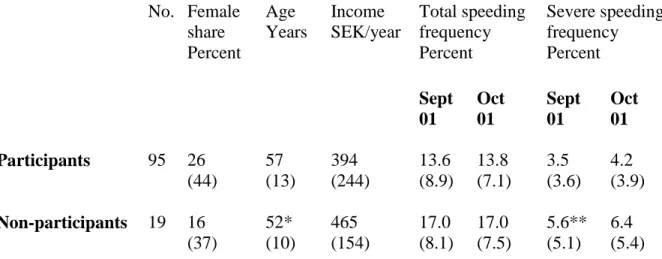
Table 2. Average characteristics of participants (groups A-F) and non-participants (group
G): Sex, age, annual income, and speeding frequency (Total and Severe speeding time, respectively, as percent of total driving time) of operated cars. Standard errors within parentheses. No. Female share Percent Age Years Income SEK/year Total speeding frequency Percent Severe speeding frequency Percent Sept 01 Oct 01 Sept 01 Oct 01 Participants 95 26 (44) 57 (13) 394 (244) 13.6 (8.9) 13.8 (7.1) 3.5 (3.6) 4.2 (3.9) Non-participants 19 16 (37) 52* (10) 465 (154) 17.0 (8.1) 17.0 (7.5) 5.6** (5.1) 6.4 (5.4) * Difference between participants and non-participants is significant at the 10% level ** Difference between participants and non-participants is significant at the 5% level
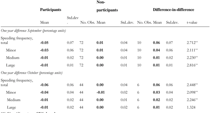
Table 3. 12-months differences in average speeding frequency, percentage units.
Participants
Non-
participants Difference-in-difference
Mean Std.dev. No. Obs. Mean Std..dev. No. Obs. Mean Std.dev. t-value
One-year difference September (percentage units)
Speeding frequency,
total -0.05 0.07 72 0.01 0.04 10 0.06 0.07 2.712**
Minor -0.03 0.06 72 0.01 0.04 10 0.04 0.06 2.111**
Medium -0.01 0.02 72 0.00 0.01 10 0.01 0.02 2.230**
Large -0.01 0.01 72 0.00 0.01 10 0.01 0.01 2.816**
One-year difference October (percentage units)
Speeding frequency, total -0.06 0.06 44 0.00 0.04 6 0.06 0.06 2.448** Minor -0.04 0.04 44 -0.01 0.02 6 0.03 0.04 2.098** Medium -0.01 0.02 44 0.00 0.01 6 0.02 0.02 2.246** Large -0.01 0.02 44 0.00 0.02 6 0.01 0.02 1.324 **) Significant on 95% level.
Table 4. Average socio-economic characteristics (sex, age, income) of non-participants
(group G) , treatment groups (A-F), and aggregates of treatment groups
Group G C E D F A B ACE BDF EF CD AB CDEF
Bonus 0 H H L L H L H L
Pernalty 0 L H L H 0 0 H L 0 H+L
Sex 0,16 0,44 0,25 0,13 0,31 0,25 0,3 0,31 0,25 0,28 0,29 0,28 0,28
Age 52 57,7 52,4 63,9 52 58,6 59,7 56,2 58,5 52,2 60,8 59,2 56,5
Table 5. OLS estimation results for one-year differences of Severe speeding in the
September and October samples, respectively. Base (general) and reduced (specific) models. Standard errors within parentheses.
Variable September 01-02 October 01-02
Base Reduced Base Reduced
Constant -0.025 (0.045) 0.015 (0.014) -0.053 (0.070) -0.001 (0.006) Participation 0.025** (0.011) 0.026*** (0.009) 0.009 (0.018) Penalty 0.004 (0.008) 0.018 (0.012) 0.021** (0.008) High penalty -0.002 (0.008) 0.005 (0.013) High Bonus -0.001 (0.007) 0.004 0.010 Sex 0.0003 (0.0075) 0.032*** (0.011) 0.062*** (0.013) Age 0.001 (0.002) 0.002 (0.003) Age-squared -0.000015 (0.000015) -0.00002 (0.00002) Income 0.000005 (0.000012) -0.000037** (0.000015) Income*Sex -0.000061*** (0.000018) R-squared 13.8 11.8 43.0 47.2 Numb. Obs. 79 81 47 47
Figure 1. Speed profile of car #58 on roads with speed limit 50 km/h September 2001
(without penalty charges) and September 2002 (with penalty charges)
0 0.02 0.04 0.06 0.08 0.1 0.12 0.14 0.16 0.18 0.2 2.5 7.5 12.5 17.5 22.5 27.5 32.5 37.5 42.5 47.5 52.5 57.5 62.5 67.5 72.5 77.5 Km/h Fr eq ue nc e Sept 01 Sept 02 Type I Type II Type III
Figure 3Average speeding frequency of participants (Yes) and non-participants (No)
autumn months of 2001 and 2002. (YesNov represent drivers that accepted to continue the economic experiment for a third month).
0.00 0.02 0.04 0.06 0.08 0.10 0.12 0.14 0.16 0.18
Sept 2001 Oct 2001 Nov 2001 Sept 2002 Oct 2002 Nov 2002
Yes No YesNov
Figure 4. Effects on speeding frequency of penalties. One-year differences per month. September -70,00% -60,00% -50,00% -40,00% -30,00% -20,00% -10,00% 0,00% 10,00% 20,00%
Minor Medium Major Total
G A+B C+D E+F October -80% -70% -60% -50% -40% -30% -20% -10% 0% 10% 20%
Minor Medium Major Total
G A+B C+D E+F
Figure 5. Effects of High Bonus (Groups B+D) vs. Low Bonus (Groups A+C). One-year
differences per month. September -80% -70% -60% -50% -40% -30% -20% -10% 0% 10% 20% 30%
Minor Medium Major Total
G A+C B+D October -80% -70% -60% -50% -40% -30% -20% -10% 0% 10% 20%
Minor Medium Major Total
G A+C B+D
Appendix.
Table A1. OLS estimation results of Severe speeding frequency in September and
October 2001, respectively. Standard errors within parentheses. Variable September 01 October 01
Constant 0.009 (0.061) -0.022 (0.082) Participant -0.016 (0.010) -0.015 (0.014) Sex 0.010 (0.010) 0.012 (0.012) Age 0.002 (0.002) 0.003 (0.003) Age-squared -0.00003 (0.00002) -0.00004 (0.00003) Income 0.000008 (0.000016) 0.000018 (0.0000019) R-squared 12.2 15.2 Numb. Obs. 98 70
Table A2. Average socio-economic characteristics (sex, age, income) of non-participants
(group G) , treatment groups (A-F), and aggregates of treatment groups
Group G C E D F A B ACE BDF EF CD AB CDEF
Bonus 0 H H L L H L H L
Pernalty 0 L H L H 0 0 H L 0 H+L
Sex 0,16 0,44 0,25 0,13 0,31 0,25 0,3 0,31 0,25 0,28 0,29 0,28 0,28
Age 52 57,7 52,4 63,9 52 58,6 59,7 56,2 58,5 52,2 60,8 59,2 56,5
Table A3. Summary statistics September sample.
Variable Obs. Mean Std. Dev. Min Max
Sex 81 0.235 0.426 0 1 Age 81 57.6 13.0 25 81 Age-squared 81 3483 1444 625 6561 Income 79 427 255 67 1929 Participant 81 0.877 0.331 0 1 Penalty 81 0.593 0.494 0 1 High penalty 81 0.296 0.459 0 1 High bonus 81 0.444 0.500 0 1 DiffSevere 81 0.0167 0.0268 -0.0289 0.1342
Table A4. Summary statistics October sample.
Variable Obs. Mean Std. Dev. Min Max
Sex 48 0.313 0.468 0 1 Age 48 58.9 13.4 29 81 Age-squared 48 3640 1537 841 6561 Income 47 451 297 167 1929 Participant 48 0.875 0.334 0 1 Penalty 48 0.583 0.498 0 1 High penalty 48 0.229 0.425 0 1 High bonus 48 0.438 0.501 0 1 DiffSevere 48 0.0190 0.0351 -0.0840 0.1035